WEALTH, DISPOSABLE INCOME AND CONSUMPTION - Economics

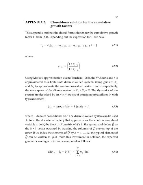
APPENDIX 2: Closed-form solution for the cumulative
growth factors
This appendix outlines the closed-form solution for the cumulative growth
factor Γ from (2.4). Expanding out the expression for Γ we have
where
Γt = Et[ qt + 1+
qt + 1qt
+ 2 + qt + 1qt
+ 2qt
+ 3+
…]
qt + i
⎛1 + xt + i⎞
= ⎜------------------- ⎟
⎝1+ r ⎠ t + i
57
(A1)
(A2)
Using Markov approximation due to Tauchen (1986), the VAR for x and r is
approximated as a finite-state discrete-valued system. Using grids of Nx and Nr to approximate the continuous-valued series x and r respectively,
the state space of the dicrete system is Nx × Nr ≡ N.
The dynamics of the
system are described by an N × N matrix of transition probabilities Φ with
typical element
φk, l=
prob[state = k state = l]
(A3)
where denotes “conditional on.” The discrete-valued system can be used
to form the discrete variable qˆ that approximates the continuous-valued
variable q. Let Q be the Nx × Nr matrix of qˆ’s in the system and define Q as
the N × 1 vector obtained by stacking the columns of Q one on top of the
other. If we index the elements of Q by k = 1, …, N,
the typical element of
Q can be written as qˆ( k)
. With this investment in notation, the expected
geometric averages of qˆ can be computed as follows:
E[qˆ t 1
+ qˆt= qˆ( k)]
=
φk, lqˆ()
l
N
∑
l= 1
(A4)