Compact beamforming in medical ultrasound scanners
Compact beamforming in medical ultrasound scanners
Compact beamforming in medical ultrasound scanners

Create successful ePaper yourself
Turn your PDF publications into a flip-book with our unique Google optimized e-Paper software.
<strong>Compact</strong> <strong>beamform<strong>in</strong>g</strong> <strong>in</strong> <strong>medical</strong><br />
<strong>ultrasound</strong> <strong>scanners</strong><br />
Borislav Gueorguiev Tomov<br />
January 31, 2003<br />
Ørsted•DTU<br />
Technical University of Denmark
SUBMITTED IN PARTIAL FULFILLMENT OF THE<br />
REQUIREMENTS FOR THE DEGREE OF<br />
DOCTOR OF PHILOSOPHY<br />
AT<br />
THE TECHNICAL UNIVERSITY OF DENMARK<br />
JANUARY 2003<br />
Signature of Author<br />
THE AUTHOR RESERVES OTHER PUBLICATION RIGHTS, AND NEITHER THE THE-<br />
SIS NOR EXTENSIVE EXTRACTS FROM IT MAY BE PRINTED OR OTHERWISE REPRO-<br />
DUCED WITHOUT THE AUTHOR’S WRITTEN PERMISSION.<br />
THE AUTHOR ATTESTS THAT PERMISSION HAS BEEN OBTAINED FOR THE USE OF<br />
ANY COPYRIGHTED MATERIAL APPEARING IN THIS THESIS (OTHER THAN BRIEF EX-<br />
CERPTS REQUIRING ONLY PROPER ACKNOWLEDGEMENT IN SCHOLARLY WRITING)<br />
AND THAT ALL SUCH USE IS CLEARLY ACKNOWLEDGED.<br />
c○ Copyright by Borislav G. Tomov 2004<br />
All Rights Reserved
To my sister Tanya
Contents<br />
Contents i<br />
Abstract iii<br />
Preface v<br />
Acknowledgments vii<br />
List of Figures xiii<br />
List of Tables xiv<br />
1 Introduction 1<br />
1.1 Ultrasound imag<strong>in</strong>g pr<strong>in</strong>ciple . . . . . . . . . . . . . . . . . . . . . . . . . . 2<br />
1.2 Medical <strong>ultrasound</strong> systems evolution . . . . . . . . . . . . . . . . . . . . . . 2<br />
1.3 Blood velocity estimation . . . . . . . . . . . . . . . . . . . . . . . . . . . . 4<br />
1.3.1 Sonogram / Spectral Doppler . . . . . . . . . . . . . . . . . . . . . . 5<br />
1.3.2 Color flow map . . . . . . . . . . . . . . . . . . . . . . . . . . . . . 6<br />
1.4 Comparison with CT and MR imag<strong>in</strong>g . . . . . . . . . . . . . . . . . . . . . 8<br />
1.4.1 Computed tomography . . . . . . . . . . . . . . . . . . . . . . . . . 8<br />
1.4.2 Magnetic resonance imag<strong>in</strong>g . . . . . . . . . . . . . . . . . . . . . . 8<br />
1.4.3 Ultrasound imag<strong>in</strong>g . . . . . . . . . . . . . . . . . . . . . . . . . . . 9<br />
2 Ultrasound acoustics 10<br />
2.1 Wave equation . . . . . . . . . . . . . . . . . . . . . . . . . . . . . . . . . . 10<br />
2.2 Solutions to the wave equation . . . . . . . . . . . . . . . . . . . . . . . . . . 10<br />
2.2.1 Plane wave . . . . . . . . . . . . . . . . . . . . . . . . . . . . . . . 10<br />
2.2.2 Spherical wave . . . . . . . . . . . . . . . . . . . . . . . . . . . . . 11<br />
2.3 Wavenumber-frequency space (k-space) . . . . . . . . . . . . . . . . . . . . . 12<br />
i
2.4 Propagation <strong>in</strong> tissue . . . . . . . . . . . . . . . . . . . . . . . . . . . . . . . 12<br />
2.4.1 Reflection . . . . . . . . . . . . . . . . . . . . . . . . . . . . . . . . 13<br />
2.4.2 Scatter<strong>in</strong>g . . . . . . . . . . . . . . . . . . . . . . . . . . . . . . . . 13<br />
2.4.3 Attenuation . . . . . . . . . . . . . . . . . . . . . . . . . . . . . . . 14<br />
3 Beamformation 15<br />
3.1 Transducer properties . . . . . . . . . . . . . . . . . . . . . . . . . . . . . . 15<br />
3.1.1 Directivity properties of f<strong>in</strong>ite cont<strong>in</strong>uous apertures . . . . . . . . . . 15<br />
3.1.2 Angular resolution concept . . . . . . . . . . . . . . . . . . . . . . . 16<br />
3.1.3 Directivity properties of arrays . . . . . . . . . . . . . . . . . . . . . 17<br />
3.1.4 Directivity properties of arrays of f<strong>in</strong>ite cont<strong>in</strong>uous sensors . . . . . . 19<br />
3.1.5 Phased array angular resolution dependence on the <strong>in</strong>cidence angle . . 20<br />
3.2 Focus<strong>in</strong>g . . . . . . . . . . . . . . . . . . . . . . . . . . . . . . . . . . . . . 20<br />
3.2.1 Focus<strong>in</strong>g geometry . . . . . . . . . . . . . . . . . . . . . . . . . . . 22<br />
3.2.2 Influence of the speed of sound . . . . . . . . . . . . . . . . . . . . . 23<br />
3.2.3 Influence of the delay precision . . . . . . . . . . . . . . . . . . . . . 23<br />
3.3 Beamform<strong>in</strong>g . . . . . . . . . . . . . . . . . . . . . . . . . . . . . . . . . . . 24<br />
3.3.1 Transducer element directivity implications . . . . . . . . . . . . . . 26<br />
3.4 Beamform<strong>in</strong>g techniques . . . . . . . . . . . . . . . . . . . . . . . . . . . . . 27<br />
3.5 Comparison between focus<strong>in</strong>g techniques . . . . . . . . . . . . . . . . . . . . 29<br />
3.6 Conclusion . . . . . . . . . . . . . . . . . . . . . . . . . . . . . . . . . . . . 30<br />
4 Compression of the the focus<strong>in</strong>g data 35<br />
4.1 Memory requirements <strong>in</strong> <strong>ultrasound</strong> <strong>beamform<strong>in</strong>g</strong> . . . . . . . . . . . . . . . 36<br />
4.2 Delay calculation . . . . . . . . . . . . . . . . . . . . . . . . . . . . . . . . . 37<br />
4.3 Delta encod<strong>in</strong>g . . . . . . . . . . . . . . . . . . . . . . . . . . . . . . . . . . 39<br />
4.4 Piecewise-l<strong>in</strong>ear approximation . . . . . . . . . . . . . . . . . . . . . . . . . 40<br />
4.5 General parametric approach . . . . . . . . . . . . . . . . . . . . . . . . . . . 42<br />
4.5.1 Transformation to clock periods (clock cycles) . . . . . . . . . . . . . 42<br />
4.5.2 Delay values generation . . . . . . . . . . . . . . . . . . . . . . . . . 42<br />
4.6 LUCS delay generator . . . . . . . . . . . . . . . . . . . . . . . . . . . . . . 43<br />
4.7 Comparison between approximation schemes . . . . . . . . . . . . . . . . . . 45<br />
4.8 Discussion . . . . . . . . . . . . . . . . . . . . . . . . . . . . . . . . . . . . 46<br />
5 Delta-Sigma modulation A/D conversion 47<br />
5.1 Pr<strong>in</strong>ciple of operation . . . . . . . . . . . . . . . . . . . . . . . . . . . . . . 48<br />
5.1.1 Signal-to-quantization-noise ratio (SQNR) of a multi-bit Nyquist-rate<br />
data converter . . . . . . . . . . . . . . . . . . . . . . . . . . . . . . 48<br />
5.1.2 SQNR of oversampl<strong>in</strong>g converters . . . . . . . . . . . . . . . . . . . 50<br />
5.2 Sample reconstruction . . . . . . . . . . . . . . . . . . . . . . . . . . . . . . 57<br />
5.3 Higher-order noise shap<strong>in</strong>g and band-pass modulators . . . . . . . . . . . . . 57<br />
ii
6 DSM beamformer 58<br />
6.1 Previous approaches for utiliz<strong>in</strong>g DSM <strong>in</strong> beamformers . . . . . . . . . . . . 58<br />
6.1.1 Modified modulator architecture for compensation of sample drop or<br />
<strong>in</strong>sertion . . . . . . . . . . . . . . . . . . . . . . . . . . . . . . . . . 59<br />
6.1.2 Use of non-uniform sampl<strong>in</strong>g clock . . . . . . . . . . . . . . . . . . 61<br />
6.2 New architecture for an oversampled beamformer . . . . . . . . . . . . . . . 62<br />
6.2.1 Sparse sample process<strong>in</strong>g concept . . . . . . . . . . . . . . . . . . . 62<br />
6.2.2 Signal process<strong>in</strong>g . . . . . . . . . . . . . . . . . . . . . . . . . . . . 64<br />
6.2.3 Choice of reconstruction filter . . . . . . . . . . . . . . . . . . . . . 64<br />
6.2.4 Calculation of the necessary oversampl<strong>in</strong>g ratio . . . . . . . . . . . . 65<br />
6.2.5 Simulation results . . . . . . . . . . . . . . . . . . . . . . . . . . . . 67<br />
6.2.6 Phantom data process<strong>in</strong>g results . . . . . . . . . . . . . . . . . . . . 68<br />
6.3 Discussion . . . . . . . . . . . . . . . . . . . . . . . . . . . . . . . . . . . . 68<br />
7 Implementation 74<br />
7.1 Sample buffer . . . . . . . . . . . . . . . . . . . . . . . . . . . . . . . . . . . 75<br />
7.2 Delay generation logic . . . . . . . . . . . . . . . . . . . . . . . . . . . . . . 76<br />
7.3 Apodization . . . . . . . . . . . . . . . . . . . . . . . . . . . . . . . . . . . 77<br />
7.4 Summ<strong>in</strong>g block . . . . . . . . . . . . . . . . . . . . . . . . . . . . . . . . . . 78<br />
7.5 Filters for <strong>in</strong>-phase and quadrature component . . . . . . . . . . . . . . . . . 78<br />
7.6 Interface . . . . . . . . . . . . . . . . . . . . . . . . . . . . . . . . . . . . . 79<br />
7.7 Synthesis results for a 32-channel beamformer . . . . . . . . . . . . . . . . . 80<br />
8 Conclusion 81<br />
A A new architecture for a s<strong>in</strong>gle-chip multi-channel beamformer based on a standard<br />
FPGA 82<br />
1 Introduction . . . . . . . . . . . . . . . . . . . . . . . . . . . . . . . . . . . 83<br />
2 Pr<strong>in</strong>ciples beh<strong>in</strong>d the suggested beamformer architecture . . . . . . . . . . . . 84<br />
2.1 Rationale for the sparse sample process<strong>in</strong>g . . . . . . . . . . . . . . . 84<br />
2.2 Usage of the Delta-Sigma modulator <strong>in</strong> the beamformer . . . . . . . . 84<br />
2.3 Delay generation . . . . . . . . . . . . . . . . . . . . . . . . . . . . 85<br />
3 Beamformer architecture . . . . . . . . . . . . . . . . . . . . . . . . . . . . . 87<br />
4 Implementation tradeoffs and choices . . . . . . . . . . . . . . . . . . . . . . 87<br />
5 Phantom data process<strong>in</strong>g results . . . . . . . . . . . . . . . . . . . . . . . . . 89<br />
6 Conclusion . . . . . . . . . . . . . . . . . . . . . . . . . . . . . . . . . . . . 89<br />
B Delay generation methods with reduced memory requirements 91<br />
1 Memory requirements <strong>in</strong> <strong>ultrasound</strong> <strong>beamform<strong>in</strong>g</strong> . . . . . . . . . . . . . . . 92<br />
2 Index generation geometry . . . . . . . . . . . . . . . . . . . . . . . . . . . . 94<br />
3 General parametric approach . . . . . . . . . . . . . . . . . . . . . . . . . . . 95<br />
3.1 Transformation to clock periods (clock cycles) . . . . . . . . . . . . . 96<br />
iii
3.2 Influence of the directivity properties of the transducer elements . . . 96<br />
3.3 Delay generation algorithm . . . . . . . . . . . . . . . . . . . . . . . 98<br />
4 LUCS delay generator . . . . . . . . . . . . . . . . . . . . . . . . . . . . . . 98<br />
5 Piecewise-l<strong>in</strong>ear approximation . . . . . . . . . . . . . . . . . . . . . . . . . 100<br />
6 Comparison between <strong>in</strong>dex generation techniques . . . . . . . . . . . . . . . 101<br />
7 Discussion . . . . . . . . . . . . . . . . . . . . . . . . . . . . . . . . . . . . 102<br />
8 Conclusion . . . . . . . . . . . . . . . . . . . . . . . . . . . . . . . . . . . . 103<br />
C <strong>Compact</strong> FPGA-based beamformer us<strong>in</strong>g oversampled 1-bit AD converters 104<br />
1 Introduction . . . . . . . . . . . . . . . . . . . . . . . . . . . . . . . . . . . 104<br />
2 Traditional beamformer architecture . . . . . . . . . . . . . . . . . . . . . . . 106<br />
3 New beamformer features . . . . . . . . . . . . . . . . . . . . . . . . . . . . 107<br />
3.1 Sparse sample process<strong>in</strong>g . . . . . . . . . . . . . . . . . . . . . . . . 107<br />
3.2 Beamform<strong>in</strong>g with oversampled signals . . . . . . . . . . . . . . . . 109<br />
3.3 Reconstruction filters . . . . . . . . . . . . . . . . . . . . . . . . . . 111<br />
4 Image quality . . . . . . . . . . . . . . . . . . . . . . . . . . . . . . . . . . . 111<br />
4.1 Calculat<strong>in</strong>g the necessary sampl<strong>in</strong>g frequency . . . . . . . . . . . . . 112<br />
4.2 Simulation results . . . . . . . . . . . . . . . . . . . . . . . . . . . . 113<br />
4.3 Phantom image . . . . . . . . . . . . . . . . . . . . . . . . . . . . . 115<br />
5 Implementation . . . . . . . . . . . . . . . . . . . . . . . . . . . . . . . . . . 115<br />
5.1 Implementation results . . . . . . . . . . . . . . . . . . . . . . . . . 117<br />
6 Discussion . . . . . . . . . . . . . . . . . . . . . . . . . . . . . . . . . . . . 117<br />
7 Conclusion . . . . . . . . . . . . . . . . . . . . . . . . . . . . . . . . . . . . 117<br />
Bibliography 127<br />
iv
Abstract<br />
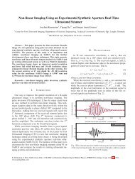
This Ph.D. project was carried out at the Center for Fast Ultrasound Imag<strong>in</strong>g, Technical University<br />
of Denmark, under the supervision of Prof. Jørgen Arendt Jensen, Assoc. Prof. Jens<br />
Sparsø and Prof. Erik Bruun. The goal was to <strong>in</strong>vestigate methods for efficient <strong>beamform<strong>in</strong>g</strong>,<br />
which make it possible to fit a large number of channels on a s<strong>in</strong>gle <strong>in</strong>tegrated circuit. The use<br />
of oversampled analog-to-digital (A/D) converters with the correspond<strong>in</strong>g <strong>beamform<strong>in</strong>g</strong> was<br />
identified as a particularly promis<strong>in</strong>g approach, s<strong>in</strong>ce it provides both <strong>in</strong>expensive and compact<br />
A/D conversion and allows for much more compact implementation of the beamformer<br />
compared to the case where conventional A/D conversion is used.<br />
The compact and economic <strong>beamform<strong>in</strong>g</strong> is a key aspect <strong>in</strong> the progress of <strong>medical</strong> <strong>ultrasound</strong><br />
imag<strong>in</strong>g. Currently, 64 or 128 channels are widely used <strong>in</strong> <strong>scanners</strong>, top-of-the-range <strong>scanners</strong><br />
have 256 channels, and even more channels are necessary for 3-dimensional (3D) diagnostic<br />
imag<strong>in</strong>g. On the other hand, there is a demand for <strong>in</strong>expensive portable devices for use outside<br />
hospitals, <strong>in</strong> field conditions, where power consumption and compactness are important factors.<br />
The thesis starts with an <strong>in</strong>troduction <strong>in</strong>to <strong>medical</strong> <strong>ultrasound</strong>, its basic pr<strong>in</strong>ciples, system evolution<br />
and its place among <strong>medical</strong> imag<strong>in</strong>g techniques. Then, <strong>ultrasound</strong> acoustics is <strong>in</strong>troduced,<br />
as a necessary base for understand<strong>in</strong>g the concepts of acoustic focus<strong>in</strong>g and <strong>beamform<strong>in</strong>g</strong>,<br />
which follow. The necessary focus<strong>in</strong>g <strong>in</strong>formation for high-quality imag<strong>in</strong>g is large, and<br />
compress<strong>in</strong>g it leads to better compactness of the beamformers. The exist<strong>in</strong>g methods for compress<strong>in</strong>g<br />
and recursive generation of focus<strong>in</strong>g data, along with orig<strong>in</strong>al work <strong>in</strong> the area, are<br />
presented <strong>in</strong> Chapter 4.<br />
The pr<strong>in</strong>ciples and the performance limitations of the oversampled delta-sigma converters are<br />
given <strong>in</strong> Chapter 5, followed by an overview of the present architectures of oversampled beamformers.<br />
Then, a new architecture is <strong>in</strong>troduced, which has the potential of achiev<strong>in</strong>g the<br />
highest image quality that an oversampl<strong>in</strong>g beamformer can provide. That architecture has<br />
been implemented us<strong>in</strong>g VHDL, and estimates for its performance have been obta<strong>in</strong>ed. The results<br />
<strong>in</strong>dicate that a 32-channel beamformer reaches the target operation frequency of 140MHz,<br />
thereby provid<strong>in</strong>g diagnostic image with dynamic range of 60 dB for an excitation central fre-<br />
iii
Contents<br />
quency of 3MHz. That image quality is comparable to that of the very good <strong>scanners</strong> currently<br />
on the market. The performance results have been achieved with the use of a simple oversampled<br />
converter of second order. The use of a higher order oversampled converter will allow<br />
higher pulse frequency to be used while the high dynamic range <strong>in</strong> the end image is preserved.<br />
The logic resource utilization of a Xil<strong>in</strong>x FPGA device XCV2000E-7 is less than 45 % when a<br />
32-channel beamformer is implemented. The maximum number of channels that can fit <strong>in</strong> that<br />
FPGA device is 57, due to the fact that too many of the available gates take part <strong>in</strong> the rout<strong>in</strong>g<br />
when the channel number is <strong>in</strong>creased.<br />
iv
Preface<br />
The <strong>in</strong>itial name of this Ph.D. project was ”Integrated circuits <strong>in</strong> <strong>medical</strong> <strong>ultrasound</strong>”, with<br />
the goal of <strong>in</strong>vestigat<strong>in</strong>g the <strong>in</strong>tegrated circuits necessary for the implementation of advanced<br />
<strong>medical</strong> <strong>ultrasound</strong> imag<strong>in</strong>g techniques. By the time of the submission of the study plan, a<br />
more specific goal was chosen: to <strong>in</strong>vestigate methods for efficient <strong>beamform<strong>in</strong>g</strong>, which make<br />
it possible to fit a large number of channels on a s<strong>in</strong>gle <strong>in</strong>tegrated circuit. The use of oversampled<br />
analog-to-digital (A/D) converters was identified as an attractive concept, lead<strong>in</strong>g to the<br />
development of very compact beamformers.<br />
Dur<strong>in</strong>g the Ph.D. study, the follow<strong>in</strong>g papers were published:<br />
• B. G. Tomov and J. A. Jensen. A new architecture for a s<strong>in</strong>gle-chip multi-channel beamformer<br />
based on a standard FPGA. In Proceed<strong>in</strong>gs of the IEEE Ultrasonics Symposium,<br />
volume 2, pages 1529-1533, 2001.<br />
• B. G. Tomov and J. A. Jensen. Delay generations with reduced memory requirements, <strong>in</strong><br />
Proceed<strong>in</strong>gs of SPIE Vol. 5035 Medical Imag<strong>in</strong>g 2003:Ultrasonic Imag<strong>in</strong>g and Signal<br />
Process<strong>in</strong>g, edited by William F. Walker, Michael F. Insana, (SPIE, Bell<strong>in</strong>gham, WA,<br />
2003) pages 491-500.<br />
• B. G. Tomov and J. A. Jensen. <strong>Compact</strong> FPGA-based beamformer us<strong>in</strong>g oversampled 1bit<br />
AD converters”, In IEEE Transactions on Ultrasonics, Ferroelectrics, and Frequency<br />
Control”, Submitted for publication, 2003.<br />
Their content is given <strong>in</strong> the appendices.<br />
The <strong>in</strong>centive for the present work was the aspiration for compact and <strong>in</strong>expensive <strong>scanners</strong>,<br />
which I and my adviser Jørgen Arendt Jensen shared. Three years ago, <strong>ultrasound</strong> <strong>scanners</strong><br />
were expensive and bulky mach<strong>in</strong>es, and portable <strong>scanners</strong> were not on the market yet. Prof.<br />
Jensen had the vision of mak<strong>in</strong>g the <strong>ultrasound</strong> diagnostic devices as common as the stethoscopes.<br />
Although one should have certa<strong>in</strong> basic tra<strong>in</strong><strong>in</strong>g <strong>in</strong> order to be able to use such a<br />
v
Contents<br />
device and make a correct diagnosis, the presence of <strong>in</strong>expensive <strong>scanners</strong> on the market will<br />
be beneficial for the patients <strong>in</strong> the long run.<br />
Oversampled data converters - both A/D and D/A, have proven themselves <strong>in</strong> audio and<br />
telecommunication. Their use, along with other technological improvements, has facilitated the<br />
wide spread of high-quality data conversion, lead<strong>in</strong>g to affordable Hi-Fi audio and <strong>in</strong>expensive<br />
communications. What makes the oversampled converters so wide spread is their suitability<br />
for CMOS implementation. They can be implemented along the digital logic on a chip, thus<br />
enabl<strong>in</strong>g a s<strong>in</strong>gle-chip devices to <strong>in</strong>terface the analog environment. It can be expected that <strong>in</strong> a<br />
few years multiple delta-sigma modulators on a s<strong>in</strong>gle chip will be mass-produced and will be<br />
used <strong>in</strong> <strong>ultrasound</strong> <strong>scanners</strong>, br<strong>in</strong>g<strong>in</strong>g simplified connections and beamformation.<br />
The limit<strong>in</strong>g factor for the use of oversampled converters is the necessary high oversampl<strong>in</strong>g<br />
ratio, which, together with the complexity of the modulators, determ<strong>in</strong>es the quality of the<br />
conversion. This is the reason why there are not many examples of oversampled converters for<br />
video signals and higher frequency signals.<br />
This thesis describes my research <strong>in</strong> oversampled beamformers and other means for achiev<strong>in</strong>g<br />
compact beamformation. I hope that it is a useful read<strong>in</strong>g and it is a good base for further<br />
research <strong>in</strong> that area.<br />
vi
Acknowledgments<br />
My adviser, prof. Jørgen Arendt Jensen, is the person who made this work possible. I am<br />
deeply grateful to him for his guidance, patience and understand<strong>in</strong>g. His suggestion that I get<br />
acqua<strong>in</strong>ted with oversampled converters led to the choice of the present research area, which<br />
has been <strong>in</strong>terest<strong>in</strong>g and excit<strong>in</strong>g. His idea for sparse sample process<strong>in</strong>g made it possible to<br />
use FIR filters for sample reconstruction, thus achiev<strong>in</strong>g high image quality. On numerous<br />
occasions, I had the privilege to learn from his example the proper scientific research practices.<br />
I highly appreciate the opportunity to work with him.<br />
I am grateful to my advisers Jens Sparsø and Erik Bruun for their care and attention through<br />
my study.<br />
I would like to thank all my colleagues at the Center for Fast Ultrasound Imag<strong>in</strong>g for creat<strong>in</strong>g<br />
a helpful and positive environment. In particular I would like to thank:<br />
• my colleague from the Technical University of Sofia and the Radar school <strong>in</strong> the army,<br />
Svetoslav Ivanov Nikolov, for present<strong>in</strong>g to me the opportunity to study as a Ph.D. student<br />
at CFU and encourag<strong>in</strong>g me to apply for the position. Dur<strong>in</strong>g these years, he helped<br />
me with technical expertise (L<strong>in</strong>ux, Matlab and programm<strong>in</strong>g) and <strong>in</strong>spir<strong>in</strong>g discussions<br />
on <strong>ultrasound</strong> imag<strong>in</strong>g. He also k<strong>in</strong>dly donated the LaTeX style for the present thesis.<br />
He has been a very good friend.<br />
• Peter Munk, with whom we worked on the experimental sampl<strong>in</strong>g system RASMUS.<br />
Apart form his k<strong>in</strong>d and helpful attitude dur<strong>in</strong>g his stay at the Center, it was an enjoyable<br />
experience for me to work <strong>in</strong> a team with a person as competent and as dedicated as him.<br />
• Malene Schlaikjer, for help<strong>in</strong>g me with many practical aspects of my study and residence<br />
<strong>in</strong> the well organized country of Denmark.<br />
• Thanassis Misaridis, for be<strong>in</strong>g a friendly and cheer<strong>in</strong>g co-worker.<br />
• Kim Løkke Gammelmark, for be<strong>in</strong>g a great officemate and a helpful colleague.<br />
vii
Contents<br />
• Henrik Møller Pedersen, for be<strong>in</strong>g very helpful and co-operative dur<strong>in</strong>g my first months<br />
at the Center for Fast Ultrasound Imag<strong>in</strong>g.<br />
• Paul David Fox, Jens Vilhjelm and Kaj- ˚Age Henneberg, for their cooperation on various<br />
work-related occasions and their friendly attitude.<br />
I would also like to thank our system adm<strong>in</strong>istrator Henrik Laursen and our hardware specialist<br />
Benny Johansen, for be<strong>in</strong>g very helpful and quick with resolv<strong>in</strong>g software and hardware issues.<br />
Dur<strong>in</strong>g the test<strong>in</strong>g and the debugg<strong>in</strong>g of the <strong>ultrasound</strong> sampl<strong>in</strong>g system RASMUS I had the<br />
opportunity to work with dedicated and <strong>in</strong>spir<strong>in</strong>g people like Mart<strong>in</strong> Hansen, Ole Holm, Henrik<br />
Bendsen, Lars Joost Jensen and Kim Gormsen from I/O Consult<strong>in</strong>g A/S, and I would like to<br />
thank them for that experience.<br />
I would like to thank Villy Brænder from B-K Medical A/S for his support and cooperation <strong>in</strong><br />
the recent months.<br />
Last, but not least, I would like to thank my wife, Rayna Georgieva, for her lov<strong>in</strong>g and support<br />
through these years.<br />
This work was made possible thanks to f<strong>in</strong>ancial support from the Danish Science Foundation<br />
(grants 9700883 and 9700563), from B-K Medical A/S, Herlev, Denmark, from the Thomas B.<br />
Thrige Center for Micro<strong>in</strong>struments, and from the Danish Research Academy.<br />
viii
List of Figures<br />
1.1 Illustration of the pr<strong>in</strong>ciple of <strong>ultrasound</strong> imag<strong>in</strong>g. . . . . . . . . . . . . . . . . 1<br />
1.2 A-mode system architecture. . . . . . . . . . . . . . . . . . . . . . . . . . . . 3<br />
1.3 M-mode system architecture. . . . . . . . . . . . . . . . . . . . . . . . . . . . 3<br />
1.4 Real-time B-mode system architecture. . . . . . . . . . . . . . . . . . . . . . . 4<br />
1.5 Multi-element transducers: L<strong>in</strong>ear array (left) and phased array(right). The<br />
beam positions are shown with gray dashed l<strong>in</strong>e, and the spatial extent of one<br />
beam is shown with black l<strong>in</strong>e. . . . . . . . . . . . . . . . . . . . . . . . . . . 5<br />
1.6 Triplex mode image, show<strong>in</strong>g B-mode image, spectral Doppler (bottom graphics)<br />
and color flow map of the carotid artery (image courtesy of B-K Medical<br />
A/S). . . . . . . . . . . . . . . . . . . . . . . . . . . . . . . . . . . . . . . . . 6<br />
1.7 Analog demodulation module. . . . . . . . . . . . . . . . . . . . . . . . . . . 7<br />
2.1 Transmission and reflection of a plane wave propagat<strong>in</strong>g obliquely to medium<br />
border. . . . . . . . . . . . . . . . . . . . . . . . . . . . . . . . . . . . . . . . 14<br />
3.1 Cont<strong>in</strong>uous l<strong>in</strong>ear aperture and its response to a propagat<strong>in</strong>g cont<strong>in</strong>uous plane<br />
wave (aperture smooth<strong>in</strong>g function). . . . . . . . . . . . . . . . . . . . . . . . 16<br />
3.2 Directivity pattern of a cont<strong>in</strong>uous l<strong>in</strong>ear aperture. . . . . . . . . . . . . . . . . 17<br />
3.3 Aperture smooth<strong>in</strong>g function of an array of omnidirectional sensors. . . . . . . 18<br />
3.4 Grat<strong>in</strong>g lobes generation. Isophase surfaces spaced at 2π are drawn <strong>in</strong> gray. . . 18<br />
ix
List of Figures<br />
3.5 Directivity pattern of a 3λ-spaced 12-element array with no gaps between elements<br />
and with 15 % gaps. The array response is shown <strong>in</strong> gray and the sensor<br />
element response is shown <strong>in</strong> black <strong>in</strong> the upper plots. The lower plots show<br />
the result<strong>in</strong>g response. . . . . . . . . . . . . . . . . . . . . . . . . . . . . . . 19<br />
3.6 Angular resolution (angle of the first zero <strong>in</strong> the directivity pattern) of an array<br />
with size 32λ, given as a function of angle of <strong>in</strong>cidence of the <strong>in</strong>com<strong>in</strong>g wave. . 21<br />
3.7 Illustration of near field (<strong>ultrasound</strong>) and far field (radar). . . . . . . . . . . . . 21<br />
3.8 Focus<strong>in</strong>g geometry . . . . . . . . . . . . . . . . . . . . . . . . . . . . . . . . 22<br />
3.9 Analog signal transformations <strong>in</strong> an <strong>ultrasound</strong> imag<strong>in</strong>g system. . . . . . . . . 25<br />
3.10 Practical limitations of the <strong>beamform<strong>in</strong>g</strong>. . . . . . . . . . . . . . . . . . . . . 26<br />
3.11 Setup for calculat<strong>in</strong>g the delay after which a channel could take part <strong>in</strong> the<br />
<strong>beamform<strong>in</strong>g</strong>. . . . . . . . . . . . . . . . . . . . . . . . . . . . . . . . . . . . 27<br />
3.12 Fixed focus setup (left) and multiple receive focal zones (right). The shape<br />
of the transmitted wave at different depths is illustrated by black arcs and the<br />
expected waveforms (summed coherently <strong>in</strong> the imag<strong>in</strong>g system) are shown <strong>in</strong><br />
gray. . . . . . . . . . . . . . . . . . . . . . . . . . . . . . . . . . . . . . . . . 28<br />
3.13 Digital beamformer architecture . . . . . . . . . . . . . . . . . . . . . . . . . 28<br />
3.14 Pulse-echo fields for different <strong>beamform<strong>in</strong>g</strong> techniques . . . . . . . . . . . . . 31<br />
3.15 Po<strong>in</strong>t spread functions for depths correspond<strong>in</strong>g to F-numbers of 1, 2, and 4.<br />
The fixed-focus case is drawn with dashed l<strong>in</strong>e, the dynamic receive focus<strong>in</strong>g<br />
is represented by black l<strong>in</strong>e, and the STA is shown with gray l<strong>in</strong>e. . . . . . . . 32<br />
3.16 Po<strong>in</strong>t spread functions for depths correspond<strong>in</strong>g to F-numbers of 6, 8, and 10.<br />
The fixed-focus case is drawn with dashed l<strong>in</strong>e, the dynamic receive focus<strong>in</strong>g<br />
is represented by black l<strong>in</strong>e, and the STA is shown with gray l<strong>in</strong>e. . . . . . . . 33<br />
3.17 PSF widths: fixed-focus is shown with cont<strong>in</strong>uous l<strong>in</strong>e, dynamic focus <strong>in</strong> receive<br />
is shown with dashed l<strong>in</strong>e, and STA is shown with dotted l<strong>in</strong>e. . . . . . . 34<br />
4.1 Image l<strong>in</strong>e positions <strong>in</strong> different imag<strong>in</strong>g techniques. . . . . . . . . . . . . . . 36<br />
4.2 Delay calculation geometry . . . . . . . . . . . . . . . . . . . . . . . . . . . . 37<br />
4.3 Delay profiles for center element (gray) and an element (black) situated at 8 λ<br />
away from the center element. . . . . . . . . . . . . . . . . . . . . . . . . . . 38<br />
4.4 Index error and delta-encoded <strong>in</strong>dex <strong>in</strong>formation for target <strong>in</strong>dex resolution of Ts. 39<br />
4.5 Index error and delta-encoded <strong>in</strong>dex <strong>in</strong>formation for target <strong>in</strong>dex resolution of Ts<br />
4 . 40<br />
4.6 Piecewise-l<strong>in</strong>ear approximation of a delay curve. . . . . . . . . . . . . . . . . 41<br />
x
List of Figures<br />
4.7 Piecewise-l<strong>in</strong>ear delay generator. . . . . . . . . . . . . . . . . . . . . . . . . . 41<br />
4.8 Delay calculation geometry for the LUCS delay generator. . . . . . . . . . . . 44<br />
4.9 LUCS delay generator. . . . . . . . . . . . . . . . . . . . . . . . . . . . . . . 44<br />
5.1 Quantization of a discrete analog s<strong>in</strong>usoidal signal (gray dots) results <strong>in</strong> coarse<br />
representation (black dots on the upper plot). The <strong>in</strong>troduced quantization error,<br />
scaled up twice, is shown on the lower plot. . . . . . . . . . . . . . . . . . 49<br />
5.2 Assumed probability density function of the quantization error for an ”active”<br />
(rapidly vary<strong>in</strong>g) <strong>in</strong>put signal. . . . . . . . . . . . . . . . . . . . . . . . . . . 49<br />
5.3 Assumed spectral density of the quantization noise. By filter<strong>in</strong>g out the noise<br />
that lies outside the frequency band of <strong>in</strong>terest, the noise power <strong>in</strong> the quantized<br />
signal is dim<strong>in</strong>ished. . . . . . . . . . . . . . . . . . . . . . . . . . . . . . . . 51<br />
5.4 Noise-shap<strong>in</strong>g modulator architecture . . . . . . . . . . . . . . . . . . . . . . 52<br />
5.5 First order delta-sigma modulator . . . . . . . . . . . . . . . . . . . . . . . . 53<br />
5.6 Noise transfer functions for oversampl<strong>in</strong>g only (dash-dotted) and first-order<br />
noise-shap<strong>in</strong>g (solid l<strong>in</strong>e) A/D converters. The signal transfer function is constant<br />
one (dotted l<strong>in</strong>e). The level of the oversampl<strong>in</strong>g only quantization noise<br />
and the f0 is shown for OSR = 4. . . . . . . . . . . . . . . . . . . . . . . . . . 54<br />
5.7 Second order delta-sigma modulator . . . . . . . . . . . . . . . . . . . . . . . 55<br />
5.8 Noise transfer functions for first-order noise-shap<strong>in</strong>g (solid l<strong>in</strong>e) and secondorder<br />
(dashed l<strong>in</strong>e) delta-sigma modulators. The signal transfer function is<br />
constant one (dotted l<strong>in</strong>e). . . . . . . . . . . . . . . . . . . . . . . . . . . . . . 55<br />
5.9 Theoretic SQNR curves for oversampl<strong>in</strong>g only (dash-dotted), first-order noiseshap<strong>in</strong>g<br />
(solid l<strong>in</strong>e), and second-order noise-shap<strong>in</strong>g (dashed l<strong>in</strong>e) A/D converters.<br />
. . . . . . . . . . . . . . . . . . . . . . . . . . . . . . . . . . . . . . 56<br />
6.1 Block diagram of an oversampled beamformer. . . . . . . . . . . . . . . . . . 59<br />
6.2 Modified modulator structure for compensat<strong>in</strong>g of delay <strong>in</strong>crease . . . . . . . . 60<br />
6.3 Modified modulator structure for compensat<strong>in</strong>g of delay decrease . . . . . . . . 61<br />
6.4 Illustration of delay profile co<strong>in</strong>cidence with data values on different channels . 61<br />
6.5 Block diagram with of a oversampled beamformer utiliz<strong>in</strong>g non-uniform sampl<strong>in</strong>g<br />
clock . . . . . . . . . . . . . . . . . . . . . . . . . . . . . . . . . . . . 62<br />
6.6 Signal process<strong>in</strong>g of the proposed beamformer, illustrated with 4 channels . . . 64<br />
xi
List of Figures<br />
6.7 DSM output spectrum (gray) with frequency response of the matched filter<br />
(black) for OSR=20. . . . . . . . . . . . . . . . . . . . . . . . . . . . . . . . 65<br />
6.8 Simulated PSF: classic <strong>beamform<strong>in</strong>g</strong> (grey), DSM <strong>beamform<strong>in</strong>g</strong> (black) for<br />
depths of 1,3,5, and 7 cm. . . . . . . . . . . . . . . . . . . . . . . . . . . . . . 70<br />
6.9 Simulated PSF: classic <strong>beamform<strong>in</strong>g</strong> (grey), DSM <strong>beamform<strong>in</strong>g</strong> (black) for<br />
depths of 9,11,13, and 15 cm. . . . . . . . . . . . . . . . . . . . . . . . . . . . 71<br />
6.10 Velocity profiles obta<strong>in</strong>ed us<strong>in</strong>g different numbers of shots. The real velocity<br />
profile is drawn with dotted l<strong>in</strong>e. The flow estimate from conventional beamformed<br />
data is drawn <strong>in</strong> gray. The flow estimate from DSM beamformed data<br />
is drawn <strong>in</strong> black. . . . . . . . . . . . . . . . . . . . . . . . . . . . . . . . . . 72<br />
6.11 Image created us<strong>in</strong>g classic phased array <strong>beamform<strong>in</strong>g</strong> and DSM phased array<br />
<strong>beamform<strong>in</strong>g</strong>. Dynamic range: 60 dB . . . . . . . . . . . . . . . . . . . . . . 73<br />
7.1 Sparse sampl<strong>in</strong>g architecture layout . . . . . . . . . . . . . . . . . . . . . . . 75<br />
7.2 Writ<strong>in</strong>g and read<strong>in</strong>g form the sample buffer . . . . . . . . . . . . . . . . . . . 76<br />
7.3 Delay generation logic . . . . . . . . . . . . . . . . . . . . . . . . . . . . . . 77<br />
7.4 Filter block with 4 parallel data paths . . . . . . . . . . . . . . . . . . . . . . . 79<br />
A.1 Signal process<strong>in</strong>g of the proposed beamformer, illustrated with 4 channels . . . 84<br />
A.2 Delay calculation geometry . . . . . . . . . . . . . . . . . . . . . . . . . . . . 85<br />
A.3 Beamformer architecture . . . . . . . . . . . . . . . . . . . . . . . . . . . . . 86<br />
A.4 Frequency response of perfect matched filter (solid l<strong>in</strong>e) a shortened one<br />
(dashed l<strong>in</strong>e), along with typical DSM output spectrum (gray). . . . . . . . . . 88<br />
A.5 Simulated PSF: classic <strong>beamform<strong>in</strong>g</strong> (solid l<strong>in</strong>e), ideal matched filter (dashed<br />
l<strong>in</strong>e), shortened filter (grey l<strong>in</strong>e). . . . . . . . . . . . . . . . . . . . . . . . . . 88<br />
A.6 Images created with classic <strong>beamform<strong>in</strong>g</strong> and with the suggested <strong>beamform<strong>in</strong>g</strong><br />
at different OSR. The dynamic range is 40 dB . . . . . . . . . . . . . . . . . . 90<br />
B.1 Image l<strong>in</strong>e positions <strong>in</strong> different imag<strong>in</strong>g techniques. . . . . . . . . . . . . . . 93<br />
B.2 Delay calculation geometry . . . . . . . . . . . . . . . . . . . . . . . . . . . . 94<br />
B.3 Delay profiles for center element (gray) and an element (black) situated at 8 λ<br />
away from the center element. . . . . . . . . . . . . . . . . . . . . . . . . . . 95<br />
B.4 Limitations to the element contribution to the <strong>beamform<strong>in</strong>g</strong>. . . . . . . . . . . 97<br />
xii
List of Figures<br />
B.5 Setup for calculat<strong>in</strong>g the delay after which a channel can contribute to the<br />
<strong>beamform<strong>in</strong>g</strong> of a given image l<strong>in</strong>e. . . . . . . . . . . . . . . . . . . . . . . . 97<br />
B.6 Delay generation geometry for the LUCS generator. . . . . . . . . . . . . . . . 99<br />
B.7 LUCS delay generator. . . . . . . . . . . . . . . . . . . . . . . . . . . . . . . 99<br />
B.8 Piecewise-l<strong>in</strong>ear approximation of a delay curve. . . . . . . . . . . . . . . . . 100<br />
B.9 Piecewise-l<strong>in</strong>ear delay generator. . . . . . . . . . . . . . . . . . . . . . . . . . 101<br />
C.1 Beamformer architecture for dynamic receive focus<strong>in</strong>g . . . . . . . . . . . . . 105<br />
C.2 Signal process<strong>in</strong>g of the proposed beamformer, illustrated with 4 channels. The<br />
analog echo signals are modulated <strong>in</strong>to one-bit streams. Correspond<strong>in</strong>g bitstream<br />
sequences form the different channels are added, and the result is filtered<br />
to produce <strong>in</strong>-phase and quadrature components. . . . . . . . . . . . . . . . . . 110<br />
C.3 DSM output spectrum (gray) with frequency response of the matched filter<br />
(black) for OSR=20. . . . . . . . . . . . . . . . . . . . . . . . . . . . . . . . 111<br />
C.4 Simulated PSF: classic <strong>beamform<strong>in</strong>g</strong> (grey), DSM <strong>beamform<strong>in</strong>g</strong> (black) for<br />
depths of 1,3,5, and 7 cm. . . . . . . . . . . . . . . . . . . . . . . . . . . . . . 119<br />
C.5 Simulated PSF: classic <strong>beamform<strong>in</strong>g</strong> (grey), DSM <strong>beamform<strong>in</strong>g</strong> (black) for<br />
depths of 9,11,13, and 15 cm. . . . . . . . . . . . . . . . . . . . . . . . . . . . 120<br />
C.6 Velocity profiles obta<strong>in</strong>ed us<strong>in</strong>g different numbers of shots. The real velocity<br />
profile is drawn with dotted l<strong>in</strong>e. The flow estimation on conventional beamformed<br />
data is drawn <strong>in</strong> gray. The flow estimation on DSM beamformed data<br />
is drawn <strong>in</strong> black. . . . . . . . . . . . . . . . . . . . . . . . . . . . . . . . . . 121<br />
C.7 Image created us<strong>in</strong>g classic phased array <strong>beamform<strong>in</strong>g</strong> and DSM phased array<br />
<strong>beamform<strong>in</strong>g</strong>. Dynamic range: 60 dB . . . . . . . . . . . . . . . . . . . . . . 122<br />
C.8 Beamformer structure . . . . . . . . . . . . . . . . . . . . . . . . . . . . . . . 122<br />
C.9 Illustration of the writ<strong>in</strong>g and the read<strong>in</strong>g from the sample buffer. . . . . . . . . 123<br />
C.10 Filter block structure . . . . . . . . . . . . . . . . . . . . . . . . . . . . . . . 123<br />
xiii
List of Tables<br />
3.1 Parameters for the obta<strong>in</strong>ed directivity patterns us<strong>in</strong>g different <strong>beamform<strong>in</strong>g</strong><br />
techniques . . . . . . . . . . . . . . . . . . . . . . . . . . . . . . . . . . . . . 30<br />
4.1 Parameters for the delay generation approximation approaches comparison . . 46<br />
4.2 Implementation results for delay generation approaches, per channel . . . . . . 46<br />
6.1 Digital recod<strong>in</strong>g techniques for <strong>in</strong>sert<strong>in</strong>g a zero sample . . . . . . . . . . . . . 60<br />
6.2 Digital recod<strong>in</strong>g techniques for <strong>in</strong>sert<strong>in</strong>g a sample <strong>in</strong> half . . . . . . . . . . . . 60<br />
6.3 Target beamformer parameters. . . . . . . . . . . . . . . . . . . . . . . . . . . 66<br />
6.4 Simulation parameters . . . . . . . . . . . . . . . . . . . . . . . . . . . . . . 67<br />
6.5 Simulated flow parameters . . . . . . . . . . . . . . . . . . . . . . . . . . . . 68<br />
7.1 Parameters for the implementation . . . . . . . . . . . . . . . . . . . . . . . . 74<br />
7.2 Resource utilization results . . . . . . . . . . . . . . . . . . . . . . . . . . . . 80<br />
B.1 Parameters for the delay generation approximation approaches comparison . . 102<br />
B.2 Implementation results for delay generation approaches, per channel . . . . . . 102<br />
C.1 Target beamformer parameters . . . . . . . . . . . . . . . . . . . . . . . . . . 112<br />
C.2 Simulation parameters . . . . . . . . . . . . . . . . . . . . . . . . . . . . . . 114<br />
C.3 Simulated flow parameters . . . . . . . . . . . . . . . . . . . . . . . . . . . . 114<br />
C.4 Target implementation parameters . . . . . . . . . . . . . . . . . . . . . . . . 115<br />
xiv
CHAPTER<br />
ONE<br />
Introduction<br />
The use of <strong>ultrasound</strong> <strong>in</strong> medic<strong>in</strong>e as visualization tool dates back to the early 50s. The first<br />
imag<strong>in</strong>g systems were work<strong>in</strong>g with one transducer element. S<strong>in</strong>ce then, the capabilities of<br />
<strong>ultrasound</strong> imag<strong>in</strong>g devices have <strong>in</strong>creased a lot, due to the advances <strong>in</strong> electronics and signal<br />
process<strong>in</strong>g. Nowadays, two-dimensional imag<strong>in</strong>g and color maps of the blood velocity<br />
are common features of the <strong>scanners</strong>, with 3-D (volume) imag<strong>in</strong>g becom<strong>in</strong>g ma<strong>in</strong>stream. This<br />
chapter will <strong>in</strong>troduce the pr<strong>in</strong>ciples along which the <strong>ultrasound</strong> imag<strong>in</strong>g systems operate and<br />
some dist<strong>in</strong>ct modes of operation, which were characteristic for the generations of the <strong>scanners</strong><br />
at the time. An overview of applications and the drawbacks of the most popular <strong>medical</strong><br />
imag<strong>in</strong>g techniques will be presented.<br />
echo<br />
amplitude<br />
transm. wave<br />
Figure 1.1: Illustration of the pr<strong>in</strong>ciple of <strong>ultrasound</strong> imag<strong>in</strong>g.<br />
time<br />
1
1.1 Ultrasound imag<strong>in</strong>g pr<strong>in</strong>ciple<br />
1.1. Ultrasound imag<strong>in</strong>g pr<strong>in</strong>ciple<br />
Ultrasound is the sound at frequencies above the human hear<strong>in</strong>g range, i.e. above 20 kHz. The<br />
propagation of the <strong>ultrasound</strong> is described as a wave propagation. The <strong>ultrasound</strong> waves can<br />
be directed, or even focused at a specific focal po<strong>in</strong>t, given that the medium is homogeneous<br />
enough, as is the case with air and water.<br />
In an imag<strong>in</strong>g system, electrical impulse excites a piezoelectric transducer which creates pressure<br />
changes <strong>in</strong> its neighbor<strong>in</strong>g medium. As the transmitted wave propagates, any irregularities<br />
<strong>in</strong> the medium create reflected waves, which are then detected by the transducer. The obta<strong>in</strong>ed<br />
trace carries <strong>in</strong>formation about the position and the strength of reflectors (also called scatterers).<br />
That is illustrated <strong>in</strong> Fig. 1.1. Dur<strong>in</strong>g its propagation, the wave is attenuated not only<br />
because of the distance, but also due to absorption <strong>in</strong> the medium. In human body that attenuation<br />
is very strong and has to be compensated for. This is done by us<strong>in</strong>g amplifiers whose<br />
amplification coefficient is m<strong>in</strong>imal at the time of transmit and <strong>in</strong>creases with time. The process<br />
is called time ga<strong>in</strong> compensation (TGC). The resolution that can be achieved with such an<br />
imag<strong>in</strong>g system depends on the impulse that is used. In general, the higher its frequency is, the<br />
better resolution is achieved. At present, general purpose imag<strong>in</strong>g systems operate <strong>in</strong> the range<br />
3 - 12 MHz.<br />
1.2 Medical <strong>ultrasound</strong> systems evolution<br />
This section provides an overview of the generations of the <strong>ultrasound</strong> imag<strong>in</strong>g systems from<br />
their early days to present time. The source used is [1]. In accordance to the subject of this thesis,<br />
pulsed wave systems are discussed, and not cont<strong>in</strong>uous wave systems, which are thoroughly<br />
described <strong>in</strong> the mentioned above source.<br />
The first <strong>ultrasound</strong> imag<strong>in</strong>g systems operated <strong>in</strong> the so called A-mode (Amplitude). The structure<br />
of such a system is shown <strong>in</strong> Fig. 1.2. They worked pretty much like an oscilloscope,<br />
show<strong>in</strong>g the logarithmically compressed magnitude of the echo signal aga<strong>in</strong>st time (depth).<br />
The displayed <strong>in</strong>formation could hardly give an <strong>in</strong>sight <strong>in</strong>to structures, but motion was easy to<br />
perceive, as the refresh rate of the traces was very high.<br />
For visualiz<strong>in</strong>g motion, M-mode (Motion) systems were developed. In these, the amplitude<br />
of the echo signal is represented by brightness, the vertical axis represents the depth, and the<br />
traces of consecutive <strong>in</strong>terrogations <strong>in</strong> the same direction are displayed next to each other <strong>in</strong> the<br />
horizontal direction (See Fig. 1.3).<br />
An evolution step follow<strong>in</strong>g the M-mode systems were the static B-mode (Brightness) systems,<br />
<strong>in</strong> which the different traces <strong>in</strong> the image corresponded to different positions of the transducer.<br />
The correspondence was achieved by keep<strong>in</strong>g track of the transducer position. A disadvantage<br />
of that concept is the susceptibility to motion blur and the long acquisition time.<br />
2
1.2. Medical <strong>ultrasound</strong> systems evolution<br />
Pulser Control<br />
Receiver TGC |x| log(x)<br />
Amplitude<br />
Depth<br />
Figure 1.2: A-mode system architecture.<br />
Pulser Control<br />
Receiver TGC |x| log(x)<br />
Time<br />
Figure 1.3: M-mode system architecture.<br />
Brightness<br />
The modern <strong>scanners</strong> operate <strong>in</strong> real-time B-mode, <strong>in</strong> which several images per second are<br />
displayed on a screen. In case of a s<strong>in</strong>gle element transducer with rotat<strong>in</strong>g crystal, the covered<br />
area has a sector shape and scan conversion is necessary before display. The scan conversion<br />
places the trace data <strong>in</strong> a rectangular matrix <strong>in</strong> such a way that the geometry of the <strong>in</strong>terrogated<br />
area can be shown on the display without distortion. Also, <strong>in</strong>terpolation is done between the<br />
trace data so that the displayed image has no gaps between the trace positions. A real-time B-<br />
Depth<br />
3
Beam steer<strong>in</strong>g<br />
Pulser Control<br />
Receiver TGC |x| log(x)<br />
Lateral position<br />
Figure 1.4: Real-time B-mode system architecture.<br />
1.3. Blood velocity estimation<br />
Memory<br />
Scan<br />
converter<br />
mode system architecture is shown <strong>in</strong> Fig. 1.4. The data paths <strong>in</strong> transmit and receive are shown<br />
with thicker l<strong>in</strong>e to <strong>in</strong>dicate that all modern <strong>scanners</strong> have many <strong>in</strong>dependent channels and<br />
utilize multi-element transducers. There are two types of such transducers: l<strong>in</strong>ear arrays and<br />
phased arrays (See Fig. 1.5). L<strong>in</strong>ear array transducers can be flat or convex, and are operated<br />
by us<strong>in</strong>g several adjacent elements at a time <strong>in</strong> transmit and receive. A set of parallel l<strong>in</strong>es is<br />
obta<strong>in</strong>ed. Before display, <strong>in</strong>terpolation between the l<strong>in</strong>es is done <strong>in</strong> the scan conversion module.<br />
In phased arrays, all elements are used together and beam steer<strong>in</strong>g is performed by properly<br />
delay<strong>in</strong>g the transmissions on the different elements. With the <strong>in</strong>troduction of multi-element<br />
transducers, electronic focus<strong>in</strong>g became necessary. It will be discussed <strong>in</strong> Chapter 3.<br />
1.3 Blood velocity estimation<br />
Blood is not a homogeneous fluid, and as aggregates of blood cells move, the position <strong>in</strong> time<br />
(after the moment of the transmission) of their echo signal changes. There exist two techniques<br />
for present<strong>in</strong>g <strong>in</strong>formation for the blood flow:<br />
• Sonogram presentation / spectral Doppler.<br />
• Color flow map.<br />
4
1.3. Blood velocity estimation<br />
Figure 1.5: Multi-element transducers: L<strong>in</strong>ear array (left) and phased array(right). The beam<br />
positions are shown with gray dashed l<strong>in</strong>e, and the spatial extent of one beam is shown with<br />
black l<strong>in</strong>e.<br />
An excellent source of <strong>in</strong>formation about the blood velocity estimation techniques and their<br />
implementation is [1]. Here, an overview of the techniques will be given.<br />
1.3.1 Sonogram / Spectral Doppler<br />
The echo signal conta<strong>in</strong>s a sum of echoes from different scatterers. Any value (sample) <strong>in</strong><br />
that signal is <strong>in</strong>fluenced by scatterers which occupy a depth range correspond<strong>in</strong>g to the spatial<br />
extent of the transmitted waveform. The change <strong>in</strong> that signal value from one <strong>in</strong>terrogation to<br />
the next is due to the movements of all contribut<strong>in</strong>g scatterers.<br />
The sonogram presentation is done by send<strong>in</strong>g the signal values correspond<strong>in</strong>g to specific depth<br />
<strong>in</strong> the same direction, to audio amplifier and loudspeaker. The produced sound represents the<br />
nature of the movement of the contribut<strong>in</strong>g scatterers: for static tissue/blood, the signal value<br />
does not change and no sound will be produced; for fast mov<strong>in</strong>g scatterers, the sound conta<strong>in</strong>s<br />
relatively high frequencies; for slowly mov<strong>in</strong>g scatterers, the sound conta<strong>in</strong>s relatively low<br />
frequencies. The sampl<strong>in</strong>g frequency <strong>in</strong> this case is the frequency with which new echo traces<br />
are generated (called also pulse repletion frequency, fpr f ). Frequency components above half of<br />
the sampl<strong>in</strong>g frequency get aliased, therefore the pulse repetition frequency is usually adjusted<br />
depend<strong>in</strong>g on the expected and the observed blood velocity.<br />
Graphic representation of the same <strong>in</strong>formation is done by display<strong>in</strong>g the discrete Fourier transformation<br />
of the signal <strong>in</strong> consecutive time <strong>in</strong>stances, <strong>in</strong> a fashion resembl<strong>in</strong>g M-mode imag<strong>in</strong>g<br />
5
1.3. Blood velocity estimation<br />
Figure 1.6: Triplex mode image, show<strong>in</strong>g B-mode image, spectral Doppler (bottom graphics)<br />
and color flow map of the carotid artery (image courtesy of B-K Medical A/S).<br />
(See Fig 1.6). The brightness represents the amplitude of the correspond<strong>in</strong>g spectral component.<br />
The name ”Spectral Doppler” is used by convention. It is an <strong>in</strong>correct description of this<br />
technique, s<strong>in</strong>ce Doppler effect is never utilized with pulsed systems and is an artifact at most.<br />
1.3.2 Color flow map<br />
Color flow map is a blood velocity visualization technique, <strong>in</strong> which the velocity is represented<br />
by color. Velocity estimates are obta<strong>in</strong>ed for a grid of po<strong>in</strong>ts and a correspond<strong>in</strong>gly colored<br />
map is presented on top of the B-mode image. There are two techniques that can provide the<br />
necessary velocity estimates:<br />
• Phase-shift estimation (autocorrelation)<br />
• Time-shift estimation (cross-correlation)<br />
6
Phase-shift estimation<br />
cos<br />
ωt<br />
s<strong>in</strong> ωt<br />
S/H ADC<br />
S/H ADC<br />
Figure 1.7: Analog demodulation module.<br />
1.3. Blood velocity estimation<br />
I channel<br />
Q channel<br />
Phase-shift estimation utilizes the phase difference between the echo signal values correspond<strong>in</strong>g<br />
to two consecutive <strong>in</strong>terrogations <strong>in</strong> the same direction. The velocity estimate is proportional<br />
to the phase shift. For improv<strong>in</strong>g the precision of the estimates and dim<strong>in</strong>ish<strong>in</strong>g the<br />
effect of the noise <strong>in</strong> the signal, several (4, 8, 16 or more) <strong>in</strong>terrogations <strong>in</strong> the same direction<br />
are made, thus provid<strong>in</strong>g a number of phase difference estimates, the mean value of which is<br />
used further. Velocities which cause phase shifts outside the range (−π,π) are aliased, therefore<br />
the pulse repetition frequency <strong>in</strong> <strong>scanners</strong> is made adjustable. S<strong>in</strong>ce the echo signals from<br />
the tissue are much stronger than the ones from the blood, the former have to be removed by<br />
apply<strong>in</strong>g stationary echo cancell<strong>in</strong>g (subtraction of the consecutive echo signals from the same<br />
direction).<br />
The phase can be calculated from the values of the <strong>in</strong>-phase and the quadrature component of<br />
the echo signal. An analog solution that provides them is shown <strong>in</strong> Fig. 1.7. It should be noted<br />
that this approach is narrow-band, i.e. it is valid only for the frequency ω and <strong>in</strong>troduces error<br />
for other frequencies. In digital systems, Hilbert transformation of the sampled echo signal<br />
produces the quadrature component.<br />
Time-shift estimation<br />
The time shift estimation correlates a trace segment with a number of trace segments chosen<br />
around the same depth, from a previous <strong>in</strong>terrogation <strong>in</strong> the same direction. The offset of<br />
the best match (at which the cross-correlation has a maximum) is taken as an estimate of the<br />
movement between the two <strong>in</strong>terrogations. This technique has the disadvantage that it is very<br />
computationally <strong>in</strong>tensive. On the other hand, it does not exhibit alias<strong>in</strong>g.<br />
7
1.4 Comparison with CT and MR imag<strong>in</strong>g<br />
1.4.1 Computed tomography<br />
1.4. Comparison with CT and MR imag<strong>in</strong>g<br />
Computed tomography (CT) imag<strong>in</strong>g, also known as ”CAT scann<strong>in</strong>g” (Computed Axial Tomography),<br />
was developed <strong>in</strong> the early to mid 1970s. It provides images of soft tissue, bone<br />
and blood vessels. CT allows direct imag<strong>in</strong>g and differentiation of soft tissue structures, such<br />
as liver, lung tissue, and fat. CT is especially useful <strong>in</strong> search<strong>in</strong>g for large space occupy<strong>in</strong>g<br />
lesions, tumors and metastases and can not only reveal their presence, but also the size and<br />
spatial location. CT imag<strong>in</strong>g of the head and bra<strong>in</strong> can detect tumors, show blood clots and<br />
blood vessel defects, show enlarged ventricles (caused by a build up of cerebrosp<strong>in</strong>al fluid) and<br />
image other abnormalities such as those of the nerves or muscles of the eye.<br />
Drawback:<br />
Of the approximately 600,000 abdom<strong>in</strong>al and head CT exam<strong>in</strong>ations annually performed<br />
<strong>in</strong> children under the age of 15 years (<strong>in</strong> USA), a rough estimate is that 500<br />
(approximately 1/10th of a percent) of these <strong>in</strong>dividuals might ultimately die from<br />
cancer attributable to the CT radiation. David Brenner, Center for Radiological<br />
Research at Columbia University<br />
1.4.2 Magnetic resonance imag<strong>in</strong>g<br />
Magnetic Resonance (MR) Imag<strong>in</strong>g (also know as MRI) was <strong>in</strong>itially researched <strong>in</strong> the early<br />
1970’s and the first MR prototypes were tested on cl<strong>in</strong>ical patients <strong>in</strong> 1980. MR imag<strong>in</strong>g was<br />
cleared for commercial availability by the Food and Drug Adm<strong>in</strong>istration (FDA) <strong>in</strong> 1984. MR<br />
provides very good contrast between different tissues with similar densities, for <strong>in</strong>stance gray<br />
and white bra<strong>in</strong> matter, and is used for imag<strong>in</strong>g of :<br />
• the bra<strong>in</strong>, vessels of the bra<strong>in</strong>, eyes, <strong>in</strong>ner ear<br />
• the neck, shoulders, cervical sp<strong>in</strong>e and blood vessels of the neck<br />
• the heart, aorta and coronary arteries<br />
• the thoracic and lumbar sp<strong>in</strong>e<br />
• the upper abdomen, liver, kidney, spleen, pancreas and other abdom<strong>in</strong>al vessels<br />
• the pelvis and hips, male and female reproductive system, and bladder<br />
• the musculoskeletal skeletal system <strong>in</strong>clud<strong>in</strong>g jo<strong>in</strong>ts such as the shoulder, knee, wrist,<br />
ankles and feet<br />
8
MR is a powerful tool for f<strong>in</strong>d<strong>in</strong>g and diagnos<strong>in</strong>g many forms of cancer.<br />
Drawbacks:<br />
1.4. Comparison with CT and MR imag<strong>in</strong>g<br />
• many people cannot safely be scanned with MRI (for example, because they have pacemakers),<br />
or because they are claustrophobic<br />
• the mach<strong>in</strong>es are very noisy<br />
• MRI scans require patients to hold very still for extended periods of time<br />
• Orthopedic hardware (screws, plates, artificial jo<strong>in</strong>ts) <strong>in</strong> the area of a scan can cause<br />
severe artifacts (distortions) on the images.<br />
• MRI systems are very expensive to purchase, and therefore the exams are also very expensive.<br />
1.4.3 Ultrasound imag<strong>in</strong>g<br />
Ultrasound imag<strong>in</strong>g (also called <strong>ultrasound</strong> scann<strong>in</strong>g or sonography) is a relatively <strong>in</strong>expensive,<br />
fast, portable and radiation-free imag<strong>in</strong>g modality. Ultrasound is excellent for non-<strong>in</strong>vasive<br />
imag<strong>in</strong>g and diagnos<strong>in</strong>g a number of organs and conditions. Modern obstetric medic<strong>in</strong>e (for<br />
guid<strong>in</strong>g pregnancy and child birth) relies heavily on <strong>ultrasound</strong> to provide detailed images of<br />
the fetus and uterus. Ultrasound can show fetal development and body functions like breath<strong>in</strong>g,<br />
ur<strong>in</strong>ation, and movement. Ultrasound is also extensively used for evaluat<strong>in</strong>g the kidneys, liver,<br />
pancreas, heart, and blood vessels of the neck and abdomen. Ultrasound can also be used to<br />
guide f<strong>in</strong>e needle for tissue biopsy to facilitate sampl<strong>in</strong>g cells from an organ for lab test<strong>in</strong>g (for<br />
example, to test for cancerous tissue).<br />
Ultrasound imag<strong>in</strong>g has an important role <strong>in</strong> the detection, diagnosis and treatment of heart<br />
disease, heart attack, acute stroke and vascular disease which can lead to stroke. Ultrasound is<br />
also be<strong>in</strong>g used more and more to image the breasts and to guide biopsy of breast cancer.<br />
Medical <strong>ultrasound</strong> safety<br />
No negative effects have been ever registered. Prolonged scan heats the transducer and causes<br />
discomfort to the patient. Also, the tissue around the transmit focal po<strong>in</strong>t is heated. In general,<br />
prolonged scann<strong>in</strong>g of fetus head is not practiced.<br />
9
CHAPTER<br />
TWO<br />
Ultrasound acoustics<br />
As with any physical phenomenon, understand<strong>in</strong>g the wave propagation <strong>in</strong> tissue makes it<br />
possible to design and build imag<strong>in</strong>g systems that utilize it. This chapter considers the basic<br />
l<strong>in</strong>ear acoustics <strong>in</strong> <strong>medical</strong> <strong>ultrasound</strong>. The wave equation which governs the acoustic wave<br />
propagation, is shown. Its most widely used solutions are given. The phenomena encountered<br />
when an acoustic wave propagates <strong>in</strong> human tissue are considered. An <strong>in</strong>troduction to the<br />
wavenumber-frequency space is given, as this concept is used <strong>in</strong> the next chapter.<br />
2.1 Wave equation<br />
The propagation of waves is described by the wave equation. For a spatiotemporal signal s(x,t),<br />
wherex ≡ (x,y,z) represents position, it is written as [2]:<br />
∂2s ∂x2 + ∂2s ∂y2 + ∂2s 1<br />
=<br />
∂z2 c2 ∂2s ∂t2 In this equation, the parameter c is the signal propagation speed <strong>in</strong> the media.<br />
2.2 Solutions to the wave equation<br />
In this section, the most used solutions to the wave equation will be shown.<br />
2.2.1 Plane wave<br />
One way of solv<strong>in</strong>g the wave equation is to assume a separable solution, i.e.<br />
(2.1)<br />
s(x,y,z,t) = f (x)g(y)h(z)p(t) (2.2)<br />
10
2.2. Solutions to the wave equation<br />
A function of that type is (see Section 2.2 <strong>in</strong> [2]) the complex exponential function<br />
˙s(x,y,z,t) = Aexp( j(ωt − (kxx + kyy + kzz))), (2.3)<br />
where A is a complex constant and kx, ky, kz and ω are real constants with ω ≥ 0. Substitut<strong>in</strong>g<br />
this form <strong>in</strong> the wave equation yields<br />
k 2 x ˙Φ(x,y,z,t) + k 2 y ˙Φ(x,y,z,t) + k 2 z ˙Φ(x,y,z,t) = ω2<br />
c 2 ˙Φ(x,y,z,t) (2.4)<br />
The above constra<strong>in</strong>t def<strong>in</strong>es the plane waves.<br />
⇓<br />
k 2 x + k 2 y + k 2 z = ω2<br />
c 2<br />
(2.5)<br />
This solution is known as a monochromatic plane wave and for a given po<strong>in</strong>t <strong>in</strong> space with<br />
coord<strong>in</strong>ates (x0,y0,z0) it becomes:<br />
⎛<br />
⎞<br />
˙Φ(x0,y0,z0,t) = ˙F<br />
⎜<br />
exp⎝<br />
j[ ω<br />
<br />
frequency<br />
⎟<br />
t − (kxx0,+kyy0 + kzz0) ] ⎠ (2.6)<br />
<br />
phase<br />
The observable signal at (x0,y0,z0) is a complex exponential with frequency ω. The wave is<br />
a plane wave because the phase is the same at the po<strong>in</strong>ts ly<strong>in</strong>g on the plane given by kxx +<br />
kyy+kzz = C, where C is a constant. The distance along the propagation direction between two<br />
po<strong>in</strong>ts that have the same phase is called wavelength and is equal to:<br />
λ = c<br />
. (2.7)<br />
f<br />
The wave number and the wavelength are related through the equation:<br />
2.2.2 Spherical wave<br />
k = 2π<br />
λ<br />
(2.8)<br />
When the wave equation is solved <strong>in</strong> spherical coord<strong>in</strong>ates, an assumption that the solution<br />
exhibits spherical symmetry greatly simplifies the equation ([2]):<br />
∂2 ∂r2 (r ˙Φ) = 1<br />
c2 ∂2 ∂t2 (r ˙Φ). (2.9)<br />
11
2.3. Wavenumber-frequency space (k-space)<br />
Solutions to this equation are the spherical waves, which <strong>in</strong> complex form are given by:<br />
˙Φ(r,t) = ˙F<br />
exp j(ωt − kr), (2.10)<br />
r<br />
where ˙F is a complex amplitude, r is the distance traveled by the wave and k is the wave<br />
number:<br />
k 2 = ω2<br />
. (2.11)<br />
c2 The waves can be either diverg<strong>in</strong>g (go<strong>in</strong>g away from the source) or converg<strong>in</strong>g. The diverg<strong>in</strong>g<br />
wave can be expressed by:<br />
˙Φ(r,t) = ˙F<br />
r<br />
exp( jω(t − )). (2.12)<br />
r c<br />
2.3 Wavenumber-frequency space (k-space)<br />
Us<strong>in</strong>g wavenumber-frequency representations of signals and <strong>ultrasound</strong> systems is a convenient<br />
analysis technique. It will be used for ga<strong>in</strong><strong>in</strong>g understand<strong>in</strong>g of the focus<strong>in</strong>g and <strong>beamform<strong>in</strong>g</strong><br />
further <strong>in</strong> the thesis, and therefore, some notations will be given here.<br />
Consider a cont<strong>in</strong>uous s<strong>in</strong>usoidal plane wave with a wavelength λ, propagat<strong>in</strong>g <strong>in</strong> a direction<br />
def<strong>in</strong>ed by a vectorx = (x,y,z) (<strong>in</strong> Cartesian coord<strong>in</strong>ates) with a magnitude of 1. The wave can<br />
be represented by a vectork which <strong>in</strong>corporates all the necessary <strong>in</strong>formation about it, <strong>in</strong> the<br />
follow<strong>in</strong>g way:<br />
k = (kx,ky,kz) (2.13)<br />
kx = x 2π<br />
λ<br />
ky = y 2π<br />
λ<br />
kz = z 2π<br />
λ<br />
This vector is called wavenumber vector and its magnitude 2π<br />
λ represents the spatial frequency<br />
of the wave (number of wave periods per unit distance). Its direction is the same as that of x.<br />
2.4 Propagation <strong>in</strong> tissue<br />
In <strong>medical</strong> <strong>ultrasound</strong>, pulses with central frequency of 3MHz and above are used. The electrical<br />
signals are transformed <strong>in</strong>to pressure waves us<strong>in</strong>g piezo-electrical transducers. As the<br />
12
2.4. Propagation <strong>in</strong> tissue<br />
pressure waves propagate <strong>in</strong> the human tissue, echoes are generated due to two phenomena:<br />
reflection and scatter<strong>in</strong>g.<br />
2.4.1 Reflection<br />
Reflection occurs at the border of two regions with different acoustic impedances. For a<br />
monochromatic wave the relation between particle velocity u and the pressure p is given<br />
through the acoustic impedance Z [3]:<br />
For a plane progress<strong>in</strong>g wave the impedance is:<br />
u = p<br />
. (2.14)<br />
Z<br />
Z = ρ0c. (2.15)<br />
The situation of reflection and transmission of a plane wave propagat<strong>in</strong>g obliquely to the reflect<strong>in</strong>g<br />
surface is shown <strong>in</strong> Figure 2.1. If the first medium has a speed of sound c1 and second<br />
medium c2, then the angles of transmitted and reflected waves are described by Snell’s law:<br />
c1<br />
c2<br />
= s<strong>in</strong>θi<br />
, (2.16)<br />
s<strong>in</strong>θt<br />
where θi and θt are the angles of the <strong>in</strong>cident and transmitted waves, respectively. If the angles<br />
are measured with respect to the normal vector to reflect<strong>in</strong>g surface then:<br />
The pressure amplitude transmission coefficient is given by:<br />
pt<br />
pi<br />
θr = −θi. (2.17)<br />
2Z2 cosθi<br />
=<br />
, (2.18)<br />
Z2 cosθi + Z1 cosθt<br />
where Z1 and Z2 are the acoustic impedances of the first and the second media, respectively,<br />
and pi and pt are the respective amplitudes of the pressure.<br />
2.4.2 Scatter<strong>in</strong>g<br />
Scatter<strong>in</strong>g is a physical phenomenon, <strong>in</strong> which small changes <strong>in</strong> density, compressibility and<br />
absorption give rise to wave, radiat<strong>in</strong>g <strong>in</strong> all directions (by [1]). What the <strong>scanners</strong> display is the<br />
scatter<strong>in</strong>g, which has been detected by the transducer. In fact, reflections are not desired, s<strong>in</strong>ce<br />
their amplitude is too large compared to the scatter<strong>in</strong>g and they saturate the imag<strong>in</strong>g system.<br />
13
θ i<br />
θ t<br />
θ r<br />
2.4. Propagation <strong>in</strong> tissue<br />
Figure 2.1: Transmission and reflection of a plane wave propagat<strong>in</strong>g obliquely to medium<br />
border.<br />
The spatial pulse-echo response for a s<strong>in</strong>gle scatterer corresponds to the convolution of the<br />
spatial impulse responses of the transmit and receive apertures [4]. This can be easily justified<br />
s<strong>in</strong>ce a po<strong>in</strong>t can be represented as a delta function δ(xp,yp,zp) and the system is assumed to<br />
be l<strong>in</strong>ear. In the rest of the dissertation the pulse-echo response of a po<strong>in</strong>t will be called po<strong>in</strong>t<br />
spread function. The po<strong>in</strong>t spread function can be <strong>in</strong> space P(xp,yp,zp), or <strong>in</strong> space and time.<br />
In the latter case this usually represents a collection of the responses along a l<strong>in</strong>e of po<strong>in</strong>ts.<br />
There is a Fourier relation between the apodization of a focused transducer and the po<strong>in</strong>t spread<br />
function <strong>in</strong> the focus. The po<strong>in</strong>t spread functions must be def<strong>in</strong>ed on a spherical surface, so<br />
often they will be given as a function of angle.<br />
In a real measurement situation, a group of scatterers is <strong>in</strong>sonified. The wave reaches the scatterers<br />
and they start to vibrate, becom<strong>in</strong>g omnidirectional sources of spherical waves (Rayleigh<br />
scatter<strong>in</strong>g). The scatter<strong>in</strong>g is assumed to be weak, i.e. a wave generated by a scatterer cannot<br />
be scattered aga<strong>in</strong> by another scatterer (Born approximation [3]). The medium is assumed to<br />
be l<strong>in</strong>ear and homogeneous, and the total response of the field is the sum of the responses of<br />
the <strong>in</strong>dividual scatterers.<br />
2.4.3 Attenuation<br />
The human tissue is a lossy medium and the <strong>ultrasound</strong> pulse is attenuated as it propagates <strong>in</strong> it.<br />
This attenuation is not accounted for <strong>in</strong> the l<strong>in</strong>ear wave equation and most of it is due to absorption.<br />
The attenuation can be approximated by express<strong>in</strong>g the losses <strong>in</strong> dB/(MHz·cm) [5], and<br />
is 0.5 to 1 dB/(MHz·cm) for most soft tissues. For fat, the attenuation is 1 to 2 dB/(MHz·cm)<br />
(source: [1]).<br />
14
CHAPTER<br />
THREE<br />
Beamformation<br />
In <strong>medical</strong> <strong>ultrasound</strong>, the images are created by send<strong>in</strong>g an <strong>ultrasound</strong> pulse <strong>in</strong>to the tissue<br />
and perform<strong>in</strong>g signal process<strong>in</strong>g on the received echo signal. The geometry of the utilized<br />
electro-acoustical transformers (transducers) has a great impact on the image resolution. In this<br />
chapter, some of the basic transducer properties are described. For provid<strong>in</strong>g a focus<strong>in</strong>g of the<br />
echo signals, a signal process<strong>in</strong>g technique called <strong>beamform<strong>in</strong>g</strong> is used <strong>in</strong> <strong>medical</strong> <strong>ultrasound</strong>.<br />
Its pr<strong>in</strong>ciples and its more widely used variants are presented.<br />
3.1 Transducer properties<br />
The active area of the modern transducers is made of cont<strong>in</strong>uous transducer elements, placed<br />
<strong>in</strong> l<strong>in</strong>e on a flat or convex surface. Transducer directivity properties can be analyzed <strong>in</strong> two<br />
steps: the first step is to consider the properties of the transducer elements, and the second is to<br />
consider the properties of the grid on which they are placed.<br />
3.1.1 Directivity properties of f<strong>in</strong>ite cont<strong>in</strong>uous apertures<br />
The transducer elements are cont<strong>in</strong>uous f<strong>in</strong>ite pressure sensors. Their response to an <strong>in</strong>com<strong>in</strong>g<br />
cont<strong>in</strong>uous s<strong>in</strong>usoidal plane wave, expressed as a function of the wavenumber vector, is called<br />
aperture smooth<strong>in</strong>g function (ASF). When the response is expressed as a function of angle of<br />
<strong>in</strong>cidence, it is called directivity pattern.<br />
As a primer, the simple case of a one-dimensional l<strong>in</strong>ear aperture with size D, situated along<br />
the axis x, is considered. Its response to a wave with a wavenumber vectork depends only on<br />
the component kx ofk ([2]):<br />
W(k) =<br />
An illustration of the ASF is shown <strong>in</strong> Fig. 3.1.<br />
s<strong>in</strong> kxD<br />
2<br />
kx<br />
2<br />
(3.1)<br />
15
z<br />
φ<br />
−D/2 D/2<br />
x<br />
W(k x )<br />
D<br />
3.1. Transducer properties<br />
Figure 3.1: Cont<strong>in</strong>uous l<strong>in</strong>ear aperture and its response to a propagat<strong>in</strong>g cont<strong>in</strong>uous plane wave<br />
(aperture smooth<strong>in</strong>g function).<br />
2π/D<br />
The ASF can be transformed <strong>in</strong>to a directivity pattern by us<strong>in</strong>g the fact that<br />
and replac<strong>in</strong>g k = 2π<br />
λ<br />
<strong>in</strong> equation (3.1). It becomes<br />
<br />
−2πs<strong>in</strong>φ<br />
W<br />
λ<br />
kx = −k s<strong>in</strong>φ (3.2)<br />
≡ W ′ (φ) = λ s<strong>in</strong>(D′ πs<strong>in</strong>φ)<br />
, (3.3)<br />
πs<strong>in</strong>φ<br />
where D ′ = D<br />
λ is the normalized aperture. W ′ is a periodic function of φ with a period of π and<br />
is therefore only plotted for −π/2 < φ ≤ π/2 (Fig. 3.2).<br />
The directivity pattern has zeros for angles <strong>in</strong> which D ′ s<strong>in</strong>φ is <strong>in</strong>teger. The first zero occurs at<br />
an angle<br />
φ1 = arcs<strong>in</strong> 1<br />
, (3.4)<br />
D ′<br />
which <strong>in</strong>dicates that, for larger aperture, the ma<strong>in</strong> lobe is narrower.<br />
The sidelobes obstruct the detection of other signal sources and <strong>in</strong>troduce artifacts <strong>in</strong>to the<br />
image. The first sidelobe level lies at ≈ −20log 3 2π ≈ −13.5 dB relative to the ma<strong>in</strong> lobe and<br />
occurs at an angle φs ≈ arcs<strong>in</strong> 3<br />
2D ′ .<br />
3.1.2 Angular resolution concept<br />
The ability of a sensor or an array of sensors to dist<strong>in</strong>guish between two signal sources is very<br />
important for the imag<strong>in</strong>g systems <strong>in</strong> general and the <strong>ultrasound</strong> imag<strong>in</strong>g systems <strong>in</strong> particular.<br />
k x<br />
16
W’(φ)<br />
−π/2 π/2<br />
D<br />
D’= 3<br />
φ<br />
3.1. Transducer properties<br />
W’(φ)<br />
−π/2 π/2<br />
D<br />
D’= 20<br />
Figure 3.2: Directivity pattern of a cont<strong>in</strong>uous l<strong>in</strong>ear aperture.<br />
In the current overview of apertures and arrays, the Rayleigh criterion for resolution will be<br />
used. It states that two <strong>in</strong>coherent plane waves are resolved if the ma<strong>in</strong>lobe peak of aperture<br />
response to one of them falls on the first zero of the response to the other.<br />
In <strong>medical</strong> <strong>ultrasound</strong> systems, the envelope of the echo signal is calculated, and is logarithmically<br />
compressed for display, therefore another approach is taken. It is based on the image of<br />
a s<strong>in</strong>gle po<strong>in</strong>t source (po<strong>in</strong>t scatterer) which is called po<strong>in</strong>t spread function (PSF). The angular<br />
and the axial (along the beam) resolution are expressed as the PSF width at 6 dB below its peak<br />
(at half amplitude).<br />
3.1.3 Directivity properties of arrays<br />
The ASF of a regular l<strong>in</strong>ear array of omnidirectional sensors is described described by ([2]):<br />
W(k) =<br />
s<strong>in</strong> kxMd<br />
2<br />
s<strong>in</strong> kxd<br />
2<br />
, (3.5)<br />
where d is the sensor spac<strong>in</strong>g (called pitch) along the axis x and M is the number of the sensors.<br />
The parameter kx is the wavenumber vector component along the axis x. A plot of a 10-element<br />
sensor array ASF is shown <strong>in</strong> Fig. 3.3.<br />
The maximums observed away from the ma<strong>in</strong> lobe are called grat<strong>in</strong>g lobes. They arise when the<br />
<strong>in</strong>cidence angle of the arriv<strong>in</strong>g wave is such that the signal phases at the different sensors differ<br />
by full periods (see Fig. 3.4). In this case, the signals from all sensors add constructively. That<br />
φ<br />
17
d<br />
z<br />
φ<br />
x<br />
|W(k x )|<br />
−2π/d 0 2π/d<br />
M<br />
3.1. Transducer properties<br />
Figure 3.3: Aperture smooth<strong>in</strong>g function of an array of omnidirectional sensors.<br />
z<br />
Figure 3.4: Grat<strong>in</strong>g lobes generation. Isophase surfaces spaced at 2π are drawn <strong>in</strong> gray.<br />
phenomenon is called alias<strong>in</strong>g by analogy to the spectrum alias<strong>in</strong>g due to time undersampl<strong>in</strong>g<br />
<strong>in</strong> data conversion.<br />
The first sidelobe occurs at kx = 3π<br />
Md<br />
M<br />
and its relative level is 20log<br />
s<strong>in</strong> 3π . This relation shows<br />
M<br />
that <strong>in</strong>creas<strong>in</strong>g the number of elements improves the directivity properties of the array.<br />
The directivity pattern of an array can be derived us<strong>in</strong>g the same transformations as <strong>in</strong> the<br />
cont<strong>in</strong>uous aperture case. It is:<br />
<br />
−2πs<strong>in</strong>φ<br />
W<br />
≡ W<br />
λ<br />
′ (φ) = s<strong>in</strong>(Md′ πs<strong>in</strong>φ)<br />
s<strong>in</strong>(d ′ , (3.6)<br />
πs<strong>in</strong>φ)<br />
x<br />
k x<br />
18
Normalized response, dB<br />
Normalized response, dB<br />
0<br />
−10<br />
−20<br />
−30<br />
−40<br />
−50<br />
−10<br />
−20<br />
−30<br />
−40<br />
−50<br />
No gaps between elements<br />
−1 0 1<br />
−1 0<br />
Angle, radians<br />
1<br />
0<br />
−10<br />
−20<br />
−30<br />
−40<br />
−50<br />
−10<br />
−20<br />
−30<br />
−40<br />
−50<br />
3.1. Transducer properties<br />
With 15 % gap between elements<br />
−1 0 1<br />
−1 0<br />
Angle, radians<br />
1<br />
Figure 3.5: Directivity pattern of a 3λ-spaced 12-element array with no gaps between elements<br />
and with 15 % gaps. The array response is shown <strong>in</strong> gray and the sensor element response is<br />
shown <strong>in</strong> black <strong>in</strong> the upper plots. The lower plots show the result<strong>in</strong>g response.<br />
where d ′ = d<br />
λ is the normalized <strong>in</strong>ter-element distance.<br />
3.1.4 Directivity properties of arrays of f<strong>in</strong>ite cont<strong>in</strong>uous sensors<br />
The directivity properties of an array of f<strong>in</strong>ite cont<strong>in</strong>uous sensors are illustrated through an<br />
example (see Fig. 3.5), <strong>in</strong> which the a 12-element array with spac<strong>in</strong>g of 3λ is considered. If the<br />
elements size is equal to the distance between the element centers (there are no gaps between<br />
the elements), then the zeros of the element response fall on the grat<strong>in</strong>g lobes of the array<br />
19
3.2. Focus<strong>in</strong>g<br />
response. The result<strong>in</strong>g sensor array response is identical to that of a s<strong>in</strong>gle element with size<br />
equal to the extent of the sensor array. In reality, the transducers have around 15 % gap (called<br />
kerf) between their elements, therefore they would suffer from grat<strong>in</strong>g lobes, if the transducer<br />
pitch allows for these to arise <strong>in</strong> the visible sector from − π 2 to π 2 . For that reason, transducers are<br />
usually designed with pitch λ 2 , which provides good directivity properties for the frequencies<br />
for which it will be used.<br />
For suppress<strong>in</strong>g the sidelobes, weight<strong>in</strong>g coefficients are assigned to the signals produced by<br />
different array sensors. The outer sensors have lower weights assigned. This reduces the sidelobe<br />
level at the expense of widen<strong>in</strong>g the ma<strong>in</strong>lobe.<br />
3.1.5 Phased array angular resolution dependence on the <strong>in</strong>cidence angle<br />
The first zero <strong>in</strong> an array directivity pattern occurs at an angle φ0 = arcs<strong>in</strong> λ<br />
Md<br />
, therefore it<br />
can be concluded that the resolution improves with enlarg<strong>in</strong>g the spatial extent of the array .<br />
The quoted angle represents the angular resolution of the array for waves that arrive from the<br />
broadside of the array. When the directivity pattern has to be steered <strong>in</strong> other direction than<br />
the normal to the array, appropriate delays are applied to the sensor signals. In these cases,<br />
the apparent array size is smaller, and therefore the angular resolution is worse. A plot of the<br />
angular resolution on an array with spatial extent 32λ for angles up to π 3 is shown <strong>in</strong> Fig. 3.6.<br />
3.2 Focus<strong>in</strong>g<br />
In general, focus<strong>in</strong>g is the process of apply<strong>in</strong>g appropriate delays to a set of available sensor<br />
signals so that the <strong>in</strong>com<strong>in</strong>g signal from a given direction or po<strong>in</strong>t source is amplified. The<br />
delays are chosen such that the sensor signals generated by a propagat<strong>in</strong>g isophase surface are<br />
summed coherently.<br />
When the signal source is relatively far from the sensor array, us<strong>in</strong>g an assumption that the<br />
isophase surface is planar does not <strong>in</strong>troduce significant error <strong>in</strong> the focus<strong>in</strong>g. In such cases, it<br />
is said that the signal source is located <strong>in</strong> the far field. An example of such a situation is the<br />
conventional radar, where the distance to the signal source is much larger than the size of the<br />
sensor. When the described assumption is not acceptable, i.e. the isophase surface has to be<br />
regarded as spherical for achiev<strong>in</strong>g good focus<strong>in</strong>g, the signal source is said to be located <strong>in</strong> the<br />
near field.<br />
In <strong>ultrasound</strong>, the size of the transducer array is significant compared to the image depth, and<br />
the echoes from the region of <strong>in</strong>terest have to be regarded as spherical waves.<br />
An illustration of the concepts of near and far field is shown <strong>in</strong> Fig. 3.7.<br />
20
Angle resolution, degrees<br />
4<br />
3.5<br />
3<br />
2.5<br />
2<br />
1.5<br />
0 10 20 30 40 50 60<br />
Incidence angle, degrees<br />
3.2. Focus<strong>in</strong>g<br />
Figure 3.6: Angular resolution (angle of the first zero <strong>in</strong> the directivity pattern) of an array<br />
with size 32λ, given as a function of angle of <strong>in</strong>cidence of the <strong>in</strong>com<strong>in</strong>g wave.<br />
Near field<br />
Far field<br />
Figure 3.7: Illustration of near field (<strong>ultrasound</strong>) and far field (radar).<br />
21
3.2.1 Focus<strong>in</strong>g geometry<br />
xr<br />
f<br />
xt<br />
z<br />
Figure 3.8: Focus<strong>in</strong>g geometry<br />
The focused signal is obta<strong>in</strong>ed by coherent summ<strong>in</strong>g of the sensor signals:<br />
s(t) =<br />
y<br />
x<br />
3.2. Focus<strong>in</strong>g<br />
Nxdc<br />
∑ airi(τi(t)) (3.7)<br />
i=1<br />
In this expression, Nxdc is the number of transducer elements, ri is the received echo signal<br />
and τi are the times of flight of the wavefront. The parameters ai are the apodization (taper<strong>in</strong>g,<br />
weight<strong>in</strong>g) coefficients, which are applied on the sensor signals with the purpose of suppress<strong>in</strong>g<br />
the sidelobes <strong>in</strong> the directivity pattern.<br />
The time of flight τ is calculated as<br />
τi(t) = |xt(t)| + |xr(t)|<br />
, (3.8)<br />
c<br />
where xt is the path from a transmit element to the focal po<strong>in</strong>t f , and xr is the echo path to a<br />
receiv<strong>in</strong>g element (see Fig.3.8).<br />
Accord<strong>in</strong>g to the convention adopted by the Center for Fast Ultrasound imag<strong>in</strong>g, the coord<strong>in</strong>ate<br />
system has its orig<strong>in</strong> at the middle of the transducer array, the axis x is along the array and the<br />
22
3.2. Focus<strong>in</strong>g<br />
axis z po<strong>in</strong>ts <strong>in</strong> depth, perpendicular to the array surface. In most imag<strong>in</strong>g modalities used<br />
nowadays, and throughout this dissertation, the beam orig<strong>in</strong> is at the middle of the transducer<br />
and co<strong>in</strong>cides with the orig<strong>in</strong> of the coord<strong>in</strong>ate system.<br />
A receiv<strong>in</strong>g element close to the focal po<strong>in</strong>t projection on the transducer surface receives the<br />
echoes earlier than a more distant one. Therefore, the alignment of the echo signals requires<br />
delay<strong>in</strong>g of some sensor signals with respect to other by means of <strong>in</strong>verse b<strong>in</strong>ary tree or delay<br />
l<strong>in</strong>es. In general, the length of the delay l<strong>in</strong>es should be such that they can compensate for the<br />
maximum difference between the times of flight of the echo signal to different receive elements.<br />
3.2.2 Influence of the speed of sound<br />
In the above geometric calculations, and throughout this thesis, the speed of sound c is assumed<br />
to be constant. In reality, it varies by up to several percent <strong>in</strong> different tissue types. As a result<br />
of that, the signal from given scatterer might arrive later or earlier than calculated to some<br />
receive element. The focus<strong>in</strong>g <strong>in</strong> that case is not as effective as <strong>in</strong> the case of constant sound<br />
speed. There exist phase aberration correction methods [6, 7, 8] which attempt to detect the<br />
correspond<strong>in</strong>g source (scatterer) contributions <strong>in</strong> different sensor traces by f<strong>in</strong>d<strong>in</strong>g the peak of<br />
the correlation between the latter. Then, the contributions are aligned and summed. These<br />
methods are very computationally <strong>in</strong>tensive.<br />
3.2.3 Influence of the delay precision<br />
The precision of the delays applied on the sensor signals has high impact on the array ability<br />
to focus <strong>in</strong> a given direction. Several research groups have been attempt<strong>in</strong>g to quantify that<br />
<strong>in</strong>fluence [9, 10, 11]. There are two ways <strong>in</strong> which the imperfect delays can <strong>in</strong>troduce unwanted<br />
lobes <strong>in</strong> the directivity pattern of an array. One is the presence of periodicity of the delay error<br />
across the array, effectively form<strong>in</strong>g a number of subarrays that po<strong>in</strong>t away from the target<br />
direction. Such an effect can occur when the focus is <strong>in</strong> the far field, and is less pronounced <strong>in</strong><br />
near filed focus<strong>in</strong>g. The result<strong>in</strong>g lobes are called discrete quantization lobes. More significant<br />
for the <strong>medical</strong> <strong>ultrasound</strong> are the random quantization lobes which are caused by randomly<br />
distributed delay error across the array <strong>in</strong> near field focus<strong>in</strong>g. Accord<strong>in</strong>g to the most restrictive<br />
of the published formulae, given <strong>in</strong> [11], the worst-case discrete quantization lobe level <strong>in</strong> a<br />
beamformer is described as:<br />
where<br />
2 1<br />
SL f ocus ≈<br />
mLcosϕ IPG<br />
IPG = 1 N−1<br />
N<br />
∑<br />
n=0<br />
ω 2 n<br />
1<br />
rλ 2<br />
, (3.9)<br />
m<br />
(3.10)<br />
23
3.3. Beamform<strong>in</strong>g<br />
is the <strong>in</strong>coherent power ga<strong>in</strong> of an N-element array with apodization coefficients ωn,n = 1..N,<br />
ϕ is the beam angle from the normal, λ is the wavelength, m = fs is the ratio of the sampl<strong>in</strong>g<br />
f0<br />
frequency and the central frequency, L is the aperture size, and r is the distance along the beam.<br />
The maximum random quantization lobe level (due to random phase errors over the array) is<br />
where<br />
SLpeak ≈ π<br />
1<br />
4.6 ENBW 2<br />
, (3.11)<br />
m 3 N<br />
ENBW = IPG<br />
<br />
N−1 1<br />
, CPG =<br />
CPG N<br />
∑ ωn<br />
n=0<br />
2<br />
(3.12)<br />
is the equivalent noise bandwidth, (CPG be<strong>in</strong>g the coherent power ga<strong>in</strong> of an N-element array).<br />
The maximum quantization lobe level is SLmax = max(SL f ocus,SLpeak).<br />
In a common imag<strong>in</strong>g situation, the necessary delay precision is 1<br />
40 to 1 20 of the period of the<br />
central frequency used for the imag<strong>in</strong>g. It should be noted that it is enough to calculate the<br />
necessary precision for achiev<strong>in</strong>g half of the desired quantization lobe level, s<strong>in</strong>ce the formulae<br />
given above refer to the one-way directivity pattern.<br />
3.3 Beamform<strong>in</strong>g<br />
In <strong>medical</strong> <strong>ultrasound</strong>, delay-and-sum (time-doma<strong>in</strong>) [2, 12, 13, 14, 15] focus<strong>in</strong>g is used. The<br />
<strong>in</strong>formation for the <strong>in</strong>terrogated tissue is gathered by creat<strong>in</strong>g focused <strong>ultrasound</strong> beams <strong>in</strong><br />
transmit and form<strong>in</strong>g a directivity pattern <strong>in</strong> receive that po<strong>in</strong>ts <strong>in</strong> the same direction, hence<br />
the term <strong>beamform<strong>in</strong>g</strong>. In the most popular technique nowadays, series of adjacent beams are<br />
formed, which sweep the area of <strong>in</strong>terest. The received echoes are displayed as adjacent l<strong>in</strong>es on<br />
the screen, and <strong>in</strong>terpolation is performed across them. No <strong>in</strong>formation about the <strong>in</strong>terrogated<br />
area should be lost, therefore the spac<strong>in</strong>g between the image l<strong>in</strong>es is smaller or equal to the<br />
lateral (angular) resolution of the system.<br />
The envelope reconstruction requires <strong>in</strong>-phase and quadrature components of the received signal.<br />
These can be obta<strong>in</strong>ed by demodulation applied on the received signal. This approach is<br />
a narrow-band one, and is not precise <strong>in</strong> case of wider signal band. In simulations and off-l<strong>in</strong>e<br />
process<strong>in</strong>g the quadrature component is generated by apply<strong>in</strong>g Hilbert transformation on the<br />
received signal. If a sampl<strong>in</strong>g technique is used that provides the <strong>in</strong>-phase and the quadrature<br />
component of the received signal, there is no need for high sampl<strong>in</strong>g rate and the <strong>beamform<strong>in</strong>g</strong><br />
need only be performed for the desired focal po<strong>in</strong>ts.<br />
24
D/A<br />
A/D<br />
Transducer<br />
3.3. Beamform<strong>in</strong>g<br />
scatterer<br />
Figure 3.9: Analog signal transformations <strong>in</strong> an <strong>ultrasound</strong> imag<strong>in</strong>g system.<br />
Range resolution of an <strong>ultrasound</strong> imag<strong>in</strong>g system<br />
For the purpose of evaluat<strong>in</strong>g the properties of an <strong>ultrasound</strong> imag<strong>in</strong>g system and compar<strong>in</strong>g<br />
it to other systems, it is necessary to def<strong>in</strong>e the criteria that are used. The angle resolution has<br />
been considered <strong>in</strong> 3.1.2. In this subsection, the range resolution criterion will be def<strong>in</strong>ed.<br />
The analog signal transformations <strong>in</strong> an <strong>ultrasound</strong> imag<strong>in</strong>g system are illustrated <strong>in</strong> Fig. 3.9.<br />
A specified waveform s(t) is generated by a D/A converter and is amplified by high-voltage<br />
amplifiers. On transmit, the pulse is shaped by the impulse response of the transducer element.<br />
The pressure wave propagates <strong>in</strong>to the tissue and is reflected by the <strong>in</strong>homogeneities. The<br />
echo is shaped by the impulse response of the receiv<strong>in</strong>g transducer element and after suitable<br />
amplification is sampled. In this path, the transducer impulse response h(t) distorts the signal<br />
most. Usually, the transducer transfer function has approx. 60 % bandwidth at -6 dB around<br />
certa<strong>in</strong> frequency. S<strong>in</strong>ce that bandwidth is not <strong>in</strong>f<strong>in</strong>ite, the impulse response is not a delta<br />
function, but a longer, oscillat<strong>in</strong>g waveform.<br />
The received echo from a po<strong>in</strong>t reflector <strong>in</strong> front of the transducer will be<br />
e(t) = s(t) ∗ t h(t) ∗ t h(t), (3.13)<br />
and it is longer than the pulse sent <strong>in</strong>itially. The length of the envelope of e(t), measured at 6 dB<br />
below the peak (at half amplitude), is said to be the range (axial) resolution of the <strong>ultrasound</strong><br />
image system.<br />
25
Transducer<br />
beam<br />
Figure 3.10: Practical limitations of the <strong>beamform<strong>in</strong>g</strong>.<br />
3.3.1 Transducer element directivity implications<br />
3.3. Beamform<strong>in</strong>g<br />
Because of the directivity of the transducer elements, the channels can start contribut<strong>in</strong>g to<br />
the <strong>beamform<strong>in</strong>g</strong> at some <strong>in</strong>stant ts after the transmission takes place. The delay between the<br />
transmission time t0 and ts depends on the beam <strong>in</strong>cl<strong>in</strong>ation and the directivity pattern of the<br />
transducer elements, as illustrated <strong>in</strong> Fig. 3.10.<br />
In this example, a practical limit of π 4 was set on the directivity pattern of the transducer element.<br />
Therefore, the range of <strong>in</strong>cl<strong>in</strong>ations ϕ of the beam is limited to the range − π 4 , π <br />
4 . At the limits<br />
of that range, only half of the elements <strong>in</strong> the aperture can contribute useful signal. That is<br />
the reason why <strong>in</strong> real phased array images the signal-to-noise ratio is lower at the sides of the<br />
images.<br />
For the purposes of the <strong>beamform<strong>in</strong>g</strong>, one additional parameter can be specified for each channel:<br />
delay to start of use. The setup for calculat<strong>in</strong>g that parameter is shown <strong>in</strong> Fig. 3.11.<br />
The distance d0 along the image l<strong>in</strong>e from which an element i should start tak<strong>in</strong>g part <strong>in</strong>to the<br />
<strong>beamform<strong>in</strong>g</strong> can be derived us<strong>in</strong>g the S<strong>in</strong>us theorem for a triangle as<br />
d0,i =<br />
xi<br />
√ , (3.14)<br />
3π 2s<strong>in</strong>( 4 − ϕ)<br />
where xi is the distance between the transducer element and the orig<strong>in</strong> of the transmitted beam.<br />
Accord<strong>in</strong>g to this relation, the receive aperture is not symmetrical when the image l<strong>in</strong>e is tilted.<br />
Tak<strong>in</strong>g the described limitation <strong>in</strong>to account when design<strong>in</strong>g a beamformer leads to relaxed<br />
requirements for the length of the delay l<strong>in</strong>es.<br />
26
ϕ d<br />
0<br />
Transducer x<br />
P<br />
scan l<strong>in</strong>e<br />
45<br />
3.4. Beamform<strong>in</strong>g techniques<br />
Figure 3.11: Setup for calculat<strong>in</strong>g the delay after which a channel could take part <strong>in</strong> the <strong>beamform<strong>in</strong>g</strong>.<br />
3.4 Beamform<strong>in</strong>g techniques<br />
In this section, a brief description of the <strong>beamform<strong>in</strong>g</strong> techniques used <strong>in</strong> <strong>medical</strong> <strong>ultrasound</strong><br />
will be given.<br />
Fixed focus <strong>beamform<strong>in</strong>g</strong><br />
Historically, the first method to be used was fixed focus<strong>in</strong>g, not by electronic steer<strong>in</strong>g or delays,<br />
but by us<strong>in</strong>g fixed-focus s<strong>in</strong>gle-element transducers. The sweep of the region of <strong>in</strong>terest was<br />
done by rotat<strong>in</strong>g the transducer. The imaged area had sector shape and the imag<strong>in</strong>g systems<br />
had fixed focus both <strong>in</strong> transmit and receive.<br />
Multiple focal zones <strong>in</strong> receive<br />
The <strong>in</strong>troduction of multi-element transducers allowed better focus<strong>in</strong>g <strong>in</strong> receive. By switch<strong>in</strong>g<br />
delay l<strong>in</strong>es, several receive foci can be formed. The switch<strong>in</strong>g <strong>in</strong>troduces noise, therefore<br />
special measures have to be applied, for example sav<strong>in</strong>g the switch<strong>in</strong>g noise and subtract<strong>in</strong>g it<br />
form the displayed l<strong>in</strong>es. The image resolution around the focal po<strong>in</strong>ts is better than elsewhere.<br />
For avoid<strong>in</strong>g the presence of areas with visibly lower resolution, the foci should be sufficiently<br />
closely spaced. The multiple focal zones approach and the fixed-focus approach are shown <strong>in</strong><br />
Fig. 3.12.<br />
Dynamic focus<strong>in</strong>g <strong>in</strong> receive<br />
The <strong>in</strong>troduction of digital delay l<strong>in</strong>es made it easy to change the length of the delay l<strong>in</strong>es<br />
at every clock cycle. Thus, every beamformed sample can be reconstructed with time error<br />
of ±1 clock period. For achiev<strong>in</strong>g higher delay precision, fractional bandwidth filters can be<br />
used [16], if the beamformer has the necessary calculation capabilities. L<strong>in</strong>ear <strong>in</strong>terpolation<br />
27
3.4. Beamform<strong>in</strong>g techniques<br />
Figure 3.12: Fixed focus setup (left) and multiple receive focal zones (right). The shape of the<br />
transmitted wave at different depths is illustrated by black arcs and the expected waveforms<br />
(summed coherently <strong>in</strong> the imag<strong>in</strong>g system) are shown <strong>in</strong> gray.<br />
TGC<br />
Transducer<br />
A/D<br />
delay<br />
control<br />
delay apod.<br />
buffer<br />
Sum<br />
hI<br />
[ n]<br />
h Q[<br />
n]<br />
Figure 3.13: Digital beamformer architecture<br />
between samples has been implemented <strong>in</strong> the experimental RASMUS system [17].<br />
The architecture of a digital beamformer is shown <strong>in</strong> Fig. 3.13. The echo signal on each channel<br />
is amplified by a time-ga<strong>in</strong> compensation (TGC) amplifier which compensates for the signal<br />
attenuation as it propagates <strong>in</strong> tissue. A buffer with variable length provides the delay precision<br />
of ± 1 clock period. After apply<strong>in</strong>g f<strong>in</strong>e delay and aperture taper<strong>in</strong>g (apodization), the aligned<br />
signals from all active channels are summed.<br />
Advanced techniques with fixed transmit focus<br />
In the described approaches, a fixed focus <strong>in</strong> transmit exists. That limits the achievable resolution<br />
of the imag<strong>in</strong>g systems away from the focus. There exist approaches to compensate for it<br />
[18, 19, 20], based on depth- or position-based matched filter<strong>in</strong>g of the echo signal. Another<br />
28
3.5. Comparison between focus<strong>in</strong>g techniques<br />
approach is to re-beamform the echo data after a full image has been created [21].<br />
Synthetic transmit aperture (STA) <strong>beamform<strong>in</strong>g</strong><br />
The STA <strong>beamform<strong>in</strong>g</strong> (also called Synthetic Transmit Focus<strong>in</strong>g - STF) achieves high resolution<br />
by perform<strong>in</strong>g focus<strong>in</strong>g <strong>in</strong> both transmit and receive. In this imag<strong>in</strong>g technique, lowresolution<br />
images are created <strong>in</strong>stead of image l<strong>in</strong>es, by transmitt<strong>in</strong>g with one element and<br />
receiv<strong>in</strong>g with all. The same focal po<strong>in</strong>ts are imaged <strong>in</strong> all low-resolution images. Each<br />
low-resolution image conta<strong>in</strong>s a contribution to the f<strong>in</strong>al image that corresponds to the used<br />
transmit element. A high resolution image is obta<strong>in</strong>ed by summ<strong>in</strong>g the low-resolution images.<br />
The distribution of focal po<strong>in</strong>ts with<strong>in</strong> the image follows the conventions of the older imag<strong>in</strong>g<br />
techniques, and the images consist of image l<strong>in</strong>es orig<strong>in</strong>at<strong>in</strong>g from the transducer. The reason<br />
for adher<strong>in</strong>g to the concept of image l<strong>in</strong>e is that hav<strong>in</strong>g closely spaced samples allows signal<br />
envelope reconstruction.<br />
Us<strong>in</strong>g one element <strong>in</strong> transmit leads to very poor echo strength and correspond<strong>in</strong>gly, low signalto-noise<br />
ratio (SNR). One way of <strong>in</strong>creas<strong>in</strong>g the amount of transmitted energy is to use several<br />
elements and emulate the wavefront of po<strong>in</strong>t source [22]. Another approach is to send longer<br />
pulses that conta<strong>in</strong> more energy. For achiev<strong>in</strong>g low axial sidelobe level, appropriate encod<strong>in</strong>g<br />
techniques are used. An effective and simple encod<strong>in</strong>g is the l<strong>in</strong>ear frequency modulation [23].<br />
The waveforms, called chirps, sweep across the available transducer bandwidth. A comb<strong>in</strong>ation<br />
of encod<strong>in</strong>g and use of multiple elements <strong>in</strong> transmit gives very good results [24]. Also, spatial<br />
encod<strong>in</strong>g us<strong>in</strong>g Hadamard matrices can be used for improv<strong>in</strong>g the SNR [25].<br />
A drawback of the STA technique is its susceptibility to tissue motion, due to the fact that the<br />
image po<strong>in</strong>ts are created us<strong>in</strong>g several transmissions. Therefore, it is preferable that the number<br />
of the necessary transmissions is kept low. Otherwise, motion compensation techniques have<br />
to be used. That issue affects only the B-mode imag<strong>in</strong>g. The flow estimation can successfully<br />
be implemented without apply<strong>in</strong>g motion compensation [26].<br />
3.5 Comparison between focus<strong>in</strong>g techniques<br />
In Fig. 3.14, the two-way directivity patterns of the fixed-transmit-focus techniques are shown.<br />
The image was obta<strong>in</strong>ed by simulat<strong>in</strong>g a l<strong>in</strong>ear array <strong>in</strong> the <strong>ultrasound</strong> field simulation program<br />
Field II [27]. The simulation parameters are shown <strong>in</strong> Table 3.1. The F-number is def<strong>in</strong>ed as<br />
the ratio between a given distance and the extent of the transducer that is used <strong>in</strong> the specific<br />
case.<br />
The figure shows only the <strong>in</strong>tensity profile and does not reveal all the benefits from dynamic<br />
<strong>beamform<strong>in</strong>g</strong>. The phase alignment is very important, and when dynamic <strong>beamform<strong>in</strong>g</strong> is used,<br />
a better resolution is achieved.<br />
A simulation of the <strong>beamform<strong>in</strong>g</strong> was done <strong>in</strong> Field II that compares the fixed transmit focus<br />
29
Parameter Value<br />
Speed of sound 1540 ms−1 Transducer center frequency f0<br />
5 MHz<br />
Excitation 2 periods of a s<strong>in</strong>usoid at f0<br />
Number of channels 32<br />
Transducer pitch<br />
Transmit focus depth, F-number<br />
λ<br />
2<br />
5<br />
Image depth, F-number 10<br />
Transmit apodization uniform<br />
Receive apodization Hamm<strong>in</strong>g w<strong>in</strong>dow<br />
3.6. Conclusion<br />
Table 3.1: Parameters for the obta<strong>in</strong>ed directivity patterns us<strong>in</strong>g different <strong>beamform<strong>in</strong>g</strong> techniques<br />
approaches to synthetic transmit aperture <strong>beamform<strong>in</strong>g</strong>. The parameters of the imag<strong>in</strong>g are the<br />
same with the exception that the number of elements is 64 and the transmit focal depth is at<br />
F-number of 6. The <strong>beamform<strong>in</strong>g</strong> for the fixed transmit focus techniques was done by rout<strong>in</strong>es<br />
<strong>in</strong> Field II, while the <strong>beamform<strong>in</strong>g</strong> for the STA technique was done us<strong>in</strong>g the Beamformation<br />
toolbox [28] by Svetoslav Nikolov, Ph.D. The po<strong>in</strong>t spread functions of po<strong>in</strong>t reflectors at<br />
depths correspond<strong>in</strong>g to F-number of 1, 2, 4, 6, 8 and 10 are shown <strong>in</strong> Fig. 3.15 and 3.16.<br />
It can be seen that with STA, the resolution improvement is most significant close to the transducer,<br />
where the fixed transmit focus approaches have large delay errors. A comparison of<br />
the lateral resolutions obta<strong>in</strong>ed at different depths us<strong>in</strong>g the considered approaches is shown <strong>in</strong><br />
Fig. 3.17.<br />
3.6 Conclusion<br />
It can be seen that a <strong>beamform<strong>in</strong>g</strong> technique with dynamic focus<strong>in</strong>g both <strong>in</strong> transmit and receive<br />
provides a uniform high angular resolution across the <strong>ultrasound</strong> image. Regardless of whether<br />
it is a re-<strong>beamform<strong>in</strong>g</strong> technique or STA approach, its memory and computational requirements<br />
are higher than these of the conventional l<strong>in</strong>e-by-l<strong>in</strong>e techniques. There is no doubt that <strong>in</strong> the<br />
com<strong>in</strong>g years, as more and more logic and memory is <strong>in</strong>tegrated <strong>in</strong> one <strong>in</strong>tegrated circuit, the<br />
mentioned advanced techniques will f<strong>in</strong>d their way <strong>in</strong>to commercial <strong>ultrasound</strong> <strong>scanners</strong>.<br />
30
Depth, mm<br />
5<br />
10<br />
15<br />
20<br />
25<br />
30<br />
35<br />
40<br />
45<br />
−12<br />
−18<br />
−18<br />
−24<br />
−3<br />
−12<br />
−6<br />
−24<br />
−6<br />
−18<br />
Fixed focus<br />
−3<br />
−12<br />
−3<br />
−6<br />
−3<br />
−3<br />
−3<br />
−3<br />
−3<br />
−18<br />
−2 0 2<br />
Lateral distance, mm<br />
−3<br />
−6 −6<br />
−12<br />
−12<br />
−24<br />
−6<br />
−18<br />
−24<br />
−18<br />
−12<br />
5<br />
10<br />
15<br />
20<br />
25<br />
30<br />
35<br />
40<br />
−24<br />
45<br />
−36<br />
−18<br />
−24<br />
−18<br />
−12<br />
5 focal zones<br />
−24<br />
−18<br />
−6<br />
−12<br />
−12<br />
−3<br />
−6<br />
−3<br />
−6<br />
−3<br />
−12<br />
−6<br />
−3<br />
−3<br />
−3<br />
−6<br />
−12<br />
−24<br />
−18<br />
−6<br />
−12<br />
−18<br />
−2 0 2<br />
Lateral distance, mm<br />
−18<br />
−24<br />
−36<br />
−24<br />
5<br />
10<br />
15<br />
20<br />
25<br />
30<br />
35<br />
40<br />
45<br />
Dynamic focus<br />
−3<br />
−3<br />
−3<br />
−3<br />
−3<br />
−2 0 2<br />
Lateral distance, mm<br />
Figure 3.14: Pulse-echo fields for different <strong>beamform<strong>in</strong>g</strong> techniques<br />
−24<br />
−36<br />
−18<br />
−24<br />
−6<br />
−12<br />
−18<br />
−24<br />
−18<br />
−12<br />
−6<br />
−6<br />
−12<br />
−6<br />
−6<br />
3.6. Conclusion<br />
−6<br />
−12<br />
−18<br />
−6<br />
−24<br />
−24<br />
−18<br />
−12<br />
−6<br />
−3<br />
−36<br />
−18<br />
−12<br />
−24<br />
31
Amplitude, dB<br />
Amplitude, dB<br />
Amplitude, dB<br />
0<br />
−10<br />
−20<br />
−30<br />
−40<br />
−50<br />
−60<br />
0<br />
−10<br />
−20<br />
−30<br />
−40<br />
−50<br />
−60<br />
0<br />
−10<br />
−20<br />
−30<br />
−40<br />
−50<br />
−60<br />
Lateral beamprofile<br />
−5 0 5<br />
−5 0 5<br />
−5 0<br />
Lateral distance, mm<br />
5<br />
0<br />
−10<br />
−20<br />
−30<br />
−40<br />
−50<br />
Axial beamprofile<br />
3.6. Conclusion<br />
−60<br />
9 10 11 12 13<br />
0<br />
−10<br />
−20<br />
−30<br />
−40<br />
−50<br />
−60<br />
18 19 20 21 22<br />
0<br />
−10<br />
−20<br />
−30<br />
−40<br />
−50<br />
−60<br />
38 39 40 41<br />
Depth, mm<br />
Figure 3.15: Po<strong>in</strong>t spread functions for depths correspond<strong>in</strong>g to F-numbers of 1, 2, and 4. The<br />
fixed-focus case is drawn with dashed l<strong>in</strong>e, the dynamic receive focus<strong>in</strong>g is represented by<br />
black l<strong>in</strong>e, and the STA is shown with gray l<strong>in</strong>e.<br />
32
Amplitude, dB<br />
Amplitude, dB<br />
Amplitude, dB<br />
0<br />
−10<br />
−20<br />
−30<br />
−40<br />
−50<br />
−60<br />
0<br />
−10<br />
−20<br />
−30<br />
−40<br />
−50<br />
−60<br />
0<br />
−10<br />
−20<br />
−30<br />
−40<br />
−50<br />
−60<br />
Lateral beamprofile<br />
−5 0 5<br />
−5 0 5<br />
−5 0<br />
Lateral distance, mm<br />
5<br />
0<br />
−10<br />
−20<br />
−30<br />
−40<br />
−50<br />
Axial beamprofile<br />
3.6. Conclusion<br />
−60<br />
57 58 59 60 61<br />
0<br />
−10<br />
−20<br />
−30<br />
−40<br />
−50<br />
−60<br />
0<br />
−10<br />
−20<br />
−30<br />
−40<br />
−50<br />
77 78 79 80<br />
−60<br />
96 97 98<br />
Depth, mm<br />
99 100<br />
Figure 3.16: Po<strong>in</strong>t spread functions for depths correspond<strong>in</strong>g to F-numbers of 6, 8, and 10.<br />
The fixed-focus case is drawn with dashed l<strong>in</strong>e, the dynamic receive focus<strong>in</strong>g is represented by<br />
black l<strong>in</strong>e, and the STA is shown with gray l<strong>in</strong>e.<br />
33
PSF width at −6 dB, mm<br />
4<br />
3.5<br />
3<br />
2.5<br />
2<br />
1.5<br />
1<br />
0.5<br />
0<br />
0 2 4 6 8 10<br />
Depth, F−number<br />
3.6. Conclusion<br />
Figure 3.17: PSF widths: fixed-focus is shown with cont<strong>in</strong>uous l<strong>in</strong>e, dynamic focus <strong>in</strong> receive<br />
is shown with dashed l<strong>in</strong>e, and STA is shown with dotted l<strong>in</strong>e.<br />
34
CHAPTER<br />
FOUR<br />
Compression of the the focus<strong>in</strong>g data<br />
The use of digital memory allows a new focal po<strong>in</strong>t to be targeted for each sample produced by<br />
the beamformer. The amount of necessary focus<strong>in</strong>g <strong>in</strong>formation is large, s<strong>in</strong>ce delay <strong>in</strong>formation<br />
for all receive channels for all focus<strong>in</strong>g depths has to be stored. Keep<strong>in</strong>g it <strong>in</strong> an uncompressed<br />
form requires a lot of memory, and researchers have been work<strong>in</strong>g on approaches for<br />
compression s<strong>in</strong>ce the <strong>in</strong>troduction of the digital beamformation. With the advances <strong>in</strong> digital<br />
IC fabrication, the algorithms grew <strong>in</strong> complexity. Among the first to <strong>in</strong>vestigate compression<br />
of focus<strong>in</strong>g data were Peterson and K<strong>in</strong>o [10]. They suggested delta encod<strong>in</strong>g - stor<strong>in</strong>g only the<br />
differences between the delay (<strong>in</strong>dex) values. Among the first to suggest a parametric approach<br />
for delay calculation were Jeon et al. [29], who applied this technique to sampl<strong>in</strong>g clock generation.<br />
Recently, Feldkämper at al. [30], while work<strong>in</strong>g on the LUCS (Low-power Ultrasound<br />
Chip Set) project, developed an efficient delay computation scheme along the same pr<strong>in</strong>ciple,<br />
offer<strong>in</strong>g a very compact implementation. This method will be discussed further and it will be<br />
referred to as the ”LUCS delay generator”.<br />
Dur<strong>in</strong>g the development of a new oversampled beamformer architecture [31], a general parametric<br />
delay generation algorithm was developed, capable of provid<strong>in</strong>g a geometrically valid<br />
delay value for all channels from the moment of transmission. Due to the need of operation at a<br />
high frequency, piecewise-l<strong>in</strong>ear approximation of the delay curve was also <strong>in</strong>vestigated. This<br />
paper presents the approaches considered and the implementation results for each of them.<br />
This chapter will focus on the available approaches and the trade-offs that can be made <strong>in</strong> that<br />
area. Section 4.1 demonstrates by an example the need for compress<strong>in</strong>g the focus<strong>in</strong>g data.<br />
Section 4.2 shows the delay calculation geometry and the equations that can be derived from<br />
it. Section 4.3 describes the delta-encod<strong>in</strong>g and its performance with respect to compression of<br />
delay <strong>in</strong>formation. In Section 4.4, the piecewise-l<strong>in</strong>ear approximation approach is presented.<br />
The general parametric approach is described <strong>in</strong> Section 4.5 and the LUCS delay generator is<br />
presented <strong>in</strong> Section 4.6. Comparison between the memory requirements of the approaches and<br />
their implementation results are given <strong>in</strong> Section 4.7. Section 4.8 conta<strong>in</strong>s a discussion on the<br />
suitability of the approaches for different beamformer types.<br />
35
Phased array<br />
imag<strong>in</strong>g<br />
4.1. Memory requirements <strong>in</strong> <strong>ultrasound</strong> <strong>beamform<strong>in</strong>g</strong><br />
L<strong>in</strong>ear array<br />
imag<strong>in</strong>g<br />
Figure 4.1: Image l<strong>in</strong>e positions <strong>in</strong> different imag<strong>in</strong>g techniques.<br />
4.1 Memory requirements <strong>in</strong> <strong>ultrasound</strong> <strong>beamform<strong>in</strong>g</strong><br />
A digital beamformer that performs dynamic receive focus<strong>in</strong>g requires a new delay value on<br />
each clock cycle and for every channel <strong>in</strong>volved <strong>in</strong> the beamformation. For an image l<strong>in</strong>e with<br />
a length dl = 15 cm, sampled at a frequency fs = 40 MHz and for speed of sound c = 1540<br />
ms −1 , the number of the delay values is<br />
Nl = 2dl fs<br />
c<br />
= 7792. (4.1)<br />
That number, multiplied by the number of channels n, will yield the necessary storage size for<br />
the beamformation of one image l<strong>in</strong>e. For calculat<strong>in</strong>g the necessary storage for a whole image,<br />
multiplication by the number of l<strong>in</strong>es m has to be done. For a modest <strong>ultrasound</strong> imag<strong>in</strong>g<br />
system with 64 channels, the number of delay values per frame consist<strong>in</strong>g of 80 l<strong>in</strong>es is<br />
Nf = mn 2dl fs<br />
c ≈ 40 × 106 . (4.2)<br />
Depend<strong>in</strong>g on the way the image l<strong>in</strong>es are generated <strong>in</strong> an <strong>ultrasound</strong> image, different options<br />
for reduc<strong>in</strong>g the amount of necessary memory exist:<br />
• In phased array imag<strong>in</strong>g, the symmetry <strong>in</strong> the <strong>beamform<strong>in</strong>g</strong> can be exploited so that the<br />
number of values is halved (see Fig. 4.1).<br />
• In l<strong>in</strong>ear array imag<strong>in</strong>g, with l<strong>in</strong>ear or convex transducer, the delay <strong>in</strong>formation is the<br />
same from l<strong>in</strong>e to l<strong>in</strong>e, and the channels connect to a different transducer element on<br />
36
Transducer<br />
0<br />
ϕ<br />
df<br />
x<br />
p<br />
scan l<strong>in</strong>e<br />
Figure 4.2: Delay calculation geometry<br />
P<br />
d<br />
r<br />
4.2. Delay calculation<br />
every emission. In addition, there is symmetry <strong>in</strong> the delay profiles, which allows the<br />
amount of focus<strong>in</strong>g data to be halved. In that case, the necessary number of delay values<br />
for a 64-channel system is<br />
Nf = m 2dl fs<br />
2c = 249 × 103 . (4.3)<br />
In both cases, the necessary storage could hardly fit together with the focus<strong>in</strong>g logic <strong>in</strong>to a<br />
s<strong>in</strong>gle-chip beamformer. Compression the focus<strong>in</strong>g <strong>in</strong>formation relaxes the memory requirements.<br />
A conventional, transportable imag<strong>in</strong>g system, also benefits from reduc<strong>in</strong>g the amount<br />
of <strong>in</strong>tegrated circuit it uses.<br />
4.2 Delay calculation<br />
The images produced by the contemporary <strong>ultrasound</strong> <strong>scanners</strong> consist of straight l<strong>in</strong>es orig<strong>in</strong>at<strong>in</strong>g<br />
from the transducer surface. The geometry for the calculation of the time of flight of the<br />
<strong>ultrasound</strong> wave is shown <strong>in</strong> Fig. 4.2.<br />
The distance from the beam orig<strong>in</strong> to a focal po<strong>in</strong>t P along the scan l<strong>in</strong>e is denoted d f and the<br />
echo path is denoted dr. The full path of the <strong>ultrasound</strong> wave is denoted p ≡ d f + dr. The<br />
distance between the beam orig<strong>in</strong> center and the receiv<strong>in</strong>g element is denoted x and the angle<br />
between the scan l<strong>in</strong>e and the normal to the transducer surface is denoted ϕ.<br />
The echo path dr can be expressed as:<br />
<br />
dr = p − d f = (x − d f s<strong>in</strong>ϕ) 2 + (d f cosϕ) 2<br />
<br />
= x2 − 2d f s<strong>in</strong>ϕ + d2 f .<br />
(4.4)<br />
37
Delay,s<br />
0.015<br />
0.01<br />
0.005<br />
0<br />
0 5 10 15 20 25<br />
Focal depth, λ<br />
4.2. Delay calculation<br />
Figure 4.3: Delay profiles for center element (gray) and an element (black) situated at 8 λ away<br />
from the center element.<br />
The pulse-echo path p is calculated as<br />
p = d f + dr = d f +<br />
<br />
x2 − 2d f s<strong>in</strong>ϕ + d2 f . (4.5)<br />
The times of flight for transducer element at the beam orig<strong>in</strong> and for another element that is<br />
situated at a distance of 8λ away from it are shown for depths up to 25λ and non-tilted beam<br />
<strong>in</strong> Fig. 4.3. Here λ = c f0 is the wavelength, while c is the speed of sound and f0 is the central<br />
frequency of the transmitted wave. The figure illustrates the nature of the delay profiles <strong>in</strong><br />
<strong>beamform<strong>in</strong>g</strong>. As the wave propagates <strong>in</strong> depth, the difference between the times of flight for<br />
different receiv<strong>in</strong>g elements decreases.<br />
The forward path d f is calculated as<br />
d f = c(t −t0) (4.6)<br />
where t0 is the time of the fir<strong>in</strong>g. In a digital beamformer, the time is discretized by the sampl<strong>in</strong>g<br />
period Ts = 1 fs , and is expressed as tn = nTs. Eq. 4.5, is converted to clock cycles by divid<strong>in</strong>g<br />
its both sides by the path traveled by the <strong>ultrasound</strong> wave <strong>in</strong> one clock period cTs. The forward<br />
path is expressed as d f [n] = cnTs and the result<strong>in</strong>g expression for the sample <strong>in</strong>dex that carries<br />
the echo from a po<strong>in</strong>t that was reached by the wave on clock cycle n is<br />
u[n] = n +<br />
<br />
x 2 d − 2xdns<strong>in</strong>ϕ + n 2 . (4.7)<br />
Here, the number of clock cycles correspond<strong>in</strong>g to element distance from the transducer center<br />
is xd = x<br />
cTs .<br />
38
Delta code value<br />
Index error<br />
1<br />
0.5<br />
−0.2<br />
−0.4<br />
4.3. Delta encod<strong>in</strong>g<br />
0<br />
0 200 400 600 800 1000 1200 1400<br />
0.4<br />
0.2<br />
0<br />
200 400 600 800 1000 1200 1400<br />
Index number<br />
Figure 4.4: Index error and delta-encoded <strong>in</strong>dex <strong>in</strong>formation for target <strong>in</strong>dex resolution of Ts.<br />
In this thesis, <strong>in</strong>dependent beamformer channels are considered and the focus<strong>in</strong>g is viewed<br />
as select<strong>in</strong>g the correct sample for a given focal po<strong>in</strong>t from the sample streams of different<br />
channels. Therefore, the beamformation will be described by sample <strong>in</strong>dexes (absolute delays<br />
from the moment of transmission) and not by relative delays between channels.<br />
4.3 Delta encod<strong>in</strong>g<br />
The most obvious way of reduc<strong>in</strong>g the necessary storage space is to store the differences dd,n<br />
between the consecutive <strong>in</strong>dex values<br />
v[n] = u[n + 1] − u[n]. (4.8)<br />
This technique is called delta encod<strong>in</strong>g and it has been used <strong>in</strong> digital beamformers for many<br />
years [10].<br />
When the target is to provide an <strong>in</strong>dex resolution of 1 clock period, 0s and 1s are sufficient for<br />
represent<strong>in</strong>g the difference <strong>in</strong>formation, as shown <strong>in</strong> Fig. 4.4. This figure has been obta<strong>in</strong>ed<br />
for an image depth of 15 cm and sampl<strong>in</strong>g frequency of 40 MHz. The difference <strong>in</strong>formation,<br />
together with <strong>in</strong>itial delay value, describes the quantized delay curve. The delay values are <strong>in</strong><br />
the range from 0 to 7794, therefore they have to be represented by 13-bit numbers. The deltaencod<strong>in</strong>g<br />
<strong>in</strong>formation consists of 0’s and 1’s and therefore it is represented by a s<strong>in</strong>gle bit. The<br />
sav<strong>in</strong>g <strong>in</strong> memory for this case is 13−1<br />
13 ≈ 92 %.<br />
39
Index error<br />
Delta code value<br />
4<br />
3<br />
−0.1<br />
4.4. Piecewise-l<strong>in</strong>ear approximation<br />
2<br />
0 200 400 600 800 1000 1200 1400<br />
0.1<br />
0<br />
200 400 600 800 1000 1200 1400<br />
Index number<br />
Figure 4.5: Index error and delta-encoded <strong>in</strong>dex <strong>in</strong>formation for target <strong>in</strong>dex resolution of Ts<br />
4 .<br />
In most beamformer realizations available nowadays, the sampl<strong>in</strong>g rate alone does not provide<br />
the necessary <strong>in</strong>dex resolution for good image quality (discussed <strong>in</strong> 3.2.3), and <strong>in</strong>terpolation<br />
between samples is used. For that purpose, the sample <strong>in</strong>dexes have to <strong>in</strong>clude additional bits<br />
that provide the <strong>in</strong>tersample precision. In that case the delta <strong>in</strong>formation is represented by<br />
more than one bit, as shown <strong>in</strong> Fig. 4.5. Here, 2 additional bits are necessary for represent<strong>in</strong>g<br />
the non-compressed <strong>in</strong>dex <strong>in</strong>formation, and 2 bits are necessary for represent<strong>in</strong>g the difference<br />
<strong>in</strong>formation. The sav<strong>in</strong>g <strong>in</strong> memory for this case is 15−2<br />
15 ≈ 87 %<br />
It is obvious that the approach is quite beneficial, compared to the non-compressed storage<br />
approach. With respect to compact beamformation, though, the amount of necessary memory<br />
is too large.<br />
4.4 Piecewise-l<strong>in</strong>ear approximation<br />
The delay curve can be approximated us<strong>in</strong>g a piecewise-l<strong>in</strong>ear approximation, as shown <strong>in</strong><br />
Fig. 4.6, where axis t represents the time and axis n represents the sample <strong>in</strong>dex. The number of<br />
segments is determ<strong>in</strong>ed by the magnitude of the acceptable error and the curvature of the delay<br />
profile. For a less curved delay profile or larger acceptable error, the amount of data (the number<br />
of pairs slope/segment length) is smaller than for a strongly curved profile or smaller acceptable<br />
error. After determ<strong>in</strong><strong>in</strong>g the number of necessary segments for represent<strong>in</strong>g the delay curve<br />
with some predeterm<strong>in</strong>ed precision, a set of tests is run for determ<strong>in</strong><strong>in</strong>g the necessary bit width<br />
40
n<br />
4.4. Piecewise-l<strong>in</strong>ear approximation<br />
Figure 4.6: Piecewise-l<strong>in</strong>ear approximation of a delay curve.<br />
segment length<br />
counter<br />
parameter<br />
memory<br />
read<br />
load<br />
slope register<br />
t<br />
<strong>in</strong>itial<br />
<strong>in</strong>dex<br />
<strong>in</strong>dex<br />
Figure 4.7: Piecewise-l<strong>in</strong>ear delay generator.<br />
of the slope representation word, so that the <strong>in</strong>troduced error from quantization is below 10 %<br />
of the selected maximum delay error.<br />
A simple logic for the delay generation us<strong>in</strong>g that method is shown <strong>in</strong> Fig. 4.7. It is very simple<br />
and can operate at very high speed. An adder adds the slope to the current delay on each<br />
clock cycle. When the segment counter reaches the end of the current segment, new segment<br />
length and slope are loaded. The focus<strong>in</strong>g data is represented by an <strong>in</strong>itial sample <strong>in</strong>dex and<br />
pairs of slope and length for each segment. Delta encod<strong>in</strong>g can be used for the segment slope<br />
component, s<strong>in</strong>ce it gradually <strong>in</strong>creases, and the segment length, s<strong>in</strong>ce it also <strong>in</strong>creases as the<br />
curvature of the delay profile decreases with depth.<br />
41
4.5 General parametric approach<br />
4.5. General parametric approach<br />
A pioneer <strong>in</strong> the numeric control, Bresenham suggested algorithms for fast draw<strong>in</strong>g of l<strong>in</strong>es,<br />
circles and ellipses on raster devices [32]. Accord<strong>in</strong>g to his approach, the describ<strong>in</strong>g equation<br />
of a curve is rewritten as a function of po<strong>in</strong>t coord<strong>in</strong>ates. When the value of the function is<br />
zero, the po<strong>in</strong>t with the current coord<strong>in</strong>ates lays on the curve. When the value is positive or<br />
negative, the po<strong>in</strong>t is either above or below (on the left or on the right side of) the curve. The<br />
sign/space relation depends on the chosen lead<strong>in</strong>g coord<strong>in</strong>ate and the way the curve equation<br />
is rewritten. The lead<strong>in</strong>g coord<strong>in</strong>ate is the one that is supposed to <strong>in</strong>crease by a unit at each<br />
calculation (and draw<strong>in</strong>g) step. Dur<strong>in</strong>g draw<strong>in</strong>g of circles and ellipses, the lead<strong>in</strong>g coord<strong>in</strong>ate<br />
changes (from x to y) at the places where the slope of the curve crosses π 4 .<br />
Bresenham’s approach can be generalized for use with any k<strong>in</strong>d of curve that is described by a<br />
quadratic function. Due to the fact that the delay curve can be described by an equation, a delay<br />
generation algorithm can be built around that equation by numerically solv<strong>in</strong>g it at each step of<br />
<strong>in</strong>crease of a lead<strong>in</strong>g variable (<strong>in</strong> this case - time). The result<strong>in</strong>g implementations require a few<br />
<strong>in</strong>put parameters, but have the disadvantage of dissipat<strong>in</strong>g power <strong>in</strong> calculations. This section<br />
presents a general algorithm for approximat<strong>in</strong>g the ideal delay curve, developed for use <strong>in</strong> a<br />
compact beamformer.<br />
4.5.1 Transformation to clock periods (clock cycles)<br />
After some transformations, (4.5) turns <strong>in</strong>to<br />
p 2 − 2d(p − xs<strong>in</strong>ϕ) − x 2 = 0. (4.9)<br />
This is the equation of the delay curve. The term xs<strong>in</strong>ϕ = k is constant for a given l<strong>in</strong>e <strong>in</strong>cl<strong>in</strong>ation<br />
and element.<br />
The aim of the delay generation approach is for every focused output sample to produce delays<br />
(sample <strong>in</strong>dexes, RAM addresses) that for each channel are po<strong>in</strong>t<strong>in</strong>g to the appropriate <strong>in</strong>put<br />
sample, necessary for the focus<strong>in</strong>g of that output sample. For this purpose, the algorithm is<br />
expected to generate delays at a rate of one value per output sample. The lead<strong>in</strong>g variable <strong>in</strong><br />
(4.9) is the <strong>in</strong>stant focal depth d, which changes by Δ = cTs/2 with each clock cycle. Divid<strong>in</strong>g<br />
both sides of (4.9) by the squared distance Δ 2 converts the computation unit <strong>in</strong>to clock cycles:<br />
f (pN,dN) ≡ p 2 N − 2dN(pN − kN) − x 2 N = 0. (4.10)<br />
The <strong>in</strong>dex N denotes that the variable unit is quantized and it is <strong>in</strong>teger.<br />
4.5.2 Delay values generation<br />
In the suggested algorithm, the function to be evaluated is f (pN,dN).<br />
42
4.6. LUCS delay generator<br />
In order to keep the focus on the imaged l<strong>in</strong>e, the delay generation logic has to keep f (pN,dN)<br />
as close to 0 as possible, therefore it should <strong>in</strong>crease pN by 1 or 2 for each unit <strong>in</strong>crease of dN.<br />
The choice 1 is made by evaluat<strong>in</strong>g the sign of the function f (pN + 1,dN + 1). It can be seen<br />
that:<br />
f (pN + 1,dN + 1) = f (pN,dN) − 2dN + 2kN − 1 < f (pN,dN) (4.11)<br />
and<br />
f (pN + 2,dN + 1) = f (pN,dN) + 2pN − 4dN + 2kN > f (pN,dN). (4.12)<br />
Therefore the follow<strong>in</strong>g algorithm is suggested:<br />
1. The <strong>in</strong>itial values dN(1) = dstart fs<br />
c , pN(1) = pstart fs<br />
c , and kN = xs<strong>in</strong>ϕ fs<br />
c<br />
are supplied.<br />
2. If f (pN + 1,dN + 1) > 0, then pN(n + 1) = pN(n) + 1, else pN(n + 1) = pN(n) + 2.<br />
3. If the end of the l<strong>in</strong>e is not reached, go to 2.<br />
The described algorithm generates output with a maximum error of ±1 units. S<strong>in</strong>ce these units<br />
correspond to the distance that the waveform travels <strong>in</strong> a half clock period, the time error is less<br />
than ±1/2 clock periods.<br />
4.6 LUCS delay generator<br />
This approach is based on a different use of the delay geometry. It is shown <strong>in</strong> Fig.4.8. The<br />
distance to the focal po<strong>in</strong>t is expressed as r(t) = tc/2 and the time-of-flight difference between<br />
the transducer element at the beam orig<strong>in</strong> and another element is calculated as:<br />
l(t) =<br />
<br />
r 2 (t) + 2r(t)xs<strong>in</strong>ϕ + x 2 − r(t). (4.13)<br />
The focal depth changes by Δ = cTs/2. Eq. (4.13) is squared and scaled with the distance Δ . It<br />
becomes:<br />
n 2 + 2nk(n) + k 2 (n) = n<br />
<br />
A(n)<br />
2 + nα + β,<br />
(4.14)<br />
<br />
B(n)<br />
where n = r(nTs)/Δ is the clock period number, k(n) = l(nTs)/Δ is the quantized value for<br />
the time-of-flight difference, and α = 2xs<strong>in</strong>ϕ/Δ and β = x 2 /Δ 2 are precalculated constants,<br />
specific for each scan l<strong>in</strong>e. The expressions A(n) and B(n) are calculated iteratively:<br />
1 In case of a tilted l<strong>in</strong>e, pN could also stay unchanged at some <strong>in</strong>crease of dN. The decision requires evaluation<br />
of the sign of f (pN,dN + 1).<br />
43
2<br />
z −1<br />
l(t)<br />
r(t)<br />
x<br />
ϕ<br />
scan l<strong>in</strong>e<br />
P<br />
r(t)<br />
4.6. LUCS delay generator<br />
Figure 4.8: Delay calculation geometry for the LUCS delay generator.<br />
MSB<br />
MSB<br />
a(0)<br />
15<br />
15<br />
b(0)<br />
z −1<br />
16<br />
a(n) A(n) B(n) b(n)<br />
−1<br />
1 14 14 16<br />
16 16<br />
16 14<br />
14<br />
16<br />
overflow correction<br />
disable<br />
1<br />
16<br />
sign difference<br />
z −1<br />
Figure 4.9: LUCS delay generator.<br />
16<br />
16<br />
z −1<br />
2<br />
14 1<br />
A(n + 1) = A(n) + 2n + 2k(n) + 1,<br />
<br />
a(n)<br />
A(0) = k 2 (0) (4.15)<br />
B(n + 1) = B(n) +<br />
<br />
2n +<br />
<br />
1 + α<br />
<br />
,<br />
b(n)<br />
B(0) = β (4.16)<br />
14<br />
44
The update terms are calculated as:<br />
4.7. Comparison between approximation schemes<br />
a(n + 1) = a(n) + 2, a(0) = 2k(0) + 1 (4.17)<br />
b(n + 1) = b(n) + 2, b(0) = α + 1; (4.18)<br />
Comparison between A(n) and B(n) determ<strong>in</strong>es whether k(n) should be changed. Whenever<br />
A(n) > B(n), k(n) has to be decreased by one. It can be calculated that A(n+1,k −1) = A(n,k)<br />
and a(n + 1,k − 1) = a(n,k), therefore the consequence of decreas<strong>in</strong>g k is skipp<strong>in</strong>g one update<br />
cycle of A(n) and a(n).<br />
A block diagram of the algorithm is shown <strong>in</strong> Fig.4.9, with some example bus widths.<br />
The overflow correction ensures that when the most significant bits (MSB) of both A(n) and<br />
B(n) are 1, then they both become 0. In this way, both expressions are represented with the<br />
same number of bits at all times. The bus width and the register width should be chosen so<br />
that the maximum value of a(n) and b(n) that can occur for some imag<strong>in</strong>g setup will not cause<br />
overflow and loss of <strong>in</strong>formation.<br />
One simplification that can be made with this algorithm is the follow<strong>in</strong>g: In the beg<strong>in</strong>n<strong>in</strong>g of<br />
a calculation it is assumed that the present parameters depict a po<strong>in</strong>t on the delay curve. S<strong>in</strong>ce<br />
only the difference between A(n) and B(n) matters, their <strong>in</strong>itial values can be set to 0 without<br />
<strong>in</strong>troduc<strong>in</strong>g an error <strong>in</strong>to the further calculations. In this way β does not have to be used at all.<br />
4.7 Comparison between approximation schemes<br />
A comparison between approximation schemes for possible embedd<strong>in</strong>g <strong>in</strong> a compact beamformer<br />
was performed. The necessary memory amount, occupied logic resources and power<br />
consumption were estimated for a VHDL implementation <strong>in</strong> an FPGA for a target device<br />
XCV2000E by Xil<strong>in</strong>x. Approximately the same level of optimization was achieved <strong>in</strong> the<br />
designs. The parameters for the delay generation are given <strong>in</strong> Table 4.1.<br />
The implementation results for the delay generation approaches are shown <strong>in</strong> Table 4.2. The<br />
power consumption was estimated at 40 MHz. The column labeled ”Speed” shows the estimation<br />
for the maximum operat<strong>in</strong>g frequency of the correspond<strong>in</strong>g design. It can be seen that<br />
the general parametric approach occupies most logic, consumes most, and can not achieve high<br />
operation speed. The LUCS delay generator, on the other hand, performs very well, and provides<br />
additional bit of <strong>in</strong>tersample precision with little overhead - only one comparator more is<br />
necessary (described <strong>in</strong> [30]). The piecewise-l<strong>in</strong>ear approximator is simple and fast, with the<br />
only drawback that it requires more memory than the parametric approaches. The delta encod<strong>in</strong>g<br />
has far higher memory requirements and is not an option when compact <strong>beamform<strong>in</strong>g</strong> is<br />
considered. This is the reason why it is not <strong>in</strong>cluded <strong>in</strong> the comparison.<br />
45
Parameter Value<br />
Speed of sound 1540 ms−1 Transducer center frequency f0 5 MHz<br />
Sampl<strong>in</strong>g frequency fs<br />
140 MHz<br />
Image type phased array image<br />
Number of channels 32<br />
Transducer pitch<br />
Image depth, cm<br />
λ<br />
2<br />
15<br />
Target precision, clock periods ±1<br />
4.8. Discussion<br />
Table 4.1: Parameters for the delay generation approximation approaches comparison<br />
Approach Memory, bits Logic, gates Power, mW Speed, MHz<br />
Piecewise-l<strong>in</strong>ear approx. 240 1125 7.8 184.9<br />
General parametric gen. 48 2819 13.6 81.9<br />
LUCS delay generator 48 2095 10.6 131.9<br />
Table 4.2: Implementation results for delay generation approaches, per channel<br />
4.8 Discussion<br />
The delay generation methods presented are suitable for use <strong>in</strong> many contemporary imag<strong>in</strong>g<br />
modalities, where the images are created l<strong>in</strong>e by l<strong>in</strong>e. Their particular strength is <strong>in</strong> compact<br />
implementation of <strong>ultrasound</strong> beamformers. For an imag<strong>in</strong>g system with 64 channels that<br />
produces phased array images consist<strong>in</strong>g of 90 l<strong>in</strong>es, the necessary logic resource for the delay<br />
generation is 143040 gates, and the necessary memory is 4320 bits per channel (276480 bits<br />
<strong>in</strong> total), when the LUCS delay generator is implemented. These resources are available <strong>in</strong> the<br />
bigger FPGA devices nowadays. If the use of an external memory module is acceptable, then<br />
the piecewise-l<strong>in</strong>ear approximation can be used, with the benefit of less power consumption.<br />
46
CHAPTER<br />
FIVE<br />
Delta-Sigma modulation A/D conversion<br />
The <strong>in</strong>terface to the environment is very important for signal-process<strong>in</strong>g devices. In a digital<br />
system that processes and/or produces analog signals, the analog-to-digital and digital-toanalog<br />
converters are the gates through which the <strong>in</strong>formation flows. Their quality directly<br />
<strong>in</strong>fluences the overall quality of the device. There are two ma<strong>in</strong> types of A/D and D/A converters:<br />
Nyquist-rate converters generate output values that have direct correspondence to the <strong>in</strong>put<br />
signal values with<strong>in</strong> the quantization error. Due to difficulties <strong>in</strong> realiz<strong>in</strong>g anti-alias<strong>in</strong>g and<br />
reconstruction filters, these converters are often selected to operate at rates that are several<br />
times higher than the Nyquist rate.<br />
Oversampled converters operate at much higher data rates than the Nyquist rate. They have a<br />
low number of bits (often 1) and achieve the necessary signal-to-noise ratio (SNR) by filter<strong>in</strong>g<br />
the quantization noise that is not <strong>in</strong> the signal bandwidth. While oversampl<strong>in</strong>g alone is not an<br />
effective way of <strong>in</strong>creas<strong>in</strong>g the SNR, the quantization noise can be pushed away from signal<br />
bandwidth by noise shap<strong>in</strong>g. This is done <strong>in</strong> the Delta-Sigma (ΔΣ) modulation 1 (DSM) converters,<br />
which are the ones people have <strong>in</strong> m<strong>in</strong>d when they talk about oversampled converters.<br />
The DSM converters are attractive due to their <strong>in</strong>sensitivity to circuit imperfections, simplicity<br />
and compactness. Moreover, they are compatible with the digital <strong>in</strong>tegrated circuit fabrication<br />
technology. The only limit<strong>in</strong>g factor for their use is the required high sampl<strong>in</strong>g frequency. Currently,<br />
all mass-produced digital audio and telecommunication equipment (modems) is based<br />
on DSM converters, and their mass use <strong>in</strong> video equipment is approach<strong>in</strong>g.<br />
There exist number of good <strong>in</strong>troductory papers and books on DSM data conversion [33, 34,<br />
35, 36, 37], but as a basis for ideas that are discussed further <strong>in</strong> the thesis, this chapter provides<br />
description of the operation pr<strong>in</strong>ciple of the DSM converters and shows derivations of some<br />
quantitative expressions for their performance. Also, the sample reconstruction is discussed<br />
1 The qualifiers delta-sigma and sigma-delta used with respect to oversampled converters mean the same and<br />
their usage varies with authors. In the current thesis, the term ”delta-sigma” is preferred, <strong>in</strong> accordance with the<br />
convention used <strong>in</strong> the book Oversampl<strong>in</strong>g delta-sigma data converters. Theory, design and simulation [33].<br />
47
and some more complex DSM architectures are <strong>in</strong>troduced.<br />
5.1 Pr<strong>in</strong>ciple of operation<br />
5.1. Pr<strong>in</strong>ciple of operation<br />
In this section, a derivation of the characteristics of an oversampled converter will be made.<br />
First, the relation between signal-to-quantization-noise ratio (SQNR) and the resolution of a<br />
multi-bit Nyquist rate converter will be shown. Then, the SQNR figure for an oversampled and<br />
noise-shap<strong>in</strong>g converter will be derived.<br />
5.1.1 Signal-to-quantization-noise ratio (SQNR) of a multi-bit Nyquist-rate data<br />
converter<br />
Quantization is a process of transform<strong>in</strong>g the sample amplitude of a signal s <strong>in</strong>to a discrete amplitude<br />
taken from a set of possible amplitudes. The spac<strong>in</strong>g between the possible amplitudes<br />
is called a quantum or step-size.<br />
Fig. 5.1 illustrates the quantization process. The signal to be quantized has been discretized <strong>in</strong><br />
time by an appropriate sample-and-hold circuit. The quantizer approximates the <strong>in</strong>put signal<br />
level with a level from with<strong>in</strong> a predeterm<strong>in</strong>ed set, and <strong>in</strong> the process <strong>in</strong>troduces an error e<br />
def<strong>in</strong>ed as the difference between the <strong>in</strong>put signal and the output signal. The error is called the<br />
quantization error. In this example the signals are assumed to be voltages (hence the amplitude<br />
axis is named u), but they can also be currents or charges.<br />
The error <strong>in</strong>troduced by a quantizer with step-size Δ is bound by − Δ 2 and Δ 2 if the quantizer is<br />
not overloaded by the <strong>in</strong>put signal. Assum<strong>in</strong>g that the <strong>in</strong>put signal is rapidly vary<strong>in</strong>g, the error<br />
will be uniformly distributed between these limits, as illustrated <strong>in</strong> Fig. 5.2.<br />
The probability density function can be described as follows:<br />
pe(u) =<br />
1Δ − Δ 2 < u ≤ Δ 2<br />
0 otherwise.<br />
(5.1)<br />
As a result of that, the mean value of the error is zero and its power is equal to its variance,<br />
which is:<br />
Pe = σ 2 e =<br />
Z ∞<br />
−∞<br />
u 2 pe(u)du = 1<br />
Z Δ<br />
2<br />
Δ − Δ u<br />
2<br />
2 du = 1<br />
Δ<br />
u 3<br />
3<br />
<br />
<br />
<br />
<br />
Δ 2<br />
− Δ 2<br />
= Δ2<br />
12<br />
(5.2)<br />
The dynamic range of a data converter can be expressed as the ratio of the signal power of a full<br />
scale signal to the quantization noise power, and it is equal to its signal-to-quantization-noise<br />
48
u<br />
u<br />
5.1. Pr<strong>in</strong>ciple of operation<br />
Figure 5.1: Quantization of a discrete analog s<strong>in</strong>usoidal signal (gray dots) results <strong>in</strong> coarse<br />
representation (black dots on the upper plot). The <strong>in</strong>troduced quantization error, scaled up<br />
twice, is shown on the lower plot.<br />
p e (u)<br />
1/Δ<br />
−Δ /2 Δ /2<br />
Figure 5.2: Assumed probability density function of the quantization error for an ”active”<br />
(rapidly vary<strong>in</strong>g) <strong>in</strong>put signal.<br />
ratio (SQNR). Usually, a s<strong>in</strong>usoid is used as a reference signal. A s<strong>in</strong>usoid is a periodic signal<br />
and its quantization error is also periodic, i.e. it does not justify the assumption of uniform<br />
distribution made above. Therefore, a stochastic signal with uniform probability density function<br />
with<strong>in</strong> the <strong>in</strong>put range of the data converter will be used as a reference signal. That signal<br />
justifies the above assumptions and <strong>in</strong>troduces a m<strong>in</strong>or simplification <strong>in</strong> the SQNR expressions,<br />
as will be seen further.<br />
u<br />
n<br />
n<br />
49
5.1. Pr<strong>in</strong>ciple of operation<br />
A converter with a word length of N 2 provides peak-to-peak amplitude of Δ2N . Therefore, the<br />
maximum stochastic signal power is (by apply<strong>in</strong>g the same reason<strong>in</strong>g as for 5.2, with <strong>in</strong>tegral<br />
limits - Δ2N<br />
2<br />
and Δ2N<br />
2 ):<br />
The signal to noise ratio is (<strong>in</strong> dB)<br />
SQNR = 10log<br />
Ps = (Δ2N ) 2<br />
. (5.3)<br />
12<br />
(Δ2 N ) 2<br />
12<br />
Δ 2<br />
12<br />
= 10log2 2N ≈ 6.02 N (5.4)<br />
That formula shows that add<strong>in</strong>g one bit to the digital word represent<strong>in</strong>g a signal corresponds to<br />
a 6 dB <strong>in</strong>crease of the SQNR (the dynamic range) of the signal representation.<br />
5.1.2 SQNR of oversampl<strong>in</strong>g converters<br />
Oversampl<strong>in</strong>g converters is a name that also is often applied to delta-sigma modulation converters,<br />
although the latter <strong>in</strong>corporate noise-shap<strong>in</strong>g features that improve the achievable signalto-noise<br />
ratio. Pure oversampl<strong>in</strong>g converters without noise shap<strong>in</strong>g are not practical, as will be<br />
shown further, and are not used. The nature and the benefits of the oversampl<strong>in</strong>g and the noise<br />
shap<strong>in</strong>g are expla<strong>in</strong>ed below.<br />
Oversampl<strong>in</strong>g<br />
The quantization noise power is <strong>in</strong>dependent of the sampl<strong>in</strong>g frequency fs, as shown <strong>in</strong> Eq. 5.2.<br />
By oversampl<strong>in</strong>g (sampl<strong>in</strong>g high above the Nyquist rate), the quantization noise can be spread<br />
over a wider frequency band. The technique is illustrated <strong>in</strong> Fig. 5.3. Assum<strong>in</strong>g white quantization<br />
noise, its power density is<br />
ke = Pe<br />
fs<br />
<br />
Δ2 <br />
1<br />
=<br />
12<br />
fs<br />
(5.5)<br />
For the purpose of express<strong>in</strong>g the degree of oversampl<strong>in</strong>g, the oversampl<strong>in</strong>g ratio (OSR) is<br />
<strong>in</strong>troduced, and it is def<strong>in</strong>ed as:<br />
OSR ≡ fs<br />
, (5.6)<br />
2 f0<br />
2 Regardless of whether the represented number is signed or unsigned, a b<strong>in</strong>ary word of width N provides the<br />
same number of levels - 2 N .<br />
50
S e (f)<br />
−f /2 −f f f /2<br />
s 0<br />
0<br />
s<br />
5.1. Pr<strong>in</strong>ciple of operation<br />
Figure 5.3: Assumed spectral density of the quantization noise. By filter<strong>in</strong>g out the noise<br />
that lies outside the frequency band of <strong>in</strong>terest, the noise power <strong>in</strong> the quantized signal is<br />
dim<strong>in</strong>ished.<br />
where f0 is the highest frequency <strong>in</strong> the band of <strong>in</strong>terest and, accord<strong>in</strong>gly, 2 f0 is the Nyquist<br />
rate.<br />
When filtered with a brick-wall low-pass filter from − f0 to f0, the noise outside the frequency<br />
band of the useful signal will be removed. The noise power with<strong>in</strong> the signal frequency band is<br />
Z f0<br />
Pe =<br />
− f0<br />
2 f0 Δ<br />
ke d f = 2<br />
Δ2 1<br />
=<br />
12 12 OSR<br />
Us<strong>in</strong>g the maximum signal power from 5.3, the SQNR of the quantized signal is<br />
SQNRos = 10log Ps<br />
Pe<br />
fs<br />
k e<br />
f<br />
(5.7)<br />
≈ 6.02 N + 10logOSR (5.8)<br />
This result shows that the oversampl<strong>in</strong>g improves the SNR of a converter by 3 dB/octave, equivalent<br />
to 0.5 bits/octave. It should not be forgotten that such a ga<strong>in</strong> can only be achieved for truly<br />
random signals, and should not be expected <strong>in</strong> case of slowly chang<strong>in</strong>g or periodic ones. Ga<strong>in</strong>-<br />
<strong>in</strong>g 5 bits of resolution <strong>in</strong> this fashion requires OSR of 2 5<br />
0.5 = 1024, which is impractical. Much<br />
better results are achieved by shap<strong>in</strong>g of the quantization noise spectrum.<br />
Quantization noise shap<strong>in</strong>g<br />
The quantization noise shap<strong>in</strong>g <strong>in</strong> the A/D converters is achieved by hav<strong>in</strong>g different transfer<br />
functions for the signal and the quantization noise. This can be realized through a feedback<br />
51
s(n)<br />
H(z)<br />
x(n)<br />
e(n)<br />
quantizer<br />
5.1. Pr<strong>in</strong>ciple of operation<br />
q(n)<br />
Figure 5.4: Noise-shap<strong>in</strong>g modulator architecture<br />
architecture shown <strong>in</strong> Fig. 5.4. Assum<strong>in</strong>g that the signal and its quantization error are <strong>in</strong>dependent,<br />
the transfer functions for the signal, ST F(z), and the noise, NT F(z), can be expressed<br />
as:<br />
ST F(z) = Q(z) H(z)<br />
=<br />
S(z) 1 + H(z)<br />
NT F(z) = Q(z)<br />
E(z) =<br />
1<br />
1 + H(z)<br />
(5.9)<br />
(5.10)<br />
The quantized signal is a sum of the <strong>in</strong>put signal and the quantization error, each filtered by its<br />
correspond<strong>in</strong>g transfer function:<br />
Q(z) = ST F(z)S(z) + NT F(z)E(z). (5.11)<br />
By choos<strong>in</strong>g H(z) to be have a large transmission coefficient over the frequency band of <strong>in</strong>terest,<br />
i.e. from 0 to f0, NT F(z) is close to zero <strong>in</strong> that band, and its value is <strong>in</strong>versely proportional<br />
to the ga<strong>in</strong> of H(z). At high frequencies, the noise is not attenuated, but it can be filtered out.<br />
The filter<strong>in</strong>g is discussed <strong>in</strong> a subsequent section. For the purpose of deriv<strong>in</strong>g the basic DSM<br />
performance estimates, a brick-wall (ideal) filter will be assumed.<br />
S<strong>in</strong>ce ideally the noise transfer function should be zero at low frequencies, H(z) is chosen to<br />
be a discrete time <strong>in</strong>tegrator, described as<br />
The correspond<strong>in</strong>g quantizer architecture is shown <strong>in</strong> Fig 5.5.<br />
The signal transfer function ST F(z) is<br />
ST F(z) =<br />
H(z) = 1<br />
. (5.12)<br />
z − 1<br />
1<br />
z−1<br />
1 + 1<br />
z−1<br />
= z −1<br />
(5.13)<br />
52
s(n)<br />
and the noise transfer function NT F(z) is<br />
z −1<br />
x(n)<br />
quantizer<br />
Figure 5.5: First order delta-sigma modulator<br />
NT F(z) =<br />
1<br />
1 + 1<br />
z−1<br />
5.1. Pr<strong>in</strong>ciple of operation<br />
q(n)<br />
= 1 − z −1 . (5.14)<br />
It can be seen that the signal transfer function is that of a delay of 1 clock period, while the<br />
noise transfer function is a discrete-time differentiator, i.e. high-pass filter. The frequencydoma<strong>in</strong><br />
representation of the latter can be obta<strong>in</strong>ed by lett<strong>in</strong>g z = e jωT = e j2π f / fs and us<strong>in</strong>g the<br />
follow<strong>in</strong>g transformation:<br />
NT F( f ) = 1 − e j2π f / fs = e − jπ f / fs e jπ f / fs − e jπ f / fs e jπ f / fs<br />
= 2 j<br />
The magnitude of that expression is<br />
2 j (e− jπ f / fs − e jπ f / fs )e jπ f / fs<br />
= e− jπ f / fs − e jπ f / fs<br />
e<br />
2 j<br />
jπ f / fs π f jπ f / fs<br />
2 j = s<strong>in</strong>( )2 je<br />
fs<br />
(5.15)<br />
<br />
<br />
|NT F( f )| = <br />
f <br />
2s<strong>in</strong>(π ) <br />
, (5.16)<br />
The transfer functions for the signal and the quantization noise are illustrated <strong>in</strong> Fig.5.6<br />
Us<strong>in</strong>g a brick-wall filter from − f0 to f0, the noise power <strong>in</strong> the signal frequency band is calculated<br />
as <strong>in</strong>tegration of the shaped noise power over that band:<br />
Z f0<br />
Pe =<br />
ke|NT F( f )|<br />
− f0<br />
2 d f =<br />
Z f0<br />
− f0<br />
fs<br />
Δ2 2 1 π f<br />
2s<strong>in</strong>( ) d f (5.17)<br />
12 fs fs<br />
53
−f s<br />
−f 0<br />
0<br />
1<br />
N TF (f)<br />
f 0<br />
5.1. Pr<strong>in</strong>ciple of operation<br />
Figure 5.6: Noise transfer functions for oversampl<strong>in</strong>g only (dash-dotted) and first-order noiseshap<strong>in</strong>g<br />
(solid l<strong>in</strong>e) A/D converters. The signal transfer function is constant one (dotted l<strong>in</strong>e).<br />
The level of the oversampl<strong>in</strong>g only quantization noise and the f0 is shown for OSR = 4.<br />
For f ≪ fs, i.e. high OSR, s<strong>in</strong><br />
π f<br />
fs<br />
Pe = Δ2 π<br />
12<br />
2<br />
3<br />
<br />
can be approximated with<br />
2 f0<br />
fs<br />
3<br />
= Δ2 π 2<br />
36<br />
f s<br />
π f<br />
, therefore<br />
fs<br />
Us<strong>in</strong>g the signal power expression from (5.3), the SQNR can be written as:<br />
3 1<br />
. (5.18)<br />
OSR<br />
SQNR1st ≈ 6.02 N − 5.17 + 30logOSR (5.19)<br />
The ga<strong>in</strong> us<strong>in</strong>g oversampl<strong>in</strong>g with first-order noise shap<strong>in</strong>g is 9 dB/octave, equivalent to 1.5<br />
bits/octave. This is 6dB/octave (1 bit/octave) more than what the oversampl<strong>in</strong>g alone can provide.<br />
Second-order noise shap<strong>in</strong>g<br />
By add<strong>in</strong>g a second <strong>in</strong>tegrator to the first order modulator, the noise shap<strong>in</strong>g can be improved.<br />
The result<strong>in</strong>g structure is shown <strong>in</strong> Fig. 5.7.<br />
The signal transfer function ST F(z) for this architecture is [37]<br />
and the noise transfer function NT F(z) is<br />
ST F(z) = z −1<br />
f<br />
(5.20)<br />
54
s(n)<br />
−f s<br />
z −1<br />
z −1<br />
quantizer<br />
5.1. Pr<strong>in</strong>ciple of operation<br />
e(n)<br />
Figure 5.7: Second order delta-sigma modulator<br />
0<br />
1<br />
N TF (f)<br />
Figure 5.8: Noise transfer functions for first-order noise-shap<strong>in</strong>g (solid l<strong>in</strong>e) and second-order<br />
(dashed l<strong>in</strong>e) delta-sigma modulators. The signal transfer function is constant one (dotted l<strong>in</strong>e).<br />
NT F(z) = (1 − z −1 ) 2<br />
Its magnitude <strong>in</strong> the frequency doma<strong>in</strong> is (See Fig. 5.8)<br />
|NT F( f )| =<br />
and the noise power with<strong>in</strong> the signal frequency band is<br />
Pe = Δ2 π 4<br />
60<br />
f s<br />
f<br />
q(n)<br />
(5.21)<br />
<br />
π f<br />
2s<strong>in</strong>(<br />
f s )<br />
2 , (5.22)<br />
5 1<br />
. (5.23)<br />
OSR<br />
55
SQNR, dB<br />
100<br />
80<br />
60<br />
40<br />
20<br />
0<br />
10 0<br />
10 1<br />
OSR, −<br />
5.1. Pr<strong>in</strong>ciple of operation<br />
Figure 5.9: Theoretic SQNR curves for oversampl<strong>in</strong>g only (dash-dotted), first-order noiseshap<strong>in</strong>g<br />
(solid l<strong>in</strong>e), and second-order noise-shap<strong>in</strong>g (dashed l<strong>in</strong>e) A/D converters.<br />
Us<strong>in</strong>g the signal power expression from (5.3), the SQNR is written as<br />
SQNR2nd ≈ 6.02 N − 12.9 + 50logOSR (5.24)<br />
The ga<strong>in</strong> us<strong>in</strong>g oversampl<strong>in</strong>g with second-order noise shap<strong>in</strong>g is 15 dB/octave, equivalent to<br />
2.5 bits/octave.<br />
For illustrat<strong>in</strong>g of the performance of first- and second-order modulators, the theoretic SQNR<br />
curves of the discussed modulators as a function of OSR are shown <strong>in</strong> Fig. 5.9. It can be seen<br />
the a higher-order modulator provides the desired SQNR at lower OSR. Higher order modulator<br />
structures will be discussed further.<br />
10 2<br />
56
5.2 Sample reconstruction<br />
5.2. Sample reconstruction<br />
In all mass applications of the DSM A/D converters, they are used <strong>in</strong>stead of multi-bit converters<br />
that sample at regular <strong>in</strong>tervals <strong>in</strong> time (uniform sampl<strong>in</strong>g). The sample rate of the DSM<br />
A/D converters is much higher than Nyquist rate. The best sample reconstruction method is<br />
apply<strong>in</strong>g a brick-wall low-pass 3 filter on the DSM bit-stream and decimat<strong>in</strong>g the filtered output,<br />
or apply<strong>in</strong>g the filter<strong>in</strong>g operation on selected portions of the DSM bit-stream, at the exact<br />
times when the low-rate output samples have to be produced. This technique requires additions<br />
and multiplications at high rate. For avoid<strong>in</strong>g that, comb filters plus decimation are used <strong>in</strong><br />
consecutive stages. The last filter is usually a FIR filter that compensates for the distortions<br />
<strong>in</strong>troduced by the preced<strong>in</strong>g simpler filters.<br />
In real life, ideal brick-wall filter can not be realized. Therefore, the achievable SQNR will be<br />
less than the value calculated <strong>in</strong> the previous section. The exact value of the SQNR, though,<br />
can be calculated if the transfer function Hrc( f ) of the reconstruction filter is known. The noise<br />
power can be calculated as<br />
Z <strong>in</strong>f<br />
Pe =<br />
ke|NT F( f )|<br />
−<strong>in</strong>f<br />
2 Hrc( f ) 2 d f (5.25)<br />
and the obta<strong>in</strong>ed value can be used for deriv<strong>in</strong>g a precise SQNR. Still, the formulae are valid<br />
only for stochastic, active, non-periodic signals.<br />
5.3 Higher-order noise shap<strong>in</strong>g and band-pass modulators<br />
Higher order modulators exist, which implement better noise shap<strong>in</strong>g. Their design is not<br />
straightforward due to stability problems. In general, their <strong>in</strong>put signal amplitude has to be<br />
reduced for stable operation, or a multi-bit quantizer used, which removes the advantage of the<br />
<strong>in</strong>herent l<strong>in</strong>earity of the 1-bit quantizer. With high order DSM, the output word is often wider<br />
than 1 bit.<br />
By us<strong>in</strong>g appropriate H(z), the noise can be pushed away from selected frequency. The technique<br />
is called band-pass DSM and is widely used <strong>in</strong> digital radio applications (mobile communications).<br />
Band-pass filters are used for reconstruct<strong>in</strong>g the samples.<br />
3 In this section, low-pass DSM structure is considered. For a band-pass DSM, the reconstruct<strong>in</strong>g filter should<br />
be band-pass.<br />
57
CHAPTER<br />
SIX<br />
DSM beamformer<br />
The use of 1-bit oversampled ADC and DAC <strong>in</strong> <strong>ultrasound</strong> <strong>scanners</strong> can provide the same benefits<br />
that it brought to the telecommunication and audio applications - <strong>in</strong>expensive data conversion<br />
and compactness. Although the <strong>medical</strong> imag<strong>in</strong>g systems have no potential of becom<strong>in</strong>g<br />
a mass product due to the specific knowledge and experience required from the operators, the<br />
cost, size and weight reduction can make them more affordable and more practical for use outside<br />
the cl<strong>in</strong>ical environment. This chapter will provide an overview of the research <strong>in</strong> the area<br />
of oversampled beamformers and will <strong>in</strong>troduce a new architecture that offers improved image<br />
quality and flexibility.<br />
6.1 Previous approaches for utiliz<strong>in</strong>g DSM <strong>in</strong> beamformers<br />
The oversampl<strong>in</strong>g conversion offers several advantages over the use of multi-bit ADC <strong>in</strong> <strong>ultrasound</strong><br />
beamformers. First, the modulators can be <strong>in</strong>tegrated <strong>in</strong> large numbers on a chip, with<br />
the requirement of one <strong>in</strong>put and one-bit output per modulator. Second, the <strong>in</strong>ter-sample <strong>in</strong>terpolation<br />
that is necessary with multi-bit flash ADC can be avoided s<strong>in</strong>ce the delay resolution of<br />
a DSM beamformer is determ<strong>in</strong>ed by the sampl<strong>in</strong>g rate of the modulators. The latter is <strong>in</strong>herently<br />
high. Third, the time ga<strong>in</strong> compensation and/or channel weight<strong>in</strong>g can be <strong>in</strong>corporated to<br />
a certa<strong>in</strong> degree <strong>in</strong> the modulator by vary<strong>in</strong>g the amplitude of the feedback voltage (up to 25<br />
dB of useful dynamic range has been reported [38]).<br />
A block diagram of an oversampled converter is shown <strong>in</strong> Fig. 6.1(concept from [39]). By perform<strong>in</strong>g<br />
the sample reconstruction after the coherent sum across channels, significant sav<strong>in</strong>gs<br />
<strong>in</strong> logic resources/area can be made. Although the reconstruction <strong>in</strong> this case is applied on<br />
a multi-bit stream, the implementation is still more compact than <strong>in</strong> the case where separate<br />
sample reconstruction is performed on each channel.<br />
Dynamic focus<strong>in</strong>g <strong>in</strong> receive can be realized by means of sample buffer with variable length.<br />
The easiest way of adjust<strong>in</strong>g the <strong>in</strong>ter-element delay is to drop or repeat samples <strong>in</strong> the modulator<br />
output stream. On the other hand, the samples produced by an oversampled A/D converter<br />
58
Transducer<br />
Analog<br />
Amplifiers<br />
modulators<br />
6.1. Previous approaches for utiliz<strong>in</strong>g DSM <strong>in</strong> beamformers<br />
S<strong>in</strong>gle bit digital<br />
Variable length<br />
delay l<strong>in</strong>es<br />
Sum<br />
Multi−bit digital<br />
Low−pass<br />
filter<br />
Decimation<br />
Figure 6.1: Block diagram of an oversampled beamformer.<br />
Reconstructed<br />
focused<br />
sample<br />
are representative of the <strong>in</strong>put signal only if the modulator output stream is not distorted. An<br />
oversampled beamformer that uses the described simple way of adjust<strong>in</strong>g the delays <strong>in</strong>troduces<br />
errors due to the repetition or skipp<strong>in</strong>g of samples.<br />
6.1.1 Modified modulator architecture for compensation of sample drop or <strong>in</strong>sertion<br />
The efforts of Freeman et al. [39] led to the development of a modified modulator architecture,<br />
<strong>in</strong> which the feedback of the modulator is controlled by the delay logic of the beamformer.<br />
Whenever the delay has to be <strong>in</strong>creased, 1) a neutral sample value is <strong>in</strong>serted or 2) a sample is<br />
split <strong>in</strong>to two <strong>in</strong> the modulator output stream. For that purpose, recod<strong>in</strong>g techniques are used<br />
as shown <strong>in</strong> Tables 6.1 and 6.2.<br />
The described recod<strong>in</strong>g techniques provide means for <strong>in</strong>sert<strong>in</strong>g a neutral sample value or splitt<strong>in</strong>g<br />
a sample value <strong>in</strong> the output stream. In both cases the feedback path does not require<br />
modification, while <strong>in</strong> case of repeat<strong>in</strong>g a sample, double sample value has to be fed back. The<br />
additional logic that is <strong>in</strong>serted <strong>in</strong>to the modulator structure as shown <strong>in</strong> Fig. 6.2.<br />
Whenever the delay has to be decreased, a sample is dropped or summed with the next one <strong>in</strong><br />
59
6.1. Previous approaches for utiliz<strong>in</strong>g DSM <strong>in</strong> beamformers<br />
Modulator stream Digital level New cod<strong>in</strong>g unsigned New cod<strong>in</strong>g signed<br />
1 +1 10 (2) 01 (1)<br />
0 -1 00 (0) 11 (-1)<br />
New level 0 01 (1) 00 (0)<br />
Table 6.1: Digital recod<strong>in</strong>g techniques for <strong>in</strong>sert<strong>in</strong>g a zero sample<br />
Modulator stream Digital level New cod<strong>in</strong>g unsigned New cod<strong>in</strong>g signed<br />
1 +1 100 (4) 010 (2)<br />
New level +0.5 011 (3) 001 (1)<br />
New level -0.5 001 (1) 111 (-1)<br />
0 -1 000 (0) 110 (-2)<br />
Table 6.2: Digital recod<strong>in</strong>g techniques for <strong>in</strong>sert<strong>in</strong>g a sample <strong>in</strong> half<br />
the bit stream. In both cases the modulator feedback is set to neutral value (0), as shown <strong>in</strong><br />
Fig. 6.3.<br />
The approach has been reported to compensate to a large extent the for the disruption of the<br />
modulation process by the focus<strong>in</strong>g. The <strong>in</strong>herent drawback is that the output word width is<br />
<strong>in</strong>creased by one bit.<br />
IN<br />
z −1<br />
Delay control<br />
z −1<br />
2<br />
Q<br />
Q −1<br />
Figure 6.2: Modified modulator structure for compensat<strong>in</strong>g of delay <strong>in</strong>crease<br />
OUT<br />
60
IN<br />
z −1<br />
6.1. Previous approaches for utiliz<strong>in</strong>g DSM <strong>in</strong> beamformers<br />
z −1<br />
Q<br />
Q −1<br />
Delay control<br />
Figure 6.3: Modified modulator structure for compensat<strong>in</strong>g of delay decrease<br />
6.1.2 Use of non-uniform sampl<strong>in</strong>g clock<br />
OUT<br />
Fig. 6.4 illustrates how dur<strong>in</strong>g dynamic focus<strong>in</strong>g (with chang<strong>in</strong>g delay between channels) some<br />
values from the bit streams have to be used twice while others have to be omitted. Kozak and<br />
Karaman [40] have proposed sampl<strong>in</strong>g with a non-uniform (gated) sampl<strong>in</strong>g clock, specific for<br />
each channel so that the delays are <strong>in</strong>corporated and all channels produce the same number of<br />
samples per image l<strong>in</strong>e.<br />
Channels<br />
1.<br />
2.<br />
3.<br />
4.<br />
Delay curves<br />
Figure 6.4: Illustration of delay profile co<strong>in</strong>cidence with data values on different channels<br />
A block digram of the architecture that realizes that concept is shown <strong>in</strong> Fig. 6.5. The performance<br />
of such an imag<strong>in</strong>g system is below that of an uniformly sampl<strong>in</strong>g system, s<strong>in</strong>ce the<br />
time<br />
61
non-uniform sampl<strong>in</strong>g degrades the SQNR.<br />
Transducer Amplifiers Modulators FIFO buffers Sum<br />
Sampl<strong>in</strong>g clock<br />
generator<br />
6.2. New architecture for an oversampled beamformer<br />
Low−pass<br />
filter<br />
Decimation<br />
Reconstructed<br />
focused<br />
sample<br />
Figure 6.5: Block diagram with of a oversampled beamformer utiliz<strong>in</strong>g non-uniform sampl<strong>in</strong>g<br />
clock<br />
6.2 New architecture for an oversampled beamformer<br />
A new oversampled beamformer architecture has been developed where disruption of the deltasigma<br />
modulation process is avoided by reconstruct<strong>in</strong>g the samples with a digital FIR filter. For<br />
reduc<strong>in</strong>g the number of the calculations, only the samples needed for display are reconstructed<br />
by obta<strong>in</strong><strong>in</strong>g the echo signal for both the <strong>in</strong>-phase and quadrature components at equidistant<br />
depths along the image l<strong>in</strong>es. The features and the performance of the architecture are presented<br />
below.<br />
6.2.1 Sparse sample process<strong>in</strong>g concept<br />
In a digital beamformer, several thousand samples are processed for each image l<strong>in</strong>e. The<br />
<strong>ultrasound</strong> images are shown on raster displays, which rarely have a vertical resolution beyond<br />
that of a TV (525 l<strong>in</strong>es for NTSC) or VGA (640x480 pixels). Process<strong>in</strong>g only the necessary<br />
data for about 500 po<strong>in</strong>ts provides large sav<strong>in</strong>gs <strong>in</strong> consumed power, and allows for lower<br />
62
6.2. New architecture for an oversampled beamformer<br />
process<strong>in</strong>g rate. The concern here is whether the reduced number of po<strong>in</strong>ts provides (visually)<br />
the same <strong>in</strong>formation as the thousands of po<strong>in</strong>ts <strong>in</strong> conventional <strong>beamform<strong>in</strong>g</strong>.<br />
Sparse sample process<strong>in</strong>g <strong>in</strong> the form of pixel-based focus<strong>in</strong>g was proposed by Karaman et<br />
al. [41]. Accord<strong>in</strong>g to that approach, the focal po<strong>in</strong>ts for which samples are produced correspond<br />
to the raster display pixels. These do not lie on the beam axis (unless l<strong>in</strong>ear array<br />
imag<strong>in</strong>g is performed) and therefore the <strong>in</strong>formation for the focus<strong>in</strong>g is hard to derive <strong>in</strong> a recursive<br />
fashion. The present approach processes samples that correspond to equidistant focal<br />
po<strong>in</strong>ts ly<strong>in</strong>g on the beam axis. In this way, it is possible to calculate the focus<strong>in</strong>g <strong>in</strong>formation<br />
<strong>in</strong> a recursive fashion.<br />
For an imag<strong>in</strong>g situation where the frequency-dependent attenuation <strong>in</strong> tissue is a dB/(cm·MHz)<br />
and the compensation range (time-ga<strong>in</strong> compensation) of the imag<strong>in</strong>g system is A dB, the image<br />
depth with high dynamic range can be calculated as<br />
d = A<br />
, (6.1)<br />
2a f0<br />
where f0 is the utilized frequency. The image depth, expressed <strong>in</strong> wavelengths (λ = c/ f0) of<br />
the central frequency, is<br />
dλ = d A<br />
= , (6.2)<br />
λ 2ac<br />
and is <strong>in</strong>dependent of the transducer frequency used. For a typical image situation where the<br />
attenuation coefficient <strong>in</strong> tissue is 0.5 dB/(cm·MHz), the TGC range is 60 dB and the speed of<br />
sound is 1540 m/s, dλ is 390. Beyond that depth, the dynamic range of the image gradually<br />
decreases until the image becomes too noisy to be of any practical value. If the SNR at the<br />
quoted depth is 60 dB, it will be exhausted after the same distance as above and the image<br />
depth can be at most 780λ.<br />
In case that the signal is reconstructed <strong>in</strong> 512 po<strong>in</strong>ts with<strong>in</strong> the high dynamic range area, the<br />
spac<strong>in</strong>g between them is 0.76 λ. For the worst case, the spac<strong>in</strong>g is 1.52 λ. These distances<br />
are calculated for a relatively weak tissue attenuation. Tak<strong>in</strong>g <strong>in</strong>to account a higher value for<br />
the attenuation (1 dB/(cm·MHz) is more realistic) will lead to lower estimate for the achievable<br />
image depth and the lower focal po<strong>in</strong>t spac<strong>in</strong>g.<br />
The axial resolution of an imag<strong>in</strong>g system can be evaluated by produc<strong>in</strong>g the processed echo<br />
from a po<strong>in</strong>t reflector. The echo signal is the excitation waveform convolved twice with the<br />
transducer impulse response. The matched filter applied on the received RF data has the same<br />
shape as the expected echo signal. The image data is produced by filter<strong>in</strong>g the echo signal with<br />
the matched filter and calculat<strong>in</strong>g the envelope of the result. For a case where the excitation<br />
waveform is one period of a s<strong>in</strong>usoid at a central frequency f0 and the transducer has the same<br />
central frequency and 60 % bandwidth at -6 dB, the imag<strong>in</strong>g system axial resolution at -3 dB is<br />
1.87 λ and is 2.67 λ at -6 dB. These distances are larger than the spac<strong>in</strong>g calculated above, and<br />
no image <strong>in</strong>formation is lost due to the sparse sample process<strong>in</strong>g.<br />
63
6.2. New architecture for an oversampled beamformer<br />
As is the case for the classic <strong>beamform<strong>in</strong>g</strong>, the reconstruction of the envelope of the signal<br />
requires its <strong>in</strong>-phase and quadrature components. In the sparse sample process<strong>in</strong>g approach,<br />
the quadrature signal cannot be produced by filter<strong>in</strong>g of the <strong>in</strong>-phase signal because the latter<br />
is an undersampled representation of the echo signal. Therefore both components have to be<br />
created at the same stage. This is achieved by us<strong>in</strong>g <strong>in</strong>-phase and quadrature reconstruction<br />
filters, as will be expla<strong>in</strong>ed further.<br />
6.2.2 Signal process<strong>in</strong>g<br />
Input signals One−bit signals Filtered signals<br />
s (t)<br />
1<br />
DSM<br />
t<br />
q [n]<br />
1<br />
Sum<br />
^s<br />
[n]<br />
I<br />
t<br />
s 2 (t) q 2 [n]<br />
t<br />
s 3 (t) q 3 [n]<br />
t<br />
s 4 (t) q 4 [n]<br />
h I [n]<br />
r[n]<br />
h Q [n]<br />
s^ [n]<br />
Q<br />
Figure 6.6: Signal process<strong>in</strong>g of the proposed beamformer, illustrated with 4 channels<br />
The signal process<strong>in</strong>g is illustrated <strong>in</strong> Fig. 6.6. The analog <strong>in</strong>put signals sk(t) (k is channel<br />
<strong>in</strong>dex) from different channels are converted <strong>in</strong>to one-bit streams qk[n] <strong>in</strong> the DSM. In order to<br />
sum the echoes com<strong>in</strong>g form a certa<strong>in</strong> focal po<strong>in</strong>t (<strong>in</strong>dicated by arrows <strong>in</strong> the plots of sk(t)),<br />
sequences of bits (shown <strong>in</strong> black) are selected from the streams qk[n]. Their positions correspond<br />
to the required channel delays. The length of the sequences is equal to the length of the<br />
reconstruction filters that will be used. The selected sequences are summed <strong>in</strong>to a sequence<br />
r[n]. The latter is then filtered by the <strong>in</strong>-phase hI[n] and quadrature hQ[n] reconstruction filters<br />
to yield <strong>in</strong>-phase ˆsI[n] and quadrature ˆsQ[n] components of the signal from the chosen focal<br />
po<strong>in</strong>t. In the figure, all possible reconstructed <strong>in</strong>-phase and quadrature are shown, <strong>in</strong> gray. With<br />
the chosen sparse sample process<strong>in</strong>g, only every 30th (for example) sample has to be produced.<br />
6.2.3 Choice of reconstruction filter<br />
In general, the DSM reconstruction filter has to be <strong>in</strong>versely matched to the noise transfer<br />
function (NTF) of the modulator, e.g. if the NTF is band-reject<strong>in</strong>g (push<strong>in</strong>g noise away form a<br />
64
Amplitude,dB<br />
0<br />
−10<br />
−20<br />
−30<br />
−40<br />
−50<br />
−60<br />
6.2. New architecture for an oversampled beamformer<br />
−0.05 0<br />
f/fs<br />
0.05<br />
Figure 6.7: DSM output spectrum (gray) with frequency response of the matched filter (black)<br />
for OSR=20.<br />
given center frequency), the filter should be band-pass with the same center frequency.<br />
The best filter for a known signal <strong>in</strong> the presence of white noise is the matched filter, which is<br />
a time-reversed and delayed version of the expected signal [42]. In an <strong>ultrasound</strong> beamformer,<br />
the expected signal is the transmitted excitation, convolved twice with the impulse response of<br />
the transducer. S<strong>in</strong>ce the amplifiers <strong>in</strong> transmit and receive have much greater bandwidth than<br />
the transducer, their impulse response is not a limit<strong>in</strong>g factor and is not taken <strong>in</strong>to account here.<br />
The matched filter for the expected echo signal should be able to filter out the quantization<br />
noise, s<strong>in</strong>ce it has a band-pass transfer function centered around the central frequency of the<br />
useful signal, as shown on Fig. 6.7. The transfer function of the matched filter drops below -60<br />
dB for frequencies above twice the central frequency. Therefore the matched filter, sampled<br />
at the DSM sampl<strong>in</strong>g frequency, is used as an <strong>in</strong>-phase reconstruction filter, and a Hilbert<br />
transformation of it is used as a quadrature reconstruction filter.<br />
6.2.4 Calculation of the necessary oversampl<strong>in</strong>g ratio<br />
A beamformer was designed, with target parameters shown <strong>in</strong> Table 6.3.<br />
Us<strong>in</strong>g the formulae given <strong>in</strong> Subsection 3.2.3, the desired delay quantization <strong>in</strong>duced sidelobe<br />
level is used for calculat<strong>in</strong>g the necessary delay precision. For the particular case, the values<br />
were derived as follows: In the near field the random quantization sidelobes are prevalent and<br />
for achiev<strong>in</strong>g sidelobe of -60 dB, the necessary sampl<strong>in</strong>g frequency is 25.6 times the central<br />
frequency of the <strong>ultrasound</strong> pulse (76.8 MHz), yield<strong>in</strong>g -30 dB sidelobe level <strong>in</strong> transmit and<br />
-30 dB sidelobe level <strong>in</strong> receive.<br />
Apart from the sidelobe level, the sampl<strong>in</strong>g frequency also determ<strong>in</strong>es the level of the quantization<br />
noise. The quantization noise power of a s<strong>in</strong>gle multi-bit ADC with a quantization step<br />
65
δ is<br />
6.2. New architecture for an oversampled beamformer<br />
Parameter Value<br />
Speed of sound 1540 ms −1<br />
Transducer center frequency f0<br />
3 MHz<br />
Excitation 2 periods of a s<strong>in</strong>usoid at f0<br />
Target image SNR 60 dB<br />
Target delay quantization sidelobe level 60 dB<br />
Image type phased array image<br />
Number of channels 32<br />
Transducer center frequency 3 MHz<br />
Transducer pitch 0.26 mm<br />
Transducer elevation focus 7 cm<br />
Image depth 15 cm.<br />
Table 6.3: Target beamformer parameters.<br />
, (6.3)<br />
12<br />
if the noise is white, as it is assumed here. The coherent sum of the signals across the array<br />
would sum up the signal amplitudes and the channel noise powers. Therefore the ga<strong>in</strong> of the<br />
SNR <strong>in</strong> the summed signal will be determ<strong>in</strong>ed by the apodization profile as follows:<br />
Pqe = δ2<br />
GSNR = ∑Nn=1 wn<br />
<br />
N<br />
∑n=1 w2 1 . (6.4)<br />
2<br />
n<br />
For example, a 32-channel array with Hamm<strong>in</strong>g apodization can provide GSNR = 13.6 dB,<br />
while uniform apodization yields 15 dB. That ga<strong>in</strong> <strong>in</strong> SNR relieves the requirements toward the<br />
sampl<strong>in</strong>g frequency.<br />
Hav<strong>in</strong>g the requirement for 60 dB signal SNR after summation, and array SNR contribution of<br />
13.6 dB, the channel SNR has to be 60-13.6 = 46.4 dB. Us<strong>in</strong>g a second order DSM, the necessary<br />
OSR (= fs<br />
2 BW ) is: OSR2 = 10 SNR−6.02−1.76+12.9<br />
50 = 10.7. Therefore the sampl<strong>in</strong>g frequency has<br />
to be 21.4 times the bandwidth of the <strong>ultrasound</strong> pulse. In this particular case, the bandwidth of<br />
the signal is assumed to be 60 % around the central frequency (± 30 %) at -6 dB, i.e 2.1 to 3.9<br />
MHz. S<strong>in</strong>ce a low-pass modulator is used, the bandwidth is considered to span from DC, i.e.<br />
BW = 3.9 MHz. Therefore the necessary sampl<strong>in</strong>g frequency is fs = 2·OSR2 ·3.9 = 83.6 MHz.<br />
S<strong>in</strong>ce an expand<strong>in</strong>g aperture may be used, start<strong>in</strong>g from a couple of channels around the beam<br />
orig<strong>in</strong>, two channels have to be able to provide 60 dB of SNR. Therefore the OSR has to be<br />
17.5 and the sampl<strong>in</strong>g frequency has to be 136.3 MHz.<br />
66
6.2. New architecture for an oversampled beamformer<br />
Parameter Value<br />
Speed of sound 1540 ms−1 Transducer center frequency f0<br />
3 MHz<br />
Sampl<strong>in</strong>g frequency fs<br />
140 MHz<br />
Excitation 2 periods of a s<strong>in</strong>usoid at f0<br />
Number of channels 32<br />
Transducer pitch 0.26 mm<br />
Transducer elevation focus 7 cm<br />
Image depth 15 cm.<br />
Transmit apodization uniform<br />
Transmit focus depth 7 cm<br />
Receive apodization Hamm<strong>in</strong>g w<strong>in</strong>dow<br />
Receive focus dynamic<br />
Image type Phased array image<br />
Image sector 90 degrees<br />
Number of l<strong>in</strong>es 135<br />
Table 6.4: Simulation parameters<br />
The chosen target sampl<strong>in</strong>g frequency is 140 MHz.<br />
6.2.5 Simulation results<br />
The <strong>ultrasound</strong> field simulation program Field II [27] was used for generat<strong>in</strong>g echo data from<br />
scatterers at different depths. The simulation parameters are given <strong>in</strong> Table 6.4. The echo<br />
signals were then beamformed us<strong>in</strong>g conventional <strong>beamform<strong>in</strong>g</strong> and us<strong>in</strong>g DSM beamformer.<br />
Po<strong>in</strong>t spread function<br />
A comparison with a reference beamformed PSF is shown <strong>in</strong> Fig. 6.8 and Fig. 6.9. As can be<br />
seen, the resolution is approximately the same, while the noise level <strong>in</strong> the DSM beamformation<br />
is at about -60 dB due to quantization noise.<br />
Blood flow simulation<br />
Due to the sparse sample process<strong>in</strong>g, flow estimation on the DSM beamformed data form this<br />
architecture can only be performed us<strong>in</strong>g the autocorrelation approach. The parameters of the<br />
simulated flow phantom are given <strong>in</strong> Table 6.5.<br />
67
Parameter Value<br />
Tube radius 0.01 m<br />
Tube length 0.04 m<br />
Tube center depth 0.04 m<br />
Tube slope 45 degrees<br />
Flow profile parabolic<br />
Maximum blood velocity 0.5 ms −1<br />
Number of scatterers 3939<br />
Table 6.5: Simulated flow parameters<br />
6.3. Discussion<br />
The results from flow estimation us<strong>in</strong>g conventionally beamformed data and DSM beamformed<br />
data are shown <strong>in</strong> Fig. 6.10.<br />
The drops <strong>in</strong> the estimated velocity profiles are due to the used blood flow presence criterion. It<br />
can be seen that the shapes of the velocity profiles for a given number of shots are similar, which<br />
shows that the DSM <strong>beamform<strong>in</strong>g</strong> with sparse sample process<strong>in</strong>g can successfully replace the<br />
conventional <strong>beamform<strong>in</strong>g</strong>.<br />
6.2.6 Phantom data process<strong>in</strong>g results<br />
A set of element traces sampled at 40 MHz was obta<strong>in</strong>ed us<strong>in</strong>g the experimental sampl<strong>in</strong>g<br />
system RASMUS [17] and a Vermon phased array transducer. That data was re-sampled at<br />
140 MHz, and was beamformed accord<strong>in</strong>g to the suggested signal process<strong>in</strong>g. The results are<br />
shown <strong>in</strong> Fig. 6.11. The difference from the simulation setup is <strong>in</strong> that the number of elements<br />
is 40 and their pitch is 0.22 mm.<br />
6.3 Discussion<br />
The suggested architecture avoids modulation disruption and does not have any special requirements<br />
toward the modulators. The FIR filters, be<strong>in</strong>g the most complex stage <strong>in</strong> the architecture,<br />
will determ<strong>in</strong>e the achievable operation frequency of the beamformer <strong>in</strong> any given hardware<br />
implementation.<br />
The simulated po<strong>in</strong>t-spread functions <strong>in</strong>dicate that the resolution is approximately the same<br />
(visually <strong>in</strong>dist<strong>in</strong>guishable <strong>in</strong> an image), while the noise level <strong>in</strong> the DSM beamformation is at<br />
about -60 dB due to quantization noise.<br />
The flow estimation performance of the architecture is comparable to that of a conventional<br />
beamformer. It is noticeable that the blood velocity profile obta<strong>in</strong>ed with oversampled beam-<br />
68
6.3. Discussion<br />
form<strong>in</strong>g closely follows the shape of the one obta<strong>in</strong>ed by conventional <strong>beamform<strong>in</strong>g</strong>. That<br />
fact <strong>in</strong>dicates that the oversampled beamformer does not <strong>in</strong>troduce distortion <strong>in</strong>to the signal<br />
process<strong>in</strong>g. The difference between the two profiles can be attributed to the additional noise<br />
(the rema<strong>in</strong><strong>in</strong>g quantization noise after filter<strong>in</strong>g) which is present <strong>in</strong> the signal produced by the<br />
oversampled converter.<br />
69
Amplitude, dB<br />
Amplitude, dB<br />
Amplitude, dB<br />
Amplitude, dB<br />
0<br />
−20<br />
−40<br />
−60<br />
0<br />
−20<br />
−40<br />
−60<br />
0<br />
−20<br />
−40<br />
−60<br />
0<br />
−20<br />
−40<br />
−60<br />
−40 −20 0 20 40<br />
−40 −20 0 20 40<br />
−40 −20 0 20 40<br />
−40 −20 0 20 40<br />
Angle, degrees<br />
0<br />
−20<br />
−40<br />
−60<br />
0<br />
−20<br />
−40<br />
−60<br />
0<br />
−20<br />
−40<br />
−60<br />
0<br />
−20<br />
−40<br />
−60<br />
6.3. Discussion<br />
5 10 15<br />
25 30 35<br />
45 50 55<br />
65 70<br />
Depth, mm<br />
75<br />
Figure 6.8: Simulated PSF: classic <strong>beamform<strong>in</strong>g</strong> (grey), DSM <strong>beamform<strong>in</strong>g</strong> (black) for depths<br />
of 1,3,5, and 7 cm.<br />
70
Amplitude, dB<br />
Amplitude, dB<br />
Amplitude, dB<br />
Amplitude, dB<br />
0<br />
−20<br />
−40<br />
−60<br />
0<br />
−20<br />
−40<br />
−60<br />
0<br />
−20<br />
−40<br />
−60<br />
0<br />
−20<br />
−40<br />
−60<br />
−40 −20 0 20 40<br />
−40 −20 0 20 40<br />
−40 −20 0 20 40<br />
−40 −20 0 20 40<br />
Angle, degrees<br />
0<br />
−20<br />
−40<br />
−60<br />
0<br />
−20<br />
−40<br />
−60<br />
−20<br />
−40<br />
−60<br />
6.3. Discussion<br />
85 90 95<br />
105 110 115<br />
0<br />
−20<br />
−40<br />
−60<br />
125 130 135<br />
0<br />
145 150<br />
Depth, mm<br />
155<br />
Figure 6.9: Simulated PSF: classic <strong>beamform<strong>in</strong>g</strong> (grey), DSM <strong>beamform<strong>in</strong>g</strong> (black) for depths<br />
of 9,11,13, and 15 cm.<br />
71
Velocity, m/s<br />
Velocity, m/s<br />
0.5<br />
0.4<br />
0.3<br />
0.2<br />
0.1<br />
0<br />
0.5<br />
0.4<br />
0.3<br />
0.2<br />
0.1<br />
0<br />
N e =4<br />
35 40 45<br />
N e =12<br />
35 40<br />
Depth, mm<br />
45<br />
0.5<br />
0.4<br />
0.3<br />
0.2<br />
0.1<br />
0<br />
0.5<br />
0.4<br />
0.3<br />
0.2<br />
0.1<br />
0<br />
N e =8<br />
35 40 45<br />
N e =16<br />
35 40<br />
Depth, mm<br />
45<br />
6.3. Discussion<br />
Figure 6.10: Velocity profiles obta<strong>in</strong>ed us<strong>in</strong>g different numbers of shots. The real velocity<br />
profile is drawn with dotted l<strong>in</strong>e. The flow estimate from conventional beamformed data is<br />
drawn <strong>in</strong> gray. The flow estimate from DSM beamformed data is drawn <strong>in</strong> black.<br />
72
Axial distance [mm]<br />
20<br />
40<br />
60<br />
80<br />
100<br />
120<br />
140<br />
Conventional <strong>beamform<strong>in</strong>g</strong><br />
−50 0<br />
Lateral distance [mm]<br />
50<br />
20<br />
40<br />
60<br />
80<br />
100<br />
120<br />
140<br />
DSM <strong>beamform<strong>in</strong>g</strong><br />
6.3. Discussion<br />
−50 0<br />
Lateral distance [mm]<br />
50<br />
Figure 6.11: Image created us<strong>in</strong>g classic phased array <strong>beamform<strong>in</strong>g</strong> and DSM phased array<br />
<strong>beamform<strong>in</strong>g</strong>. Dynamic range: 60 dB<br />
73
CHAPTER<br />
SEVEN<br />
Implementation<br />
As a means for evaluat<strong>in</strong>g the performance of the sparse sample process<strong>in</strong>g beamformer, it was<br />
described <strong>in</strong> VHDL and synthesized for an FPGA device XCV2000E-7 by Xil<strong>in</strong>x. The chosen<br />
implementation parameters are shown <strong>in</strong> Table 7.1.<br />
The follow<strong>in</strong>g beamformer parameters were chosen:<br />
The functional blocks <strong>in</strong> the sparse sample process<strong>in</strong>g architecture are shown <strong>in</strong> Fig. 7.1.<br />
A number of channels produces aligned bit sequences by read<strong>in</strong>g the buffered bit stream from<br />
locations determ<strong>in</strong>ed by the delay generation logic. The correspond<strong>in</strong>g bits from with<strong>in</strong> these<br />
sequences are summed. As a result, sequence of multi-bit numbers is produced. The sequence<br />
passes through filter block that produces <strong>in</strong>-phase and quadrature sample.<br />
The sample buffers are implemented us<strong>in</strong>g dual-port RAM blocks, <strong>in</strong> which the write operation<br />
is <strong>in</strong>dependent of the read operation and both can be performed simultaneously. That feature is<br />
available with Xil<strong>in</strong>x FPGA devices and its presence determ<strong>in</strong>ed the choice of the target device.<br />
An important feature of the implementation is the paralleliz<strong>in</strong>g of the process<strong>in</strong>g logic <strong>in</strong> four.<br />
This is necessary because of the required length of the <strong>in</strong>-phase and quadrature filters, and the<br />
amount of available clock cycles for sample reconstruction. The <strong>in</strong>put sample rate of 140 Mbps<br />
per channel does not leave much room for read<strong>in</strong>g the data at higher rate (twice higher at most<br />
is possible with the selected FPGA device, and that is the state-of-the-art performance for a<br />
contemporary FPGA devices).<br />
Parameter Value<br />
Target sampl<strong>in</strong>g rate 140 MHz<br />
Number of channels 32<br />
Length of the matched filter 120 coefficients<br />
Number of l<strong>in</strong>es per image 80<br />
Table 7.1: Parameters for the implementation<br />
74
DSM<br />
7.1 Sample buffer<br />
delay (<strong>in</strong>dex)<br />
generator<br />
buffer<br />
channel<br />
sum<br />
filters<br />
Figure 7.1: Sparse sampl<strong>in</strong>g architecture layout<br />
7.1. Sample buffer<br />
In digital <strong>ultrasound</strong> beamformers, sampl<strong>in</strong>g buffers (digital memories, analog cells, CCD<br />
cells) are used as temporary storage for the sampled data. They provide the ability to change<br />
the delay profile from sample to sample by read<strong>in</strong>g the samples (digital word, current or charge)<br />
correspond<strong>in</strong>g to a specific time <strong>in</strong>stant.<br />
For the FPGA implementation of the sparse sample process<strong>in</strong>g beamformer, us<strong>in</strong>g Xil<strong>in</strong>x<br />
FPGA device is beneficial <strong>in</strong> that it <strong>in</strong>corporates quite a large number of dual-ported memory<br />
blocks (Block SelectRAM+ T M ), which provide simultaneous read and write capability with<br />
different word sizes for the read and write operations. For the specific case, the written samples<br />
are one-bit wide, while the read data is 4-bit wide.<br />
S<strong>in</strong>ce the requested start address for the read operation is specified <strong>in</strong> one-bit samples, an<br />
alignment unit has to be used so that the first output word from the buffer memory conta<strong>in</strong>s the<br />
samples 1 to 4 start<strong>in</strong>g with the specified address, the second - bits 5 to 8 and so on. Such an<br />
alignment unit is created us<strong>in</strong>g a set of 7 two-stage latches. The logic of the operation of the<br />
sample buffer is shown <strong>in</strong> Fig. 7.2. The 2 least significant bits of the read address determ<strong>in</strong>e <strong>in</strong><br />
what position the output bus multiplexers will stay dur<strong>in</strong>g the present sample process<strong>in</strong>g cycle.<br />
The rest of the read address bits determ<strong>in</strong>e the 4-bit word that will be read. That part of the<br />
address is <strong>in</strong>creased by one on each clock cycle. On the first clock cycle after a valid address<br />
I<br />
Q<br />
75
from DSM<br />
1<br />
4<br />
3<br />
2<br />
1<br />
2 3 4 5 6 7 8 9 10<br />
8<br />
7<br />
6<br />
5<br />
11<br />
10<br />
9<br />
Read address<br />
b 9 ... b 2<br />
Write<br />
Read<br />
7.2. Delay generation logic<br />
Read address<br />
b , b 1 0<br />
Figure 7.2: Writ<strong>in</strong>g and read<strong>in</strong>g form the sample buffer<br />
to sum 4<br />
to sum 3<br />
to sum 2<br />
to sum 1<br />
is selected, an <strong>in</strong>itial read<strong>in</strong>g <strong>in</strong>to the alignment register is done. That register produces aligned<br />
bit groups start<strong>in</strong>g with the second clock cycle. Therefore, <strong>in</strong> 33 clock cycles, up to 128 bits<br />
can be read.<br />
The amount of logic resources occupied by that module <strong>in</strong> the FPGA device is 17,775 gates, and<br />
its estimated maximum operation clock frequency after tak<strong>in</strong>g <strong>in</strong>to account switch<strong>in</strong>g delays is<br />
154.799 MHz.<br />
7.2 Delay generation logic<br />
Own delay generation logic was synthesized with the follow<strong>in</strong>g results: total equivalent gate<br />
count for design was 4,453 and maximum operat<strong>in</strong>g frequency of 114.534 MHz.<br />
A recursive delay generation algorithm, developed by Feldkämper et al. [30], was adopted. The<br />
computation logic consists of 4 registered adders and 1 comparator plus some control circuitry<br />
76
2<br />
MSB<br />
MSB<br />
a(0)<br />
15<br />
15<br />
b(0)<br />
z −1<br />
z −1<br />
16<br />
1 14 14 16<br />
16 16<br />
16 14<br />
14<br />
16<br />
overflow correction<br />
disable<br />
a(n) A(n) B(n) b(n)<br />
−1<br />
1<br />
16<br />
sign difference<br />
z −1<br />
16<br />
Figure 7.3: Delay generation logic<br />
16<br />
7.3. Apodization<br />
z −1<br />
2<br />
14 1<br />
(Fig. 7.3). The number of parameters per l<strong>in</strong>e per channel is 4, thus mak<strong>in</strong>g it easy to fit the<br />
beamformation <strong>in</strong>formation for the whole image <strong>in</strong>side the FPGA memory space.<br />
Us<strong>in</strong>g XILINX ready-made and optimized modules, the gate count is 2,251, and the maximum<br />
operation frequency is 186.220 MHz.<br />
7.3 Apodization<br />
The apodization (aperture smooth<strong>in</strong>g, taper<strong>in</strong>g) can be applied either on the digital data or<br />
on the analog signal before delta-sigma modulation. The channel weight<strong>in</strong>g control consists<br />
of a register for the current weight<strong>in</strong>g coefficient of the channel signal and control logic for<br />
chang<strong>in</strong>g the coefficient with time.<br />
Us<strong>in</strong>g the weight coefficient <strong>in</strong> digital doma<strong>in</strong> means that after the apodization block, the channel<br />
data bit-width will be equal to that of the weight coefficient. Thus, the sum operation across<br />
the channels is performed on multi-bit numbers <strong>in</strong>stead on 1-bit numbers. For ma<strong>in</strong>ta<strong>in</strong><strong>in</strong>g<br />
high operation speed, the adder pipel<strong>in</strong>e depth has to be <strong>in</strong>creased and the latency of the adders<br />
<strong>in</strong>creases.<br />
Apply<strong>in</strong>g the weight coefficient <strong>in</strong> the analog doma<strong>in</strong> can be done by vary<strong>in</strong>g the feedback<br />
voltage of the sigma-delta modulator [38]. The voltage can be generated by pulse-width modulation<br />
or by DSM D/A conversion.<br />
The algorithm for generation of the apodization coefficient is not straightforward. Simple l<strong>in</strong>-<br />
14<br />
77
7.4. Summ<strong>in</strong>g block<br />
ear development of the apodization coefficients throughout the image produces <strong>in</strong>ferior array<br />
directivity pattern. Therefore, the l<strong>in</strong>ear <strong>in</strong>terpolation should be comb<strong>in</strong>ed with look-up table<br />
so that f<strong>in</strong>er apodization profiles can be achieved. At present, no apodization strategy was<br />
preferred and consequently, no apodization was implemented <strong>in</strong> VHDL.<br />
7.4 Summ<strong>in</strong>g block<br />
The sum operation across all channels is pipel<strong>in</strong>ed <strong>in</strong> order to <strong>in</strong>corporate numerous <strong>in</strong>puts and<br />
to process them at high clock frequency. The first stage <strong>in</strong> the pipel<strong>in</strong>e conta<strong>in</strong>s 4-<strong>in</strong>put look-up<br />
tables, each produc<strong>in</strong>g the sum of the <strong>in</strong>com<strong>in</strong>g 1-bit words from 4 channels. The result<strong>in</strong>g 8<br />
3-bit numbers are summed <strong>in</strong> pairs <strong>in</strong> the second pipel<strong>in</strong>e stage <strong>in</strong>to 4 4-bit numbers. The third<br />
summation stage produces 2 5-bit numbers and the 4th stage produces one 6-bit number that is<br />
fed <strong>in</strong>to the matched filter. The summation stage has latency of 3 clock cycles and can operates<br />
at very high frequency.<br />
The equivalent gate count for the summ<strong>in</strong>g block is 1,083 and it can operate at clock frequency<br />
up to 271.592MHz.<br />
7.5 Filters for <strong>in</strong>-phase and quadrature component<br />
The length of the filters is constra<strong>in</strong>ed by the amount of clock cycles that are available for<br />
produc<strong>in</strong>g a reconstructed sample. That number is <strong>in</strong>versely proportional to the density of the<br />
beamformed samples, and its maximum value for a given imag<strong>in</strong>g setup can an be calculated<br />
as<br />
<br />
2 ∗ fs ∗ dmax<br />
Nrc =<br />
, (7.1)<br />
Nsc<br />
where dmax is the image depth, Ns is the number of reconstructed samples, and c is the speed<br />
of sound. The m<strong>in</strong>imum available number of clock cycles is the distance between the first two<br />
read operations offsets.<br />
For <strong>in</strong>stance, if 512 po<strong>in</strong>ts should represent a depth range of 0.15 m, there are 33 cycles available<br />
to the filter block for produc<strong>in</strong>g <strong>in</strong>-phase and the quadrature reconstructed samples. In the<br />
current design, the filter<strong>in</strong>g operation is parallelized <strong>in</strong> four, so <strong>in</strong>-phase and quadrature filters<br />
with length up to 128 can be used (32 clock cycles are usable and one is lost due to latency). A<br />
perfect matched filter for the simulation setup has length of 168. Therefore, a pseudo-matched<br />
filter with 120 coefficients was used <strong>in</strong> the implementation.<br />
The total equivalent gate count for design is 31,720. The multipliers are pipel<strong>in</strong>ed, with latency<br />
of 3 clock cycles. The adders are registered, with latency of 1 clock cycle. The maximum<br />
operation frequency is 150.489 MHz<br />
78
from sum 4<br />
from sum 3<br />
from sum 2<br />
from sum 1<br />
7.6 Interface<br />
a1<br />
a2<br />
a5<br />
a3<br />
a6<br />
a9<br />
a4<br />
a7<br />
a10<br />
a8<br />
a11<br />
a12<br />
Figure 7.4: Filter block with 4 parallel data paths<br />
7.6. Interface<br />
filtered sample<br />
(I or Q)<br />
As an <strong>in</strong>itial <strong>in</strong>terface to the beamformer, a PC parallel port compatible <strong>in</strong>terface was developed.<br />
Operated under W<strong>in</strong>dows 2000, the achieved throughput is 40 KB/s. The low throughput is due<br />
to the used parallel port access library.<br />
With 512 <strong>in</strong>-phase and quadrature signal components per image l<strong>in</strong>e, for an image depth of 15<br />
cm and speed of sound 1540 m/s, the necessary transfer speed to the PC is<br />
M = 512<br />
2˙0.15<br />
1540<br />
≈ 2.63MSPS (7.2)<br />
The samples are 12-bit, therefore the above rate corresponds to ≈ 31.6 Mbps.<br />
That data rate is easily achievable by IEEE-1394 (FireWire, 400 Mbps theoretical) and USB-2<br />
(480 Mbps theoretical) <strong>in</strong>terfaces. For utiliz<strong>in</strong>g USB (12 Mbps theoretical) of PC parallel port<br />
(up to 12 Mbps), the data rate (and the pulse repetition frequency) has to be decreased about<br />
three times.<br />
79
7.7. Synthesis results for a 32-channel beamformer<br />
Parameter Value Pct of the total<br />
Number of Slices 8,487 44<br />
Number of Slice Flip Flops 10,835 28<br />
Total Number 4 <strong>in</strong>put LUTs 14,315 37<br />
Number of bonded IOBs 46 11<br />
Number of Block RAMs 64 40<br />
Table 7.2: Resource utilization results<br />
7.7 Synthesis results for a 32-channel beamformer<br />
After technology mapp<strong>in</strong>g, the estimated gate count for the 32-channel beamformer is 1 248<br />
209.<br />
The estimated maximum operation frequency for the design is 144.2 MHz. That estimate takes<br />
<strong>in</strong>to account only the logic switch<strong>in</strong>g delays. The estimated operation frequency after place<br />
and route was 71.6 MHz. In this estimate, the signal rout<strong>in</strong>g delays are <strong>in</strong>corporated. The large<br />
difference <strong>in</strong> the operation frequency estimates shows that the size of the design has a negative<br />
<strong>in</strong>fluence on the achievable performance, unless manual plac<strong>in</strong>g with respect to m<strong>in</strong>imiz<strong>in</strong>g the<br />
longest paths is used. Another approach is pipel<strong>in</strong><strong>in</strong>g, but it also requires manual placement<br />
of the <strong>in</strong>serted registers <strong>in</strong> suitable locations so that the length of the signal paths decreases<br />
significantly.<br />
The power consumption for clock frequency of 140 MHz is 1.4 W.<br />
For completeness, the Xil<strong>in</strong>x Foundations reported resource usage is given <strong>in</strong> Table 7.2.<br />
80
CHAPTER<br />
EIGHT<br />
Conclusion<br />
The purpose of this Ph.D. project was to <strong>in</strong>vestigate approaches for achiev<strong>in</strong>g compact beamformation.<br />
There exists a multitude of hardware platforms on which compact beamformation<br />
can be pursued. Several successful examples will be mentioned:<br />
• Charge Doma<strong>in</strong> Process<strong>in</strong>g [43] - manipulat<strong>in</strong>g electrical charge.<br />
• Switched current delay l<strong>in</strong>es [44] - us<strong>in</strong>g switched current memory elements.<br />
• Analog FIFO, consist<strong>in</strong>g of Sample-and-Hold elements [45].<br />
That list demonstrates the <strong>in</strong>terest of the research society <strong>in</strong> the area of compact and <strong>in</strong>expensive<br />
<strong>medical</strong> imag<strong>in</strong>g. The present work concentrated on oversampled converters, which are suitable<br />
for CMOS implementation.<br />
One of the contributions of this thesis is the general recursive delay generator. For the particular<br />
case of focus<strong>in</strong>g delays, it appeared to be second to the LUCS delay generator, but the approach<br />
may f<strong>in</strong>d other applications, given its ability to generate precise delays from the moment of<br />
transmission. Another contribution is the new oversampled beamformer architecture, which<br />
performs precise sample reconstruction. Its evaluation shows that it is capable of produc<strong>in</strong>g<br />
high-quality B-mode images and flow estimates.<br />
Future work will <strong>in</strong>clude apply<strong>in</strong>g the oversampled <strong>beamform<strong>in</strong>g</strong> for synthetic aperture imag<strong>in</strong>g<br />
and build<strong>in</strong>g a prototype imag<strong>in</strong>g device based on the suggested beamformer.<br />
81
APPENDIX<br />
A new architecture for a s<strong>in</strong>gle-chip<br />
multi-channel beamformer based on a<br />
standard FPGA<br />
Authors : Borislav Gueorguiev Tomov and Jørgen Arendt Jensen<br />
Presented : Paper presented at the IEEE Ultrasonics Symposium, 2001, Atlanta, USA.<br />
Published <strong>in</strong> the Proceed<strong>in</strong>gs of the Ultarsonics Symposium, 2002.<br />
Abstract<br />
A new architecture for a compact <strong>medical</strong> <strong>ultrasound</strong> beamformer has been developed. Comb<strong>in</strong>ation<br />
of novel and known pr<strong>in</strong>ciples has been utilized, lead<strong>in</strong>g to low process<strong>in</strong>g power<br />
requirements and simple analog circuitry. Usage of a field programmable gate array (FPGA)<br />
for the digital signal process<strong>in</strong>g provides programm<strong>in</strong>g flexibility.<br />
First, sparse sample process<strong>in</strong>g is performed by generat<strong>in</strong>g the <strong>in</strong>-phase and quadrature beamformed<br />
signals. Hereby only 512 samples are beamformed for each l<strong>in</strong>e <strong>in</strong> an image. That<br />
leads to a 15-fold decrease <strong>in</strong> the number of operations and enables the use of Delta-Sigma<br />
(ΔΣ) modulation analog-to-digital converters (ADC).<br />
Second, simple second-order ΔΣ modulation ADC with classic topology is used. This allows<br />
for simple analog circuitry and a very compact design. Several tens of these together with the<br />
correspond<strong>in</strong>g preamplifiers can be fitted together onto a s<strong>in</strong>gle analog <strong>in</strong>tegrated circuit.<br />
Third, parameter driven delay generation is used, us<strong>in</strong>g 3 <strong>in</strong>put parameters per l<strong>in</strong>e per channel<br />
for either l<strong>in</strong>ear array imag<strong>in</strong>g or phased array imag<strong>in</strong>g. The delays are generated on the fly. The<br />
delay generation logic also determ<strong>in</strong>es the digital apodization by us<strong>in</strong>g 2 additional parameters.<br />
The control logic consists of few adders and counters and requires very limited resources.<br />
A<br />
82
1. Introduction<br />
Fourth, the beamformer is fully programmable. Any channel can be set to use an arbitrary<br />
delay curve, and any number of these channels can be used together <strong>in</strong> an extendable modular<br />
multi-channel system.<br />
A prototype of the digital logic is implemented us<strong>in</strong>g a Xil<strong>in</strong>x Virtex-E series FPGA. A 5 MHz<br />
center frequency is used along with an oversampl<strong>in</strong>g ratio of 14. The sampl<strong>in</strong>g clock frequency<br />
used is 140 MHz and the number of channels <strong>in</strong> a s<strong>in</strong>gle Xil<strong>in</strong>x 1 million gate FPGA XCV600E<br />
is 32. The beamformer utilizes all of the BlockRAM of the device and 33 % of its Core Logic<br />
Block (CLB) resources.<br />
Both simulation results and processed echo data form a phantom are presented.<br />
1 Introduction<br />
Mak<strong>in</strong>g sophisticated technology more accessible is an important consideration <strong>in</strong> system design.<br />
S<strong>in</strong>ce digital electronics is rapidly evolv<strong>in</strong>g, mov<strong>in</strong>g process<strong>in</strong>g functions from analog to<br />
digital electronics is a powerful approach which allows for <strong>in</strong>creased flexibility and compactness<br />
of the mixed-signal devices.<br />
ΔΣ modulation (DSM) [33] is one of the techniques that make it possible to decrease the complexity<br />
of the analog <strong>in</strong>terface electronics by us<strong>in</strong>g digital logic. A DSM ADC consists of<br />
consecutive stages conta<strong>in</strong><strong>in</strong>g low-pass filters and decimators. The reconstructed samples represent<br />
the <strong>in</strong>put signal at equidistant time <strong>in</strong>stances. Ultrasound beamformers though require<br />
non-regular sampl<strong>in</strong>g because of the delay profiles <strong>in</strong> receive. A number of researchers have<br />
tried to <strong>in</strong>corporate DSM ADCs <strong>in</strong>to <strong>ultrasound</strong> beamformers. Freeman et al. [39] have developed<br />
a modified modulator architecture <strong>in</strong> order to facilitate the delay profiles <strong>in</strong> the <strong>beamform<strong>in</strong>g</strong><br />
without <strong>in</strong>terrupt<strong>in</strong>g the modulation process. S<strong>in</strong>ce the oversampl<strong>in</strong>g ratio (OSR) is crucial<br />
for the amplitude resolution of a DSM ADC, the same research group suggested base-band demodulation<br />
[46]. Kozak and Karaman [40] have proposed a beamformer featur<strong>in</strong>g DSM with<br />
a non-uniform sampl<strong>in</strong>g clock.<br />
In the present paper, several novel techniques are comb<strong>in</strong>ed <strong>in</strong> a new beamformer architecture.<br />
First, sparse sample process<strong>in</strong>g is employed, lead<strong>in</strong>g to about 15-fold decrease <strong>in</strong> the necessary<br />
operations as only 512 samples per image l<strong>in</strong>e are processed. The samples are chosen at the<br />
precise time <strong>in</strong>stances, discretized by the sampl<strong>in</strong>g frequency of the DSM. Second, each channel<br />
uses a circular buffer at the output of the DSM for extraction of the necessary data. Thus,<br />
the structure does not impose any restrictions or requirements on the order or topology of the<br />
DSM, allow<strong>in</strong>g for flexibility and <strong>in</strong>terchangeability of the analog front-end. Third, the delay<br />
generation is parametric and allows <strong>in</strong>dependent on-the-fly delay generation for each channel.<br />
The calculation scheme is <strong>in</strong>spired by the Bresenham draw<strong>in</strong>g algorithm [32].<br />
83
2. Pr<strong>in</strong>ciples beh<strong>in</strong>d the suggested beamformer architecture<br />
2 Pr<strong>in</strong>ciples beh<strong>in</strong>d the suggested beamformer architecture<br />
2.1 Rationale for the sparse sample process<strong>in</strong>g<br />
The <strong>ultrasound</strong> images are displayed on raster devices - CRT or LCD displays, which rarely use<br />
a resolution beyond that of a TV (525 l<strong>in</strong>es for NTSC) or VGA (640x480 pixels). Therefore,<br />
on such displays a beamformed l<strong>in</strong>e <strong>in</strong> an image is represented by no more than 512 po<strong>in</strong>ts.<br />
Thus, it is sufficient to have the correct envelope and phase of the RF signal <strong>in</strong> 512 equidistant<br />
po<strong>in</strong>ts along the beamformed l<strong>in</strong>e to present a correct B-mode or color-flow image. A similar<br />
approach was proposed <strong>in</strong> a different context by Karaman et al. [41].<br />
2.2 Usage of the Delta-Sigma modulator <strong>in</strong> the beamformer<br />
Input signals One−bit signals Filtered signals<br />
s (t)<br />
1<br />
DSM<br />
t<br />
q [n]<br />
1<br />
Sum<br />
^s<br />
[n]<br />
I<br />
h [n]<br />
I<br />
t<br />
s 2 (t) q 2 [n]<br />
t<br />
s 3 (t) q 3 [n]<br />
t<br />
s 4 (t) q 4 [n]<br />
r[n]<br />
h Q [n]<br />
s^ [n]<br />
Q<br />
Figure A.1: Signal process<strong>in</strong>g of the proposed beamformer, illustrated with 4 channels<br />
The pr<strong>in</strong>ciple of the DSM implies that the appropriately filtered output of a DSM approximates<br />
the <strong>in</strong>put signal, and the approximation improves with <strong>in</strong>creas<strong>in</strong>g the oversampl<strong>in</strong>g ratio<br />
(OSR). If a filter is applied directly on the DSM output stream, valid output samples can be<br />
reconstructed at any clock cycle. In this way, the delay resolution <strong>in</strong> a <strong>beamform<strong>in</strong>g</strong> process<br />
will be equal to the period of the <strong>in</strong>herently high modulation frequency.<br />
The signal process<strong>in</strong>g is illustrated <strong>in</strong> Fig. A.1. The analog <strong>in</strong>put signals sk(t) (k is channel<br />
<strong>in</strong>dex) from different channels are modulated <strong>in</strong>to bit streams qk[n] <strong>in</strong> the DSM. In order to perform<br />
<strong>beamform<strong>in</strong>g</strong> at a given po<strong>in</strong>t <strong>in</strong>dicated by arrows <strong>in</strong> the plots of sk(t), sequences of bits<br />
(shown <strong>in</strong> black) are extracted from the streams qk[n], at places that correspond to the appropriate<br />
channel delays. The length of the sequences is equal to the length of the reconstruction<br />
filters that will be used. The selected sequences are summed <strong>in</strong>to sequence r[n]. The latter is<br />
then weighted by <strong>in</strong>-phase hI[n] and quadrature hQ[n] filters to yield selected samples of the<br />
84
2. Pr<strong>in</strong>ciples beh<strong>in</strong>d the suggested beamformer architecture<br />
<strong>in</strong>-phase ˆsI[n] and quadrature ˆsQ[n] reconstructed streams. The matched filter from the classic<br />
<strong>beamform<strong>in</strong>g</strong> is used as <strong>in</strong>-phase filter and its Hilbert transform is used the quadrature filter,<br />
s<strong>in</strong>ce they suppress the quantization noise to a sufficient degree.<br />
2.3 Delay generation<br />
A delay calculation scheme is suggested that allows on-the-fly delay generation. It approximates<br />
the analytic delay curve for a given imaged l<strong>in</strong>e and receiver element. A similar approach<br />
with different calculation scheme has been suggested by Feldkämper et al. [30] for <strong>in</strong>creas<strong>in</strong>g<br />
the delay resolution <strong>in</strong> beamformers.<br />
The geometry beh<strong>in</strong>d the delay calculation algorithm is shown <strong>in</strong> Fig. A.2. The distance to the<br />
focus po<strong>in</strong>t P along the scan l<strong>in</strong>e is denoted d and the echo path is denoted dr. The full path of<br />
the <strong>ultrasound</strong> wave is denoted p. The aperture distance between the emission center and the<br />
receiv<strong>in</strong>g element is denoted with x and the angle between the scan l<strong>in</strong>e and the normal to the<br />
transducer surface is denoted ϕ.<br />
Transducer<br />
The echo path dr can be expressed as:<br />
0<br />
d<br />
p<br />
scan l<strong>in</strong>e<br />
Figure A.2: Delay calculation geometry<br />
dr = p − d =<br />
After some transformations the equation<br />
ϕ<br />
x<br />
P<br />
d r<br />
<br />
(x − d s<strong>in</strong>ϕ) 2 + (d cosϕ) 2 . (A.1)<br />
p 2 − 2d(p − xs<strong>in</strong>ϕ) − x 2 = 0 (A.2)<br />
is obta<strong>in</strong>ed, which describes the imaged l<strong>in</strong>e. The term xs<strong>in</strong>ϕ is constant for a given l<strong>in</strong>e<br />
<strong>in</strong>cl<strong>in</strong>ation and element and is denoted k. For convert<strong>in</strong>g the variables <strong>in</strong>to units of clock cycles<br />
85
2. Pr<strong>in</strong>ciples beh<strong>in</strong>d the suggested beamformer architecture<br />
(for calculations <strong>in</strong> hardware), both sides of (A.2) have to be multiplied by ( fs<br />
c )2 , where fs is<br />
the sampl<strong>in</strong>g frequency and c is the speed of sound. Eq. (A.2) becomes:<br />
f (pN,dN) ≡ p 2 N − 2dN(pN − kN) − x 2 N = 0, (A.3)<br />
where the <strong>in</strong>dex N denotes that the variable unit is clock cycle.<br />
In order to keep the focus on the imaged l<strong>in</strong>e, the delay generation logic has to keep f (pN,dN)<br />
as close to 0 as possible, therefore it should <strong>in</strong>crease pN by 1 or 2 for each unit <strong>in</strong>crease of dN.<br />
The choice 1 is made by evaluat<strong>in</strong>g the sign of the function f (pN + 1,dN + 1). It can be seen<br />
that:<br />
f (pN + 1,dN + 1) = f (pN,dN) − 2dN + 2kN − 1 < f (pN,dN) (A.4)<br />
and<br />
f (pN + 2,dN + 1) = f (pN,dN) + 2pN − 4dN + 2kN > f (pN,dN). (A.5)<br />
Therefore the follow<strong>in</strong>g algorithm is suggested:<br />
1. The <strong>in</strong>itial values dN(1) = dstart fs<br />
c , pN(1) = pstart fs<br />
c , and kN = xs<strong>in</strong>ϕ fs<br />
c<br />
s ( t)<br />
TGC<br />
Transducer<br />
q [ n]<br />
DSM<br />
delay<br />
gen.<br />
buffer<br />
Apod.<br />
Sum<br />
h I[<br />
n]<br />
hQ [ n]<br />
Figure A.3: Beamformer architecture<br />
s I[<br />
n]<br />
sQ [ n]<br />
are supplied.<br />
2. If f (pN + 1,dN + 1) > 0, then pN(n + 1) = pN(n) + 1, else pN(n + 1) = pN(n) + 2.<br />
3. If the end of the l<strong>in</strong>e is not reached, go to 2.<br />
The described algorithm approximates the analytical dynamic delay curve with<strong>in</strong> ±1 clock<br />
cycle.<br />
1 In case of tilted l<strong>in</strong>e, pN could also stay unchanged at some <strong>in</strong>crease of dN. The decision requires evaluation<br />
of the sign of f (pN,dN + 1).<br />
86
3 Beamformer architecture<br />
3. Beamformer architecture<br />
The suggested beamformer architecture is shown <strong>in</strong> Fig. A.3. The received RF signal s(t) from<br />
every active transducer element is amplified by a variable-ga<strong>in</strong> amplifier (used for time-ga<strong>in</strong><br />
compensation) and is converted <strong>in</strong>to high-frequency 1-bit digital signal q[n] <strong>in</strong> the DSM. That<br />
data stream is written to a circular buffer. At time <strong>in</strong>stances determ<strong>in</strong>ed by the delay generation<br />
logic, sequences from the stream are read. After multiplication by the apodization coefficient<br />
(the weight) of that channel, the aligned sequences correspond<strong>in</strong>g to a given l<strong>in</strong>e po<strong>in</strong>t are<br />
summed across all channels. The result is then filtered for extract<strong>in</strong>g the <strong>in</strong>-phase and the<br />
quadrature components ˆsI[n] and ˆsQ[n].<br />
4 Implementation tradeoffs and choices<br />
The described architecture was implemented <strong>in</strong> hardware with the follow<strong>in</strong>g beamformer parameters:<br />
Parameter Value<br />
Speed of sound 1540 m s<br />
Center frequency f0<br />
5 MHz<br />
Excitation 2 s<strong>in</strong>usoids at f0<br />
Oversampl<strong>in</strong>g ratio (OSR) 14<br />
Number of channels 32<br />
An important design decision is the choice of the <strong>in</strong>-phase and the quadrature filters. The<br />
matched filter from classic <strong>beamform<strong>in</strong>g</strong> ( time reversed excitation convolved twice with the<br />
impulse response of the transducer) provides excellent suppression of the quantization noise.<br />
The length of the filters though is constra<strong>in</strong>ed by the amount of clock cycles that are available<br />
for produc<strong>in</strong>g a reconstructed sample. That number is <strong>in</strong>versely proportional to the density of<br />
the beamformed po<strong>in</strong>ts. For <strong>in</strong>stance, if 512 po<strong>in</strong>ts should represent a depth range of 0.15 m,<br />
there are between 26 and 53 clock cycles available to the filter block for produc<strong>in</strong>g <strong>in</strong>-phase<br />
and the quadrature reconstructed samples.<br />
In the current design, the filter<strong>in</strong>g operation is parallelized <strong>in</strong> four, so <strong>in</strong>-phase and quadrature<br />
filters with length up to 104 can be used. A perfect matched filter for the simulation setup has<br />
length of 168. Therefore, a number of pseudo-matched filters were <strong>in</strong>vestigated. The frequency<br />
response of the perfect matched filter and that of a shortened one (3 central frequency s<strong>in</strong>usoids,<br />
Hamm<strong>in</strong>g w<strong>in</strong>dow weighted) is shown <strong>in</strong> Fig. A.4.<br />
The po<strong>in</strong>t spread functions (PSF) of s<strong>in</strong>gle scaterers <strong>in</strong> the transmit focal po<strong>in</strong>t were obta<strong>in</strong>ed<br />
through simulations us<strong>in</strong>g the two mentioned filters. They were compared aga<strong>in</strong>st the reference<br />
<strong>beamform<strong>in</strong>g</strong> PSF (Fig. A.5) .<br />
87
Normalized amplitude, dB<br />
0<br />
−20<br />
−40<br />
−60<br />
−60 −40 −20 0 20 40 60<br />
Frequency, MHz<br />
4. Implementation tradeoffs and choices<br />
Figure A.4: Frequency response of perfect matched filter (solid l<strong>in</strong>e) a shortened one (dashed<br />
l<strong>in</strong>e), along with typical DSM output spectrum (gray).<br />
Norm. amplitude, dB<br />
0<br />
−20<br />
−40<br />
Lateral<br />
−60<br />
−20 0<br />
Distance, mm<br />
20<br />
0<br />
−20<br />
−40<br />
−60<br />
Axial<br />
68 70<br />
Depth, cm<br />
72<br />
Figure A.5: Simulated PSF: classic <strong>beamform<strong>in</strong>g</strong> (solid l<strong>in</strong>e), ideal matched filter (dashed l<strong>in</strong>e),<br />
shortened filter (grey l<strong>in</strong>e).<br />
The implementation target is the Xil<strong>in</strong>x Virtex-E FPGA device family which features quite a<br />
high number of dual-ported fast SRAM that can be used as buffers for the DSM output stream.<br />
A number of specific design choices are made:<br />
1. The output word of the delay buffer is wider than the <strong>in</strong>put one. This speeds up the<br />
read<strong>in</strong>g and allows for parallel process<strong>in</strong>g of the data at the highest possible clock rate.<br />
2. Each calculation cycle <strong>in</strong> the delay generation requires two clock cycles, therefore a more<br />
aggressive computational scheme is employed: dN is <strong>in</strong>creased by 2 for each computation<br />
cycle and the sign of f (d + 2, p + 1), f (d + 2, p + 2) and f (d + 2, p + 3) determ<strong>in</strong>es<br />
whether pN should be <strong>in</strong>creased by 1, 2, 3, or 4.<br />
3. The output data from the DSM is a 1-bit wide <strong>in</strong> the current implementation and the<br />
apodization does not require multiplications. It uses one register <strong>in</strong>stead.<br />
4. The sum operation across all channels is pipel<strong>in</strong>ed <strong>in</strong> order to <strong>in</strong>corporate numerous<br />
<strong>in</strong>puts and to process them at high clock frequency. The multiplication operation is<br />
88
pipel<strong>in</strong>ed also and works at the modulation clock frequency.<br />
5. Phantom data process<strong>in</strong>g results<br />
5. A cha<strong>in</strong> of beamformers can be used, each of them receiv<strong>in</strong>g partially beamformed sample<br />
from a neighbor, summ<strong>in</strong>g it with its own partially beamformed sample, and pass<strong>in</strong>g<br />
it further on.<br />
5 Phantom data process<strong>in</strong>g results<br />
A set of element traces sampled at 40 MHz was obta<strong>in</strong>ed us<strong>in</strong>g the experimental sampl<strong>in</strong>g system<br />
RASMUS [17]. That data was resampled at 140 MHz and 200 MHz, and was beamformed<br />
accord<strong>in</strong>g to the suggested architecture. A comparison between the <strong>beamform<strong>in</strong>g</strong> approaches<br />
is shown <strong>in</strong> Fig. A.6. The element number is 32 and the F-number is between 2.5 and 10. It<br />
can be seen that the quantization noise of the DSM limits the picture contrast and <strong>in</strong>creas<strong>in</strong>g<br />
the OSR improves that. Improvement can also be achieved by employ<strong>in</strong>g a more sophisticated<br />
modulator architecture.<br />
6 Conclusion<br />
A novel flexible beamformer architecture utiliz<strong>in</strong>g DSM is suggested. The beamformer can be<br />
housed <strong>in</strong> one standard FPGA, which can easily be programmed and upgraded. Comb<strong>in</strong>ed with<br />
a simple analog front end, the whole design can be implemented by three chips (one of them<br />
conta<strong>in</strong><strong>in</strong>g the transmit amplifiers). A standard portable PC can be used for display, mak<strong>in</strong>g it<br />
a very <strong>in</strong>expensive system.<br />
Acknowledgment<br />
This work was supported by grant 9700883 and 9700563 from the Danish Science Foundation,<br />
by B-K Medical A/S, Gentofte, Denmark, by the Thomas B. Thrige Center for Micro<strong>in</strong>struments,<br />
and by the Danish Research Academy.<br />
The authors would like to thank all colleagues at the Center for Fast Ultrasound Imag<strong>in</strong>g for<br />
their cooperation and valuable comments on the paper.<br />
89
Axial distance, mm<br />
Axial distance, mm<br />
Axial distance, mm<br />
15<br />
20<br />
25<br />
30<br />
35<br />
40<br />
45<br />
50<br />
55<br />
15<br />
20<br />
25<br />
30<br />
35<br />
40<br />
45<br />
50<br />
55<br />
15<br />
20<br />
25<br />
30<br />
35<br />
40<br />
45<br />
50<br />
55<br />
Reference <strong>beamform<strong>in</strong>g</strong><br />
−20 −10 0 10 20<br />
DSM <strong>beamform<strong>in</strong>g</strong>, OSR=14<br />
−20 −10 0 10 20<br />
DSM <strong>beamform<strong>in</strong>g</strong>, OSR=20<br />
−20 −10 0 10 20<br />
Lateral distance, mm<br />
6. Conclusion<br />
Figure A.6: Images created with classic <strong>beamform<strong>in</strong>g</strong> and with the suggested <strong>beamform<strong>in</strong>g</strong> at<br />
different OSR. The dynamic range is 40 dB<br />
90
APPENDIX<br />
Delay generation methods with reduced<br />
memory requirements<br />
Authors : Borislav Gueorguiev Tomov and Jørgen Arendt Jensen<br />
Presented : Paper accepted for presentation at SPIE Conference on Medical Imag<strong>in</strong>g, 2003,<br />
San Diego, USA<br />
Abstract<br />
Modern diagnostic <strong>ultrasound</strong> beamformers require delay <strong>in</strong>formation for each sample along<br />
the image l<strong>in</strong>es. In order to avoid stor<strong>in</strong>g large amounts of focus<strong>in</strong>g data, delay generation<br />
techniques have to be used. In connection with develop<strong>in</strong>g a compact beamformer architecture,<br />
recursive algorithms were <strong>in</strong>vestigated. These <strong>in</strong>cluded an orig<strong>in</strong>al design and a technique<br />
developed by another research group. A piecewise-l<strong>in</strong>ear approximation approach was also<br />
<strong>in</strong>vestigated. Two imag<strong>in</strong>g setups were targeted - conventional <strong>beamform<strong>in</strong>g</strong> with a sampl<strong>in</strong>g<br />
frequency of 40 MHz and subsample precision of 2 bits, and an oversampled beamformer that<br />
performs a sparse sample process<strong>in</strong>g by reconstruct<strong>in</strong>g the <strong>in</strong>-phase and quadrature components<br />
of the echo signal for 512 focal po<strong>in</strong>ts. The algorithms were synthesized for a FPGA device<br />
XCV2000E-7, for a phased array image with a depth of 15 cm. Their performance was as<br />
follows: 1) For the best parametric approach, the gate count was 2095, the maximum operation<br />
speed was 131.9 MHz, the power consumption at 40 MHz was 10.6 mW, and it requires 4<br />
12-bit words for each image l<strong>in</strong>e and channel. 2) For the piecewise-l<strong>in</strong>ear approximation, the<br />
correspond<strong>in</strong>g numbers are 1125 gates, 184.9 MHz, 7.8 mW, and 15 16-bit words.<br />
B<br />
91
Introduction<br />
1. Memory requirements <strong>in</strong> <strong>ultrasound</strong> <strong>beamform<strong>in</strong>g</strong><br />
In <strong>medical</strong> <strong>ultrasound</strong>, the vast majority of the diagnostic images are produced l<strong>in</strong>e by l<strong>in</strong>e. A<br />
number of receive channels perform focus<strong>in</strong>g along the image l<strong>in</strong>es as the transmitted wave<br />
propagates <strong>in</strong> depth. The process is called <strong>beamform<strong>in</strong>g</strong>. For the purpose of ma<strong>in</strong>ta<strong>in</strong><strong>in</strong>g focus<br />
as the depth <strong>in</strong>creases, the delay applied to the echo signal samples on different channels has to<br />
change [14]. In digital beamformers, variable length delay l<strong>in</strong>es can be easily implemented by<br />
us<strong>in</strong>g memory elements. The use of digital memory allows a new focal depth to be targeted for<br />
each sample produced by the beamformer. The amount of necessary focus<strong>in</strong>g <strong>in</strong>formation is<br />
large, s<strong>in</strong>ce delay <strong>in</strong>formation for all receive channels for all focus<strong>in</strong>g depths has to be stored.<br />
Keep<strong>in</strong>g it <strong>in</strong> an uncompressed form requires a lot of memory, and researchers have been work<strong>in</strong>g<br />
on approaches for compression s<strong>in</strong>ce the <strong>in</strong>troduction of the digital beamformation. With<br />
the advances <strong>in</strong> digital IC fabrication, the algorithms grew <strong>in</strong> complexity. The compression<br />
techniques utilize the nature of the focus<strong>in</strong>g delay curves. Among the first to <strong>in</strong>vestigate compression<br />
of focus<strong>in</strong>g data were Peterson and K<strong>in</strong>o [10]. They suggested delta encod<strong>in</strong>g - stor<strong>in</strong>g<br />
only the differences between the delay (<strong>in</strong>dex) values. Among the first to suggest a parametric<br />
approach for delay calculation were Jeon et al. [29], who applied this technique to sampl<strong>in</strong>g<br />
clock generation. Recently, Feldkämper at al [30], while work<strong>in</strong>g on the LUCS (Low-power<br />
Ultrasound Chip Set) project, developed an efficient delay computation scheme along the same<br />
pr<strong>in</strong>ciple, offer<strong>in</strong>g a very compact implementation. This method will be discussed further <strong>in</strong><br />
this paper, and will be referred to as the ”LUCS delay generator”.<br />
Dur<strong>in</strong>g the development of a new oversampled beamformer architecture [31], a general parametric<br />
delay generation algorithm was developed, capable of provid<strong>in</strong>g a geometrically valid<br />
delay value for all channels from the moment of transmission. Due to the need of operation at a<br />
high frequency, piecewise-l<strong>in</strong>ear approximation of the delay curve was also <strong>in</strong>vestigated. This<br />
paper presents the approaches considered and the implementation results for each of them.<br />
Section 2 demonstrates by an example the need for compress<strong>in</strong>g the focus<strong>in</strong>g data. Section 3<br />
shows the delay generation geometry and the equations that can be derived from it. In Section<br />
4, the general parametric approach is presented. The LUCS delay generator is presented <strong>in</strong><br />
Section 5. The piecewise-l<strong>in</strong>ear approximation of the delay curve is discussed <strong>in</strong> Section 6 and<br />
implementation results are given <strong>in</strong> Section 7. Section 8 conta<strong>in</strong>s a discussion on the suitability<br />
of the approaches for different beamformer types.<br />
1 Memory requirements <strong>in</strong> <strong>ultrasound</strong> <strong>beamform<strong>in</strong>g</strong><br />
A digital beamformer, that performs dynamic receive focus<strong>in</strong>g, requires a new delay value on<br />
each clock cycle and for every channel <strong>in</strong>volved <strong>in</strong> the beamformation. For an image l<strong>in</strong>e with<br />
a length dl = 15 cm, sampled at a frequency fs = 40 MHz and for speed of sound c = 1540<br />
92
Phased array<br />
imag<strong>in</strong>g<br />
1. Memory requirements <strong>in</strong> <strong>ultrasound</strong> <strong>beamform<strong>in</strong>g</strong><br />
L<strong>in</strong>ear array<br />
imag<strong>in</strong>g<br />
Figure B.1: Image l<strong>in</strong>e positions <strong>in</strong> different imag<strong>in</strong>g techniques.<br />
ms −1 , the number of the delay values is<br />
Nl = 2dl fs<br />
c<br />
= 7792. (B.1)<br />
That number, multiplied by the number of channels n, will yield the necessary storage size for<br />
the beamformation of one image l<strong>in</strong>e. For calculat<strong>in</strong>g the necessary storage for a whole image,<br />
multiplication by the number of l<strong>in</strong>es m has to be done. For a modest <strong>ultrasound</strong> imag<strong>in</strong>g<br />
system with 64 channels, the number of delay values per frame consist<strong>in</strong>g of 80 l<strong>in</strong>es is<br />
Nf = mn 2dl fs<br />
c ≈ 40 × 106 . (B.2)<br />
Depend<strong>in</strong>g on the way the image l<strong>in</strong>es are generated <strong>in</strong> an <strong>ultrasound</strong> image, different options<br />
for reduc<strong>in</strong>g the amount of necessary memory exist:<br />
• In phased array imag<strong>in</strong>g, the symmetry <strong>in</strong> the <strong>beamform<strong>in</strong>g</strong> can be exploited so that the<br />
number of values is halved (see Fig. B.1).<br />
• In l<strong>in</strong>ear array imag<strong>in</strong>g, with l<strong>in</strong>ear or convex transducer, the delay <strong>in</strong>formation is the<br />
same from l<strong>in</strong>e to l<strong>in</strong>e, and the channels connect to a different transducer element on<br />
every emission. Also, there is symmetry <strong>in</strong> the delay profiles, which allows the focus<strong>in</strong>g<br />
data to be halved. In that case, the necessary number of delay values for a 64-channel<br />
system is<br />
Nf = m 2dl fs<br />
2c = 249 × 103 . (B.3)<br />
93
0<br />
ϕ<br />
d f<br />
x<br />
p<br />
scan l<strong>in</strong>e<br />
Figure B.2: Delay calculation geometry<br />
P<br />
2. Index generation geometry<br />
In both cases, the necessary storage could hardly fit together with the focus<strong>in</strong>g logic <strong>in</strong>to a<br />
s<strong>in</strong>gle-chip beamformer. Compression of the focus<strong>in</strong>g <strong>in</strong>formation can reduce the memory<br />
requirements. A conventional, transportable imag<strong>in</strong>g system also benefits from reduc<strong>in</strong>g the<br />
amount of <strong>in</strong>tegrated circuits it uses.<br />
2 Index generation geometry<br />
The images produced by contemporary <strong>ultrasound</strong> <strong>scanners</strong> consist of straight l<strong>in</strong>es orig<strong>in</strong>at<strong>in</strong>g<br />
from the transducer surface. The geometry for the calculation of the time of flight of the<br />
<strong>ultrasound</strong> wave is shown <strong>in</strong> Fig. B.2.<br />
The distance from the beam orig<strong>in</strong> to a focal po<strong>in</strong>t P along the scan l<strong>in</strong>e is denoted d f and the<br />
echo path is denoted dr. The full path of the <strong>ultrasound</strong> wave is denoted p ≡ d f + dr. The<br />
distance between the beam orig<strong>in</strong> center and the receiv<strong>in</strong>g element is denoted with x and the<br />
angle between the scan l<strong>in</strong>e and the normal to the transducer surface is denoted ϕ.<br />
The echo path dr can be expressed as:<br />
<br />
dr = p − d f = (x − d f s<strong>in</strong>ϕ) 2 + (d f cosϕ) 2<br />
<br />
= x2 − 2d f s<strong>in</strong>ϕ + d2 f .<br />
The pulse-echo path p is calculated as<br />
p = d f + dr = d f +<br />
d<br />
r<br />
(B.4)<br />
<br />
x2 − 2d f s<strong>in</strong>ϕ + d2 f . (B.5)<br />
94
Delay,s<br />
0.015<br />
0.01<br />
0.005<br />
0<br />
0 5 10 15 20 25<br />
Focal depth, λ<br />
3. General parametric approach<br />
Figure B.3: Delay profiles for center element (gray) and an element (black) situated at 8 λ away<br />
from the center element.<br />
The times of flight for a transducer element at the beam orig<strong>in</strong> and for another element that is<br />
situated at a distance of 8λ away from it are shown for depths up to 25λ and non-tilted beam <strong>in</strong><br />
Fig. B.3. It illustrates the nature of the delay profiles <strong>in</strong> <strong>beamform<strong>in</strong>g</strong>. As the wave propagates<br />
<strong>in</strong> depth, the difference between the times of flight for different receiv<strong>in</strong>g elements decreases.<br />
Here λ = c f0 , where c is the speed of sound and f0 is the central frequency of the transmitted<br />
wave. For best imag<strong>in</strong>g performance, it is usually selected to co<strong>in</strong>cide with the peak of the<br />
frequency response of the transducer elements.<br />
In this paper, <strong>in</strong>dependent beamformer channels are considered and beamformation can be<br />
viewed as select<strong>in</strong>g the correct sample for a given focus depth from different channels. Therefore,<br />
the beamformation will be described by sample <strong>in</strong>dexes and not by relative delays between<br />
channels.<br />
3 General parametric approach<br />
A pioneer <strong>in</strong> the numeric control, Bresenham suggested algorithms for fast draw<strong>in</strong>g of l<strong>in</strong>es,<br />
circles and ellipses on raster devices [32]. Accord<strong>in</strong>g to his approach, the describ<strong>in</strong>g equation<br />
of the curve is rewritten as a function of po<strong>in</strong>t coord<strong>in</strong>ates. When the value of the function is<br />
zero, the po<strong>in</strong>t with the current coord<strong>in</strong>ates lays on the curve. When the value is positive or<br />
negative, the po<strong>in</strong>t is either above or below (on the left or on the right side of) the curve. The<br />
sign/space relation depends on the chosen lead<strong>in</strong>g coord<strong>in</strong>ate and the way the curve equation<br />
is rewritten. The lead<strong>in</strong>g coord<strong>in</strong>ate is the one that is supposed to <strong>in</strong>crease by one at each<br />
calculation (and draw<strong>in</strong>g) step. Dur<strong>in</strong>g draw<strong>in</strong>g of circles and ellipses, the lead<strong>in</strong>g coord<strong>in</strong>ate<br />
changes (from x to y) at the places where the slope of the curve crosses π 4 .<br />
Bresenham’s approach can be generalized for use with any k<strong>in</strong>d of curve that is described by a<br />
quadratic function. Due to the fact that the delay curve can be described by an equation, a delay<br />
95
3. General parametric approach<br />
generation algorithm can be built around that equation by numerically solv<strong>in</strong>g it at each step of<br />
<strong>in</strong>crease of a lead<strong>in</strong>g variable (<strong>in</strong> this case - time). The result<strong>in</strong>g implementations require a few<br />
<strong>in</strong>put parameters, but have the disadvantage of dissipat<strong>in</strong>g power <strong>in</strong> calculations. This section<br />
presents a general algorithm for approximat<strong>in</strong>g the ideal delay curve, developed for use <strong>in</strong> a<br />
compact beamformer.<br />
3.1 Transformation to clock periods (clock cycles)<br />
After some transformations, (B.5) turns <strong>in</strong>to<br />
p 2 − 2d(p − xs<strong>in</strong>ϕ) − x 2 = 0. (B.6)<br />
This is the equation of the delay curve. The term xs<strong>in</strong>ϕ = k is constant for a given l<strong>in</strong>e <strong>in</strong>cl<strong>in</strong>ation<br />
and element.<br />
The aim of the delay generation approach is for every output sample to produce delays (sample<br />
<strong>in</strong>dexes, RAM addresses) that for each channel are po<strong>in</strong>t<strong>in</strong>g to the appropriate sample, necessary<br />
for the focus<strong>in</strong>g of the output sample. For this purpose, the algorithm is expected to<br />
generate delays at a rate of one value per output sample. The lead<strong>in</strong>g variable <strong>in</strong> (B.6) is the<br />
<strong>in</strong>stant focal depth d, which changes by Δ = cTs/2 with each clock cycle. Divid<strong>in</strong>g both sides<br />
of (B.6) by the squared distance Δ 2 converts the computation unit <strong>in</strong>to clock cycles:<br />
f (pN,dN) ≡ p 2 N − 2dN(pN − kN) − x 2 N = 0. (B.7)<br />
The <strong>in</strong>dex N denotes that the variable unit is quantized and is an <strong>in</strong>teger.<br />
3.2 Influence of the directivity properties of the transducer elements<br />
Generat<strong>in</strong>g delay values for every beamformer channel from the moment of the transmission<br />
is not necessary because of the directivity properties of the transducer elements. Immediately<br />
after transmission, only a few transducer elements receive a useful echo signal. Also the reflection<br />
from the scaterers is strongest <strong>in</strong> the direction from where the wavefront has come, and is<br />
weaker to the sides. An illustration of an imag<strong>in</strong>g situation is given <strong>in</strong> Fig. B.4.<br />
These limitations are of major importance, s<strong>in</strong>ce they cause the most curved section of the<br />
delay curve to be effectively omitted, and thus relieve the requirements toward the delay generation<br />
algorithms. In the follow<strong>in</strong>g, the <strong>in</strong>fluence of the directivity properties of the transducer<br />
elements is considered.<br />
One additional parameter has to be provided for each channel: delay to start of use. The setup<br />
for calculat<strong>in</strong>g that parameter is shown <strong>in</strong> Fig. B.5. The distance d0 along the image l<strong>in</strong>e from<br />
which an element i should start tak<strong>in</strong>g part <strong>in</strong>to the <strong>beamform<strong>in</strong>g</strong> can be derived us<strong>in</strong>g the S<strong>in</strong>us<br />
96
scan l<strong>in</strong>e<br />
3. General parametric approach<br />
Figure B.4: Limitations to the element contribution to the <strong>beamform<strong>in</strong>g</strong>.<br />
0<br />
Figure B.5: Setup for calculat<strong>in</strong>g the delay after which a channel can contribute to the <strong>beamform<strong>in</strong>g</strong><br />
of a given image l<strong>in</strong>e.<br />
theorem for a triangle as<br />
d0,i =<br />
ϕ d<br />
P<br />
x<br />
scan l<strong>in</strong>e<br />
45<br />
xi<br />
√ , (B.8)<br />
3π 2s<strong>in</strong>( 4 − ϕ)<br />
where xi is the distance between the transducer element and the orig<strong>in</strong> of the transmitted beam.<br />
Accord<strong>in</strong>g to this relation, the receive aperture is not symmetrical when the image l<strong>in</strong>e is tilted.<br />
Tak<strong>in</strong>g that limitation <strong>in</strong>to account when design<strong>in</strong>g a beamformer leads to relaxed requirements<br />
on the length of the delay l<strong>in</strong>es.<br />
97
3.3 Delay generation algorithm<br />
4. LUCS delay generator<br />
In the suggested algorithm, the function to be evaluated is f (pN,dN). To approximate the delay<br />
curve, the delay generation logic has to keep f (pN,dN) as close to 0 as possible, therefore it<br />
should <strong>in</strong>crease pN by 1 or 2 for each unit <strong>in</strong>crease of dN. The choice is made by evaluat<strong>in</strong>g the<br />
sign of the function f (pN + 1,dN + 1). It can be seen that:<br />
and<br />
f (pN + 1,dN + 1) = f (pN,dN) − 2dN + 2kN − 1 < f (pN,dN) (B.9)<br />
f (pN + 2,dN + 1) = f (pN,dN) + 2pN − 4dN + 2kN > f (pN,dN). (B.10)<br />
Therefore the follow<strong>in</strong>g algorithm is suggested:<br />
1. The <strong>in</strong>itial values dN(1) = dstart fs<br />
c , pN(1) = pstart fs<br />
c , and kN = xs<strong>in</strong>ϕ fs<br />
c<br />
are supplied.<br />
2. If f (pN + 1,dN + 1) > 0, then pN(n + 1) = pN(n) + 1, else pN(n + 1) = pN(n) + 2.<br />
3. dN(n + 1) = dN(n) + 1. If the end of the l<strong>in</strong>e is not reached, go to 2.<br />
The described algorithm generates output with a maximum error of ±1 units. S<strong>in</strong>ce these units<br />
correspond to the distance that the waveform travels <strong>in</strong> half a clock period, the precision is<br />
therefore ±1/2 clock periods.<br />
4 LUCS delay generator<br />
This approach is based on a different use of the delay geometry. It is shown <strong>in</strong> Fig.B.6.The<br />
distance to the focal po<strong>in</strong>t is expressed as r(t) = tc/2 and the time-of-flight difference between<br />
the transducer element at the beam orig<strong>in</strong> and another element is calculated as:<br />
l(t) =<br />
<br />
r 2 (t) + 2r(t)xs<strong>in</strong>ϕ + x 2 − r(t). (B.11)<br />
The focal depth changes by Δ = cTs/2. Eq. (B.11) is squared and scaled with the distance Δ .<br />
It becomes:<br />
n 2 + 2nk(n) + k 2 (n) = n<br />
<br />
A(n)<br />
2 + nα + β,<br />
(B.12)<br />
<br />
B(n)<br />
where n = r(nTs)/Δ is the clock period number, k(n) = l(nTs)/Δ is the quantized value for<br />
the time-of-flight difference, and α = 2xs<strong>in</strong>ϕ/Δ and β = x 2 /Δ 2 are precalculated constants,<br />
specific for each scan l<strong>in</strong>e. The expressions A(n) and B(n) are calculated iteratively:<br />
98
2<br />
z −1<br />
l(t)<br />
r(t)<br />
x<br />
ϕ<br />
scan l<strong>in</strong>e<br />
P<br />
r(t)<br />
Figure B.6: Delay generation geometry for the LUCS generator.<br />
z −1<br />
16<br />
1 14 14 16<br />
16 16<br />
16 14<br />
1<br />
16<br />
z −1<br />
4. LUCS delay generator<br />
MSB<br />
MSB<br />
a(0)<br />
15<br />
15<br />
b(0)<br />
a(n) A(n) B(n) b(n)<br />
−1<br />
14<br />
16<br />
overflow correction<br />
disable<br />
sign difference<br />
Figure B.7: LUCS delay generator.<br />
16<br />
16<br />
z −1<br />
2<br />
14 1<br />
A(n + 1) = A(n) + 2n + 2k(n) + 1,<br />
<br />
a(n)<br />
A(0) = k 2 (0) (B.13)<br />
B(n + 1) = B(n) +<br />
<br />
2n +<br />
<br />
1 + α<br />
<br />
,<br />
b(n)<br />
B(0) = β (B.14)<br />
14<br />
99
n<br />
5. Piecewise-l<strong>in</strong>ear approximation<br />
Figure B.8: Piecewise-l<strong>in</strong>ear approximation of a delay curve.<br />
The update terms are calculated as:<br />
a(n + 1) = a(n) + 2, a(0) = 2k(0) + 1 (B.15)<br />
b(n + 1) = b(n) + 2, b(0) = α + 1; (B.16)<br />
Comparison between A(n) and B(n) determ<strong>in</strong>es whether k(n) should be changed. Whenever<br />
A(n) > B(n), k(n) has to be decreased by one. It can be calculated that A(n+1,k −1) = A(n,k)<br />
and a(n + 1,k − 1) = a(n,k), therefore the consequence of decreas<strong>in</strong>g k is skipp<strong>in</strong>g one update<br />
cycle of A(n) and a(n).<br />
A block diagram of the algorithm is shown <strong>in</strong> Fig.B.7, with some example bus widths.<br />
The overflow correction ensures that when the most significant bits (MSB) of both A(n) and<br />
B(n) are 1, then they both become 0. In this way, the same number is subtracted from both<br />
expressions. The bus width and the register width should be chosen so that the maximum value<br />
of a(n) and b(n) that can occur for some imag<strong>in</strong>g setup, will not cause overflow and loss of<br />
<strong>in</strong>formation.<br />
One simplification that can be made with this algorithm, is the follow<strong>in</strong>g: In the beg<strong>in</strong>n<strong>in</strong>g of<br />
a calculation, it is assumed that the present parameters depict a po<strong>in</strong>t on the delay curve. S<strong>in</strong>ce<br />
only the difference between A(n) and B(n) is of importance, their <strong>in</strong>itial values can be set to 0<br />
without <strong>in</strong>troduc<strong>in</strong>g error <strong>in</strong> the calculation. Thus, β does not have to be used at all.<br />
5 Piecewise-l<strong>in</strong>ear approximation<br />
The delay curve can be approximated us<strong>in</strong>g a piecewise-l<strong>in</strong>ear approximation, as shown <strong>in</strong><br />
Fig. B.8, where axis t represents the time and axis n represents the sample <strong>in</strong>dex. The number of<br />
t<br />
100
segment length<br />
counter<br />
read<br />
load<br />
6. Comparison between <strong>in</strong>dex generation techniques<br />
parameter delay<br />
memory<br />
slope register<br />
<strong>in</strong>itial<br />
Figure B.9: Piecewise-l<strong>in</strong>ear delay generator.<br />
segments is determ<strong>in</strong>ed by the magnitude of the acceptable error and the curvature of the delay<br />
profile. For a less curved delay profile or larger acceptable error, the amount of data (the number<br />
of pairs slope/segment length) is less than for a strongly curved profile or smaller acceptable<br />
error. After determ<strong>in</strong><strong>in</strong>g the number of necessary segments for represent<strong>in</strong>g the delay curve<br />
with some predeterm<strong>in</strong>ed precision, a set of tests is run for determ<strong>in</strong><strong>in</strong>g the necessary bit width<br />
of the slope representation word, so that the <strong>in</strong>troduced error from quantization is e.g. below<br />
10 % of the selected maximum delay error.<br />
A simple logic for the delay generation us<strong>in</strong>g that method is shown <strong>in</strong> Fig. B.9. It is very simple<br />
and can operate at very high speed. An adder adds the slope to the current delay on each clock<br />
cycle. When the segment counter reaches the end of the current segment, new segment length<br />
and slope are loaded. The focus<strong>in</strong>g data is represented by an <strong>in</strong>itial sample <strong>in</strong>dex and pairs of<br />
slope and length for each segment. Delta encod<strong>in</strong>g can be used for the slope <strong>in</strong>formation and<br />
the segment length, and is used <strong>in</strong> our study.<br />
6 Comparison between <strong>in</strong>dex generation techniques<br />
A comparison between approximation schemes for possible embedd<strong>in</strong>g <strong>in</strong> a compact beamformer<br />
was performed. The necessary memory amount, occupied logic resources and power<br />
consumption were estimated for a VHDL implementation <strong>in</strong> an FPGA for a target device<br />
XCV2000E by Xil<strong>in</strong>x. Approximately the same level of optimizations was achieved <strong>in</strong> the designs.<br />
The parameters for the delay generation are given <strong>in</strong> Table B.1. For the non-oversampled<br />
101
Parameter Value<br />
Speed of sound 1540 ms−1 Transducer center frequency f0 5 MHz<br />
Sampl<strong>in</strong>g frequency fs<br />
140 MHz<br />
Image type phased array image<br />
Number of channels 32<br />
Transducer pitch<br />
Image depth, cm<br />
λ<br />
2<br />
15<br />
Target precision, clock periods ±1<br />
7. Discussion<br />
Table B.1: Parameters for the delay generation approximation approaches comparison<br />
Approach Memory, bits Logic, gates Power, mW Speed, MHz<br />
Piecewise-l<strong>in</strong>ear approx. 240 1125 7.8 184.9<br />
General parametric gen. 48 2819 13.6 81.9<br />
LUCS delay generator 48 2095 10.6 131.9<br />
Table B.2: Implementation results for delay generation approaches, per channel<br />
case, the sampl<strong>in</strong>g frequency is 40 MHz and the precision is ±1/4 clock period, for the purpose<br />
of achiev<strong>in</strong>g good focus<strong>in</strong>g [11].<br />
The implementation results for the delay generation approaches are shown <strong>in</strong> Table B.2. It can<br />
be seen that the general parametric approach, whose algorithm is not optimized, occupies most<br />
logic, consumes most, and can not achieve high operation speed. The LUCS delay generator,<br />
on the other hand, performs very well, and provides additional <strong>in</strong>tersample precision with little<br />
overhead - only one comparator more is necessary (described <strong>in</strong> [30]). The piecewise-l<strong>in</strong>ear<br />
approximator is simple and fast, with the only drawback that it requires more memory than the<br />
parametric approaches.<br />
7 Discussion<br />
The delay generation methods presented are suitable for use <strong>in</strong> many contemporary imag<strong>in</strong>g<br />
modalities, where the images are created l<strong>in</strong>e by l<strong>in</strong>e. Their particular strength is <strong>in</strong> compact<br />
implementation of <strong>ultrasound</strong> beamformers. For an imag<strong>in</strong>g system with 64 channels that<br />
produces phased array images consist<strong>in</strong>g of 90 l<strong>in</strong>es, the necessary logic resource for the delay<br />
generation is 143040 gates, and the necessary memory is 4320 bits per channel (276480 bits<br />
<strong>in</strong> total), when the LUCS delay generator is implemented. These resources are available <strong>in</strong><br />
the bigger FPGA devices nowadays. If an external memory connection is acceptable, then the<br />
102
piecewise-l<strong>in</strong>ear approximation can be used, with the benefit of better efficiency.<br />
8 Conclusion<br />
8. Conclusion<br />
The present paper discusses some algorithms for delay generation which have low memory<br />
requirements. A comparison between their memory usage, logic resource usage and power<br />
consumption has been made. It can be seen that a tradeoff exists between speed and memory<br />
requirements. The choice <strong>in</strong> any particular case would depend on the importance of the different<br />
delay generator properties.<br />
Acknowledgments<br />
This work was supported by grant 9700883 and 9700563 from the Danish Science Foundation,<br />
by B-K Medical A/S, Gentofte, Denmark, by the Thomas B. Thrige Center for Micro<strong>in</strong>struments,<br />
and by the Danish Research Academy. The authors would like to express their gratitude<br />
to Svetoslav Nikolov for his valuable comments on the paper.<br />
103
APPENDIX<br />
<strong>Compact</strong> FPGA-based beamformer<br />
us<strong>in</strong>g oversampled 1-bit AD converters<br />
Authors : Borislav Gueorguiev Tomov and Jørgen Arendt Jensen<br />
Presented : Paper submitted for publication <strong>in</strong> IEEE Transactions on Ultrasonics, Ferroelectrics,<br />
and Frequency Control, 2003.<br />
Abstract<br />
A compact <strong>medical</strong> <strong>ultrasound</strong> beamformer architecture that uses oversampled 1-bit analogto-digital<br />
converters is presented. Sparse sample process<strong>in</strong>g is used, as the echo signal for the<br />
image l<strong>in</strong>es is reconstructed <strong>in</strong> 512 equidistant focal po<strong>in</strong>ts along the l<strong>in</strong>e through its <strong>in</strong>-phase<br />
and quadrature components. That <strong>in</strong>formation is sufficient for present<strong>in</strong>g a B-mode image and<br />
creat<strong>in</strong>g a color flow map. The high sampl<strong>in</strong>g rate provides the necessary delay resolution<br />
for the focus<strong>in</strong>g. The low channel data width (1-bit) makes it possible to construct a compact<br />
beamformer logic. The signal reconstruction is done us<strong>in</strong>g FIR filters, applied on appropriately<br />
selected parts of the delta-sigma modulator output. The approach allows for a multi-channel<br />
beamformer to fit <strong>in</strong> a s<strong>in</strong>gle field programmable gate array (FPGA) device. A 32-channel<br />
beamformer occupies approx. 40 % of the available resources <strong>in</strong> a Xil<strong>in</strong>x XCV2000E FPGA,<br />
and is capable of operat<strong>in</strong>g at 144 MHz, thus provid<strong>in</strong>g images with a dynamic range of 60 dB.<br />
1 Introduction<br />
Medical <strong>ultrasound</strong> has ga<strong>in</strong>ed popularity <strong>in</strong> the cl<strong>in</strong>ical practice as a quick, portable and affordable<br />
diagnostic tool. It has the advantage over the Computed Tomography and the Magnetic<br />
Resonance Imag<strong>in</strong>g methods <strong>in</strong> that the preparation for a scan is m<strong>in</strong>imal and there are no<br />
health hazards <strong>in</strong>volved. In the recent past, portable and lightweight <strong>ultrasound</strong> <strong>scanners</strong> have<br />
C<br />
104
1. Introduction<br />
been developed [43, 47], which greatly expand the range of situations and sites, where <strong>medical</strong><br />
<strong>ultrasound</strong> can be utilized.<br />
The evolution of the <strong>ultrasound</strong> <strong>scanners</strong> is directly <strong>in</strong>fluenced by the developments <strong>in</strong> analog<br />
and digital electronics. The number of functions and the image quality <strong>in</strong>creases, while<br />
the implementation price for any given function decreases with time. One powerful approach<br />
for <strong>in</strong>creas<strong>in</strong>g the flexibility and compactness of an <strong>ultrasound</strong> scanner is mov<strong>in</strong>g process<strong>in</strong>g<br />
functions from the analog to digital electronics [14].<br />
Delta-sigma modulation [33] (DSM) is one of the techniques that make it possible to decrease<br />
the complexity of the analog <strong>in</strong>terface electronics by us<strong>in</strong>g digital logic. It offers A/D and<br />
D/A conversion us<strong>in</strong>g little chip area, provides robust performance and is compatible with the<br />
digital CMOS fabrication process. The dynamic range of the conversion depends strongly on<br />
the oversampl<strong>in</strong>g ratio. Nowadays, converters based on the DSM pr<strong>in</strong>ciple are widely used <strong>in</strong><br />
audio applications and their extensive use <strong>in</strong> video and high-frequency applications is a matter<br />
of time, depend<strong>in</strong>g to a large extent on the progress <strong>in</strong> the <strong>in</strong>tegrated circuit technology.<br />
In this paper, a novel extendable beamformer architecture for use with oversampled 1-bit<br />
analog-to-digital converters will be presented. It allows a complete beamformer to be implemented<br />
us<strong>in</strong>g a s<strong>in</strong>gle standard FPGA chip.<br />
In Section 2 the memory requirements and the necessary process<strong>in</strong>g power is assessed for the<br />
classic digital beamformer architecture. The pr<strong>in</strong>ciples beh<strong>in</strong>d the new architecture will be<br />
described <strong>in</strong> Section 3. The performance of the architecture is compared to the classic beamformer<br />
performance by process<strong>in</strong>g synthetic and real <strong>ultrasound</strong> echo data <strong>in</strong> Section 4.The<br />
implementation choices are described <strong>in</strong> Section 5. The potential and the limitations of the<br />
architecture are discussed <strong>in</strong> Section 6.<br />
TGC<br />
Transducer<br />
A/D<br />
delay<br />
control<br />
delay apod.<br />
buffer<br />
Sum<br />
hI<br />
[ n]<br />
h Q[<br />
n]<br />
Figure C.1: Beamformer architecture for dynamic receive focus<strong>in</strong>g<br />
105
2 Traditional beamformer architecture<br />
2. Traditional beamformer architecture<br />
In the modern commercial <strong>scanners</strong>, the images are created l<strong>in</strong>e by l<strong>in</strong>e. A focused <strong>ultrasound</strong><br />
pulse with central frequency f0 of 3 to 12 MHz 1 is sent <strong>in</strong>to the tissue. In digital beamformers,<br />
the image l<strong>in</strong>es are created by cont<strong>in</strong>uously focus<strong>in</strong>g along the pulse propagation axis.<br />
A typical architecture of a modern digital receive beamformer is shown <strong>in</strong> Fig. C.1. The received<br />
echoes are sampled at a frequency of 20 to 60 MHz (usually at 4 times f0) and the<br />
sampled signal at each channel is stored <strong>in</strong> a delay buffer. At each clock cycle, appropriately<br />
delayed samples from each channel are chosen and comb<strong>in</strong>ed, us<strong>in</strong>g weighted sum, <strong>in</strong>to a reconstructed<br />
sample. The delay values are calculated as the time it takes the emitted signal to<br />
reach the current focal po<strong>in</strong>t and propagate back to the receiv<strong>in</strong>g transducer elements. The delay<br />
resolution and the sample precision determ<strong>in</strong>e the quality of the <strong>beamform<strong>in</strong>g</strong> [10, 11, 13].<br />
In order to achieve sufficient delay resolution, <strong>in</strong>terpolation between samples is used. After<br />
summ<strong>in</strong>g, the samples pass through a matched filter whose function is to maximize the signalto-noise<br />
ratio of the signal. The quadrature component of the signal has to be derived for<br />
generat<strong>in</strong>g the envelope data. The most accurate way is to pass the signal through a Hilbert<br />
transform filter. The envelope is then calculated as the magnitude of the filtered signals. The<br />
envelope is logarithmically compressed and put <strong>in</strong>to an image buffer as an image l<strong>in</strong>e. An image<br />
typically consists of 128 or more l<strong>in</strong>es. Scan conversion is applied to make the rectangular<br />
image display on the screen.<br />
In order to perform the dynamic receive focus<strong>in</strong>g, a digital beamformer needs one sample <strong>in</strong>dex<br />
and one <strong>in</strong>ter-sample precision parameter per produced sample for every contribut<strong>in</strong>g channel.<br />
These two parameters can naturally merge <strong>in</strong>to one <strong>in</strong>dex with sub-sample precision, that will<br />
be decoded by the focus<strong>in</strong>g logic. Another parameter is the weight<strong>in</strong>g (apodization) coefficient<br />
for each channel. To keep a constant F-number, the apodization function changes with depth.<br />
A beamformer that reconstructs all samples along the beam axis, has to produce<br />
P =<br />
2d fs<br />
, (C.1)<br />
c<br />
samples, where fs is the sampl<strong>in</strong>g frequency of the ADCs, c is the speed of sound, and d is<br />
the image depth. If no optimizations are used with respect to the memory, a N-channel digital<br />
beamformer that beamforms L l<strong>in</strong>es per image, with image depth d, has to store PNL <strong>in</strong>dex<br />
values and PNL weight coefficients.<br />
The necessary calculations per channel are as follows: 2 multiplications per channel per sample<br />
(which means per clock cycle) because of the l<strong>in</strong>ear <strong>in</strong>terpolation, 1 addition for produc<strong>in</strong>g<br />
the contribution from that channel. The apodization can either be implemented by us<strong>in</strong>g one<br />
additional multiplication, or by <strong>in</strong>clud<strong>in</strong>g the apodization coefficient <strong>in</strong> the l<strong>in</strong>ear <strong>in</strong>terpolation<br />
1 Sk<strong>in</strong> imag<strong>in</strong>g is done at frequencies of up to 30 MHz with s<strong>in</strong>gle-element focused transducers, i.e. without<br />
any <strong>beamform<strong>in</strong>g</strong>. That case is not discussed, s<strong>in</strong>ce the current paper focuses on <strong>beamform<strong>in</strong>g</strong>.<br />
106
3. New beamformer features<br />
coefficients, <strong>in</strong> which case they are no longer a natural part of the sample <strong>in</strong>dex. The sum of<br />
all channels is made us<strong>in</strong>g an <strong>in</strong>verted b<strong>in</strong>ary tree of pipel<strong>in</strong>ed adders with N 2 + N 4 + N 8 + ... +<br />
1 = N − 1 adders. The <strong>beamform<strong>in</strong>g</strong> therefore requires 2PNL multiplications and PL(2N − 1)<br />
additions per image.<br />
The matched filter<strong>in</strong>g is done us<strong>in</strong>g FIR filter with K coefficients, so K multiplications and<br />
K − 1 additions are needed per reconstructed sample. The same number of operations are<br />
needed for creat<strong>in</strong>g the quadrature reconstructed sample. S<strong>in</strong>ce the <strong>in</strong>-phase and quadrature<br />
signals can be used directly <strong>in</strong> an autocorrelation blood velocity estimation scheme, the further<br />
process<strong>in</strong>g for generat<strong>in</strong>g flow estimation data will not be considered.The reconstruction of the<br />
<strong>in</strong>-phase and quadrature component takes 2KPNL multiplications and (K − 1)PNL additions<br />
per image.<br />
In a typical imag<strong>in</strong>g situation, the image depth could be up to 20 cm. For a sampl<strong>in</strong>g frequency<br />
of 20 MHz and speed of sound c = 1540 ms −1 , the number of samples to beamform is P = 5195.<br />
The correspond<strong>in</strong>g amount of memory for a 64-channel system, mak<strong>in</strong>g 100 l<strong>in</strong>es per image,<br />
us<strong>in</strong>g 8-bit coefficients and 16-bit <strong>in</strong>dex, is approximately 126 MB.<br />
If the transmission follows immediately after reception from the 20 cm depth, the pulse repetition<br />
frequency (image l<strong>in</strong>e rate) is 3850 Hz, and the frame rate is 38.5 Hz.<br />
The matched filter for the received echo will be the emitted signal convolved twice with the<br />
impulse response of the transducer. If the excitation is 2 cycles of a s<strong>in</strong>usoid at 5 MHz, and<br />
the transducer has a 60 % bandwidth around 5 MHz, the length of the matched filter K is 37.<br />
With the given parameters the <strong>beamform<strong>in</strong>g</strong> requires ≈ 2.57 · 10 9 multiplications per second<br />
and ≈ 2.52 · 10 9 additions per second. The matched filter<strong>in</strong>g requires 2(K + 1)PNL ≈ 97 · 10 9<br />
multiplications per second and KPNL ≈ 47.8 · 10 9 additions per second. Real-time process<strong>in</strong>g<br />
is therefore only possible with dedicated chips today.<br />
3 New beamformer features<br />
In this section, the pr<strong>in</strong>ciples beh<strong>in</strong>d the suggested architecture will be described.<br />
3.1 Sparse sample process<strong>in</strong>g<br />
In the modern <strong>scanners</strong>, much more <strong>in</strong>formation is processed than what actually is displayed<br />
on screen. The <strong>ultrasound</strong> images are shown on raster displays, which rarely have a vertical<br />
resolution beyond that of a TV (525 l<strong>in</strong>es for NTSC) or VGA (640x480 pixels). Therefore,<br />
on such displays an image l<strong>in</strong>e is represented by no more than 512 po<strong>in</strong>ts. Sparse sample<br />
process<strong>in</strong>g <strong>in</strong> the form of pixel-based focus<strong>in</strong>g was proposed by Karaman et al. [41]. Accord<strong>in</strong>g<br />
to that approach, the focal po<strong>in</strong>ts for which samples are produced, correspond to the raster<br />
display pixels. These do not lie on the beam axis (unless for l<strong>in</strong>ear array imag<strong>in</strong>g) and therefore,<br />
107
3. New beamformer features<br />
the <strong>in</strong>formation for the focus<strong>in</strong>g is hard to derive <strong>in</strong> a recursive fashion. The present approach<br />
processes samples that correspond to equidistant focal po<strong>in</strong>ts ly<strong>in</strong>g on the beam axis. In this<br />
way, it is possible to calculate the focus<strong>in</strong>g <strong>in</strong>formation <strong>in</strong> a recursive fashion.<br />
For an imag<strong>in</strong>g situation, where the frequency-dependent propagation attenuation <strong>in</strong> tissue is a<br />
dB/(cm·MHz) and the compensation range (time-ga<strong>in</strong> compensation) of the imag<strong>in</strong>g system is<br />
A dB, the achievable image depth is<br />
d = A<br />
, (C.2)<br />
2a f0<br />
where f0 is the utilized frequency. The image depth, expressed <strong>in</strong> wavelengths (λ = c/ f0) of<br />
the central frequency, is<br />
dλ = d A<br />
= , (C.3)<br />
λ 2ac<br />
and is <strong>in</strong>dependent of the wavelength. For a typical image situation where the attenuation<br />
coefficient <strong>in</strong> tissue is 0.5 dB/(cm.MHz), the TGC range is 60 dB and the speed of sound is<br />
1540 m/s, dλ is 390. Beyond that depth, the dynamic range of the image gradually decreases<br />
until the image becomes too noisy to be of any practical value. The SNR drops to zero for the<br />
same distance, and the image depth can be at most 780λ.<br />
In case that the signal is reconstructed <strong>in</strong> 512 po<strong>in</strong>ts with<strong>in</strong> the high dynamic range area, the<br />
spac<strong>in</strong>g between them is 0.76 λ. For the worst case, the spac<strong>in</strong>g is 1.52 λ. These distances<br />
are calculated with a relatively weak tissue attenuation. Tak<strong>in</strong>g <strong>in</strong>to account a higher value for<br />
the attenuation (1 dB/(cm·MHz) is more realistic) will lead to decrease of the reachable image<br />
depth and the sample spac<strong>in</strong>g.<br />
The axial resolution of an imag<strong>in</strong>g system can be evaluated by produc<strong>in</strong>g the processed echo<br />
from a po<strong>in</strong>t reflector. The echo signal is the excitation waveform convolved twice with the<br />
transducer impulse response. The matched filter applied on the received RF data has the same<br />
shape as the echo signal. The image data is produced by filter<strong>in</strong>g the echo signal with the<br />
matched filter and calculat<strong>in</strong>g the envelope of the result. For a case where the excitation waveform<br />
is one period of a s<strong>in</strong>usoid at a central frequency f0 and the transducer has the same<br />
central frequency and 60 % bandwidth at -6 dB, the imag<strong>in</strong>g system axial resolution at -3 dB is<br />
1.87 λ and is 2.67 λ at -6 dB. These distances are larger than the spac<strong>in</strong>g calculated above, and<br />
no image <strong>in</strong>formation is lost due to sparse sample process<strong>in</strong>g.<br />
As is the case for the classic <strong>beamform<strong>in</strong>g</strong>, the reconstruction of the envelope of the signal<br />
requires its <strong>in</strong>-phase and quadrature components. In the sparse sample process<strong>in</strong>g approach,<br />
the quadrature signal cannot be produced by filter<strong>in</strong>g of the <strong>in</strong>-phase signal because the latter<br />
is an undersampled representation of the echo signal. Therefore both components have to be<br />
created at the same stage. This is achieved by us<strong>in</strong>g <strong>in</strong>-phase and quadrature reconstruction<br />
filters, as expla<strong>in</strong>ed below.<br />
108
3.2 Beamform<strong>in</strong>g with oversampled signals<br />
3. New beamformer features<br />
A DSM approximates the <strong>in</strong>put signal by feed<strong>in</strong>g back the error <strong>in</strong>to the decision loop, and<br />
shap<strong>in</strong>g the quantization noise spectrum away from the given band of <strong>in</strong>terest. Appropriate<br />
filter<strong>in</strong>g applied on the modulator output bit stream suppresses the noise and valid samples can<br />
be reconstructed at the sampl<strong>in</strong>g rate.<br />
S<strong>in</strong>ce perform<strong>in</strong>g a large number of multiplications and summation at a high clock frequency is<br />
not economical, and the target data rate is much lower than the DSM sampl<strong>in</strong>g frequency due to<br />
the necessary oversampl<strong>in</strong>g, the output samples are produced by pass<strong>in</strong>g the modulator output<br />
through consecutive stages perform<strong>in</strong>g of comb filter<strong>in</strong>g and decimation. That reconstruction<br />
method is widely used <strong>in</strong> all DSM ADCs.<br />
The oversampl<strong>in</strong>g conversion offers several advantages for <strong>ultrasound</strong> <strong>beamform<strong>in</strong>g</strong> over the<br />
use of multi-bit ADC. First, the DSMs can be <strong>in</strong>tegrated <strong>in</strong> large numbers on a chip, with the<br />
requirement of one <strong>in</strong>put and one-bit output per modulator. Second, the <strong>in</strong>ter-sample <strong>in</strong>terpolation,<br />
that is used with multi-bit flash ADC, can be avoided, s<strong>in</strong>ce the delay resolution of a DSM<br />
beamformer is determ<strong>in</strong>ed by the sampl<strong>in</strong>g rate of the modulators, which is <strong>in</strong>herently high.<br />
Third, the time ga<strong>in</strong> compensation and/or channel weight<strong>in</strong>g can be <strong>in</strong>corporated to a certa<strong>in</strong><br />
degree (provid<strong>in</strong>g about 25 dB dynamic range [38]) <strong>in</strong> the modulator by vary<strong>in</strong>g the amplitude<br />
of the feedback voltage.<br />
The reconstruction process <strong>in</strong> DSM beamformers takes place after summation of the aligned<br />
echo signals from the channels. Although the reconstruction <strong>in</strong> this case is applied on a multibit<br />
stream, the implementation is still more compact than <strong>in</strong> the case where separate sample<br />
reconstruction is performed on each channel.<br />
In dynamic receive focus<strong>in</strong>g, only one channel (correspond<strong>in</strong>g to the transducer element from<br />
which the beam/l<strong>in</strong>e orig<strong>in</strong>ates) can have a l<strong>in</strong>ear delay development <strong>in</strong> time. All other channels<br />
have non-l<strong>in</strong>ear delay development. An oversampled beamformer that uses the aforementioned<br />
reconstruction method <strong>in</strong>troduces errors due to the repetition or skipp<strong>in</strong>g of samples from different<br />
channels.<br />
Previous approaches for focus adjustment<br />
The efforts of Freeman et al. [39] led to the development of a modified modulator architecture,<br />
<strong>in</strong> which the feedback of the modulator is controlled by the delay logic of the beamformer. Such<br />
an architecture requires dedicated modulators with external control l<strong>in</strong>es, that are therefore not<br />
easily <strong>in</strong>terchangeable.<br />
Kozak and Karaman [40] have proposed sampl<strong>in</strong>g with non-uniform sampl<strong>in</strong>g clock, specific<br />
for each channel, so that the delays are <strong>in</strong>corporated and all channels produce the same number<br />
of samples per image l<strong>in</strong>e. That solution requires a large memory for controll<strong>in</strong>g the sampl<strong>in</strong>g<br />
109
clock.<br />
3. New beamformer features<br />
Both these approaches come close to utiliz<strong>in</strong>g the full performance potential of the oversampled<br />
converters, at the expense of more complex beamformer structure, and by disrupt<strong>in</strong>g the<br />
modulation process.<br />
Approach with preserved modulation process<br />
The new oversampled beamformer architecture differs form the previously suggested ones <strong>in</strong><br />
that only the necessary amount of samples for display are reconstructed, us<strong>in</strong>g FIR filters that<br />
yield <strong>in</strong>-phase and quadrature signal components.<br />
Input signals One−bit signals Filtered signals<br />
s (t)<br />
1<br />
DSM<br />
t<br />
q [n]<br />
1<br />
Sum<br />
^s<br />
[n]<br />
I<br />
t<br />
s 2 (t) q 2 [n]<br />
t<br />
s 3 (t) q 3 [n]<br />
t<br />
s 4 (t) q 4 [n]<br />
Figure C.2: Signal process<strong>in</strong>g of the proposed beamformer, illustrated with 4 channels. The<br />
analog echo signals are modulated <strong>in</strong>to one-bit streams. Correspond<strong>in</strong>g bit-stream sequences<br />
form the different channels are added, and the result is filtered to produce <strong>in</strong>-phase and quadrature<br />
components.<br />
The signal process<strong>in</strong>g is illustrated <strong>in</strong> Fig. C.2. The analog <strong>in</strong>put signals sk(t) (k be<strong>in</strong>g the<br />
channel <strong>in</strong>dex) from different channels are modulated <strong>in</strong>to bit streams qk[n] <strong>in</strong> the DSM. In<br />
order to sum the echoes com<strong>in</strong>g form a certa<strong>in</strong> focal po<strong>in</strong>t (<strong>in</strong>dicated by arrows <strong>in</strong> the plots<br />
of sk(t)), sequences of bits (shown <strong>in</strong> black) are selected from the streams qk[n], at places that<br />
correspond to the appropriate channel delays. The length of the sequences is equal to the length<br />
of the reconstruction filters that will be used. The selected sequences are summed <strong>in</strong>to sequence<br />
r[n]. The latter is then filtered by the <strong>in</strong>-phase hI[n] and quadrature hQ[n] filters to yield <strong>in</strong>-phase<br />
ˆsI[n] and quadrature ˆsQ[n] components of the signal from the chosen focal po<strong>in</strong>t. In the figure,<br />
all possible reconstructed <strong>in</strong>-phase and quadrature samples are shown <strong>in</strong> gray. With the chosen<br />
sparse sample process<strong>in</strong>g, only every 30th sample has to be produced.<br />
h I [n]<br />
r[n]<br />
h Q [n]<br />
s^ [n]<br />
Q<br />
110
3.3 Reconstruction filters<br />
4. Image quality<br />
In general, the DSM reconstruction filter has to be <strong>in</strong>versely matched to the noise transfer<br />
function (NTF) of the modulator, e.g. if the NTF is band-reject<strong>in</strong>g (push<strong>in</strong>g noise away form a<br />
given center frequency), the filter should be band-pass with the same center frequency.<br />
The best filter for a known signal <strong>in</strong> the presence of white noise is the matched filter, which is<br />
a time-reversed and delayed version of the expected signal [42]. In an <strong>ultrasound</strong> beamformer,<br />
the expected signal is the transmitted excitation, convolved twice with the impulse response of<br />
the transducer. S<strong>in</strong>ce the amplifiers <strong>in</strong> transmit and receive have much greater bandwidth than<br />
the transducer, their impulse response is not a limit<strong>in</strong>g factor and is not taken <strong>in</strong>to account.<br />
The matched filter for the expected echo signal should be able to filter out the quantization<br />
noise, s<strong>in</strong>ce it has a band-pass transfer function centered around the central frequency of the<br />
useful signal, as shown on Fig. C.3. The transfer function of the matched filter drops below -60<br />
dB for frequencies above twice the central frequency. Therefore the matched filter, sampled<br />
at the DSM sampl<strong>in</strong>g frequency, is used as the <strong>in</strong>-phase reconstruction filter, and a Hilbert<br />
transformation of it is used as the quadrature reconstruction filter.<br />
Amplitude,dB<br />
0<br />
−10<br />
−20<br />
−30<br />
−40<br />
−50<br />
−60<br />
−0.05 0<br />
f/fs<br />
0.05<br />
Figure C.3: DSM output spectrum (gray) with frequency response of the matched filter (black)<br />
for OSR=20.<br />
4 Image quality<br />
The image quality of the proposed beamformer was compared to that of a conventional digital<br />
beamformer. First, the necessary oversampl<strong>in</strong>g ratio was calculated. Then, the echo data was<br />
processed us<strong>in</strong>g oversampled <strong>beamform<strong>in</strong>g</strong> and us<strong>in</strong>g conventional <strong>beamform<strong>in</strong>g</strong>.<br />
111
Parameter Value<br />
Transducer center frequency f0<br />
3 MHz<br />
Target image SNR 60 dB<br />
Target delay-resolution-<strong>in</strong>duced sidelobe level 60 dB<br />
Number of channels 32<br />
Table C.1: Target beamformer parameters<br />
4.1 Calculat<strong>in</strong>g the necessary sampl<strong>in</strong>g frequency<br />
4. Image quality<br />
The target image quality parameters and the number of channels are shown <strong>in</strong> Table C.1.<br />
The delay resolution of a beamformer has a high impact on its ability to focus <strong>in</strong> a given<br />
direction, while reject<strong>in</strong>g signals from other directions. Accord<strong>in</strong>g to the most restrictive of the<br />
published formulae, given <strong>in</strong> [11], the worst-case discrete quantization sidelobe level (due to<br />
periodic phase errors over the array) <strong>in</strong> a beamformer is described as:<br />
where<br />
2 1<br />
SL f ocus ≈<br />
mLcosϕ IPG<br />
IPG = 1 N−1<br />
N<br />
∑<br />
n=0<br />
ω 2 n<br />
1<br />
rλ 2<br />
, (C.4)<br />
m<br />
(C.5)<br />
is the <strong>in</strong>coherent power ga<strong>in</strong> of an N-element array with apodization coefficients ωn,n = 1..N,<br />
ϕ is the beam angle from the normal, λ is the wavelength, m = fs is the ratio of the sampl<strong>in</strong>g<br />
f0<br />
frequency and the central frequency, L is the aperture size, and r is the distance along the beam.<br />
The maximum random quantization sidelobe level (due to random phase error over the array)<br />
is<br />
SLpeak ≈ π<br />
1<br />
4.6 ENBW 2<br />
,<br />
m 3 N<br />
(C.6)<br />
where<br />
ENBW = IPG<br />
<br />
N−1 1<br />
, CPG =<br />
CPG N<br />
∑ ωn<br />
n=0<br />
2<br />
(C.7)<br />
is the equivalent noise bandwidth, (CPG be<strong>in</strong>g the coherent power ga<strong>in</strong> of an N-element array).<br />
The maximum sidelobe level is SLmax = max(SL f ocus,SLpeak).<br />
Calculat<strong>in</strong>g these values for the particular case, the follow<strong>in</strong>g results are obta<strong>in</strong>ed: In the near<br />
field the random quantization sidelobes are prevalent, and for achiev<strong>in</strong>g sidelobe of -60 dB, the<br />
necessary sampl<strong>in</strong>g frequency is 25.6 times the central frequency of the <strong>ultrasound</strong> pulse (76.8<br />
MHz), yield<strong>in</strong>g -30 dB sidelobe level <strong>in</strong> transmit and -30 dB sidelobe level <strong>in</strong> receive.<br />
112
4. Image quality<br />
Apart from the sidelobe level, the sampl<strong>in</strong>g frequency determ<strong>in</strong>es also the level of the quantization<br />
noise. The quantization noise power of a s<strong>in</strong>gle multi-bit ADC with quantization step δ,<br />
assum<strong>in</strong>g white noise, is<br />
. (C.8)<br />
12<br />
The coherent sum of the signals across the array would sum up the signal amplitudes and the<br />
channel noise powers. Therefore the ga<strong>in</strong> of the SNR <strong>in</strong> the summed signal will be determ<strong>in</strong>ed<br />
by the apodization profile as follows:<br />
Pqe = δ2<br />
GSNR = ∑Nn=1 wn<br />
<br />
N<br />
∑n=1 w2 1 . (C.9)<br />
2<br />
n<br />
A 32-channel array with Hamm<strong>in</strong>g apodization can provide GSNR = 13.6 dB, while uniform<br />
apodization yields 15 dB. That ga<strong>in</strong> <strong>in</strong> SNR relieves the requirements towards the sampl<strong>in</strong>g<br />
frequency.<br />
Hav<strong>in</strong>g the requirement for 60 dB signal SNR after summation and array contribution of 13.6<br />
dB, the channel SNR has to be 60-13.6 = 46.4 dB. Us<strong>in</strong>g a second order DSM, the necessary<br />
OSR (= fs<br />
SNR−6.02−1.76+12.9<br />
2 BW ) is: OSR = 10 50 = 10.7. Therefore the sampl<strong>in</strong>g frequency has to<br />
be more 21.4 times the bandwidth of the <strong>ultrasound</strong> pulse. In this particular case, the BW =<br />
1.3 f0 = 3.9 MHz. Therefore the necessary sampl<strong>in</strong>g frequency is fs = 83.6 MHz.<br />
S<strong>in</strong>ce an expand<strong>in</strong>g aperture will be used, start<strong>in</strong>g with the couple of channels <strong>in</strong> the middle of<br />
the transducer, two channels have to be able to provide 60 dB SNR. Therefore the OSR has to<br />
be 17.5 and the sampl<strong>in</strong>g frequency has to be 136.3 MHz.<br />
The chosen target sampl<strong>in</strong>g frequency was 140 MHz.<br />
4.2 Simulation results<br />
The <strong>ultrasound</strong> field simulation program Field II [27] was used for generat<strong>in</strong>g echo data from<br />
scaterers at different depths. The simulation parameters are given <strong>in</strong> Table C.2. The echo<br />
signals were then beamformed us<strong>in</strong>g conventional <strong>beamform<strong>in</strong>g</strong> and us<strong>in</strong>g DSM beamformer.<br />
Po<strong>in</strong>t spread function<br />
A comparison with reference <strong>beamform<strong>in</strong>g</strong> PSF is shown on Fig. C.4 and Fig. C.5. As can be<br />
seen, the resolution is approximately the same, while the noise level <strong>in</strong> the DSM beamformation<br />
is at about -60 dB due to quantization noise.<br />
113
Blood flow simulation<br />
Parameter Value<br />
Speed of sound 1540 ms−1 Transducer center frequency f0<br />
3 MHz<br />
Sampl<strong>in</strong>g frequency fs<br />
140 MHz<br />
Excitation 2 periods of a s<strong>in</strong>usoid at f0<br />
Number of channels 32<br />
Transducer center frequency 3 MHz<br />
Transducer pitch 0.26 mm<br />
Transducer elevation focus 7 cm<br />
Image depth 15 cm.<br />
Transmit apodization uniform<br />
Transmit focus depth 7 cm<br />
Receive apodization Hamm<strong>in</strong>g w<strong>in</strong>dow<br />
Receive focus dynamic<br />
Image type Phased array image<br />
Image sector 90 degrees<br />
Number of l<strong>in</strong>es 135<br />
Table C.2: Simulation parameters<br />
Parameter Value<br />
Tube radius 0.01 m<br />
Tube length 0.04 m<br />
Tube center depth 0.04 m<br />
Tube slope 45 degrees<br />
Flow profile parabolic<br />
Maximum blood velocity 0.5 ms −1<br />
Number of scaterers 3900<br />
Table C.3: Simulated flow parameters<br />
4. Image quality<br />
Due to the sparse sample process<strong>in</strong>g, flow estimation on DSM beamformed data can only be<br />
performed us<strong>in</strong>g autocorrelation approach. The parameters of the simulated flow phantom are<br />
given <strong>in</strong> Table C.3.<br />
The results from flow estimation us<strong>in</strong>g conventionally beamformed data and DSM beamformed<br />
data are shown <strong>in</strong> Fig. C.6.<br />
114
5. Implementation<br />
The drops <strong>in</strong> the estimated velocity profiles are due to the used velocity presence criterion. It<br />
can be seen that the shapes of the velocity profiles for given number of shots are similar, which<br />
shows that the DSM <strong>beamform<strong>in</strong>g</strong> with sparse sample process<strong>in</strong>g can successfully replace the<br />
conventional <strong>beamform<strong>in</strong>g</strong>.<br />
4.3 Phantom image<br />
A set of element traces, sampled at 40 MHz, was obta<strong>in</strong>ed us<strong>in</strong>g the experimental sampl<strong>in</strong>g<br />
system RASMUS [17]. That data was re-sampled at 140 MHz, and was beamformed accord<strong>in</strong>g<br />
to the suggested architecture. The result, along with a conventionally beamformed image, is<br />
shown <strong>in</strong> Fig. C.7. The number of channels used was 40. It can be seen that the quantization<br />
noise of the DSM limits the picture contrast.<br />
5 Implementation<br />
The suggested architecture was implemented <strong>in</strong> VHDL. A Xil<strong>in</strong>x FPGA device XCV2000E-<br />
7 was targeted. In this section, the implementation parameters, choices and results will be<br />
described.<br />
The beamformer structure is shown <strong>in</strong> Fig.C.8. Its target parameters are given <strong>in</strong> Table C.4.<br />
Parameter Value<br />
Target sampl<strong>in</strong>g rate 140 MHz<br />
Number of channels 32<br />
Length of the matched filter 120 coefficients<br />
Number of l<strong>in</strong>es per image 80<br />
Table C.4: Target implementation parameters<br />
The number of available clock cycles between two consecutive reconstructed samples is 33,<br />
when expand<strong>in</strong>g aperture apodization (ma<strong>in</strong>ta<strong>in</strong><strong>in</strong>g F-number 1 until all elements are used) is<br />
used. The necessary length of the FIR filters is above 100 coefficients (the matched filter for<br />
the given beamformer parameters was 168). Therefore, the process<strong>in</strong>g path is parallelized <strong>in</strong> 4.<br />
Sample buffer<br />
For the FPGA implementation of the sparse sample process<strong>in</strong>g beamformer, us<strong>in</strong>g Xil<strong>in</strong>x<br />
FPGA device is beneficial <strong>in</strong> that it <strong>in</strong>corporates quite a large number of dual-ported memory<br />
blocks (Block SelectRAM), which provide simultaneous read and write capability with<br />
115
5. Implementation<br />
different word sizes of the read and write operations. For the specific case, the written samples<br />
are one-bit wide, while the read data is 4-bit wide.<br />
S<strong>in</strong>ce the requested start address for the read operation is specified <strong>in</strong> one-bit samples, an<br />
alignment unit has to be used, so that the first output word from the buffer memory conta<strong>in</strong>s the<br />
samples 1 to 4 start<strong>in</strong>g with from specified address, the second - bits 5 to 8 and so on. Such an<br />
alignment unit is created us<strong>in</strong>g a set of 7 two-stage latches. The structure of the sample buffer<br />
is shown <strong>in</strong> Fig. C.9. The 2 least significant bits of the read address determ<strong>in</strong>e <strong>in</strong> what position<br />
the output bus multiplexers will stay dur<strong>in</strong>g the present sample process<strong>in</strong>g cycle. The rest of<br />
the read address bits determ<strong>in</strong>e the address of the 4-bit word. That address is <strong>in</strong>creased by one<br />
on each clock cycle. On the first clock cycle after a valid address is selected, an <strong>in</strong>itial read<strong>in</strong>g<br />
<strong>in</strong>to the alignment register is done. Aligned groups of 4 bits are provided from the second clock<br />
cycle on. Therefore, <strong>in</strong> 33 clock cycles, up to 128 bits can be read.<br />
Delay generation logic<br />
After <strong>in</strong>vestigation of delay generation techniques with reduced memory requirements [48], a<br />
recursive delay generation algorithm, developed by Feldkämper et al. [30], was adopted. The<br />
computation logic consists of 4 adders and 1 comparator plus some more control circuitry. The<br />
number of parameters per l<strong>in</strong>e per channel is 4 (12-bit words).<br />
Sum across the channels<br />
The sum operation across all channels is pipel<strong>in</strong>ed <strong>in</strong> order to <strong>in</strong>corporate numerous <strong>in</strong>puts<br />
and to process them at high clock frequency. The first stage <strong>in</strong> the pipel<strong>in</strong>e conta<strong>in</strong>s 4-<strong>in</strong>put<br />
look-up tables, each produc<strong>in</strong>g the sum of the <strong>in</strong>com<strong>in</strong>g bits form 4 channels. The result<strong>in</strong>g 8<br />
3-bit numbers are summed <strong>in</strong> pairs <strong>in</strong> the second pipel<strong>in</strong>e stage <strong>in</strong>to 4 4-bit numbers. The third<br />
summation stage produces 2 5-bit numbers and the 4th stage produces one 6-bit number that is<br />
fed <strong>in</strong>to the matched filter. The summation stage has latency of 3 clock cycles, but us<strong>in</strong>g simple<br />
summation allows operation at very high frequencies (up to 200 MHz <strong>in</strong> the selected FPGA).<br />
In-phase and quadrature filters<br />
The filter logic is illustrated <strong>in</strong> Fig. C.10. The length of the filters is constra<strong>in</strong>ed by the amount<br />
of clock cycles that are available for produc<strong>in</strong>g a reconstructed sample. That number is <strong>in</strong>versely<br />
proportional to the density of the beamformed samples, and its maximum value for a<br />
given imag<strong>in</strong>g setup can an be calculated as<br />
<br />
2 fsdmax<br />
Nrc = , (C.10)<br />
Nsc<br />
116
6. Discussion<br />
where dmax is the image depth, Ns is the number of reconstructed samples, and c is the speed<br />
of sound. The m<strong>in</strong>imum available number of clock cycles is the distance between the first two<br />
read operations offsets.<br />
For <strong>in</strong>stance, if 512 po<strong>in</strong>ts should represent a depth range of 0.15 m, there are 33 cycles available<br />
to the filter block for produc<strong>in</strong>g <strong>in</strong>-phase and the quadrature reconstructed samples. In the<br />
current design, the filter<strong>in</strong>g operation is parallelized <strong>in</strong> four, so <strong>in</strong>-phase and quadrature filters<br />
with length up to 128 can be used. A perfect matched filter for the simulation setup has length<br />
of 168. Therefore, a shorter filter with length of 120 was used <strong>in</strong> the implementation.<br />
5.1 Implementation results<br />
After technology mapp<strong>in</strong>g, the estimated gate count for the 32-channel beamformer is 1 248<br />
209. The design occupies approximately 40 % of the logic resources of the target FPGA device.<br />
The estimated maximum operation frequency is 144.2 MHz. That estimate takes <strong>in</strong>to account<br />
only the logic switch<strong>in</strong>g delays. The estimated operation frequency after tak<strong>in</strong>g <strong>in</strong>to account<br />
the signal rout<strong>in</strong>g delays is 71.6 MHz.<br />
The power consumption for clock frequency of 140 MHz is 1.4 W.<br />
6 Discussion<br />
It can be seen that the quantization noise of the DSM limits the image contrast and <strong>in</strong>creas<strong>in</strong>g<br />
the OSR improves it. Improvement can be achieved by employ<strong>in</strong>g a more sophisticated modulator<br />
architecture. With the suggested beamformer architecture, is is easy to swap delta-sigma<br />
modulators, as far as they have the same output data size.<br />
The large difference <strong>in</strong> the operation frequency estimates shows that the size of the design<br />
has a negative <strong>in</strong>fluence on the achievable performance, unless manual plac<strong>in</strong>g with respect<br />
to m<strong>in</strong>imiz<strong>in</strong>g the longest paths is used. Another approach is pipel<strong>in</strong><strong>in</strong>g, but it also requires<br />
manual placement of the <strong>in</strong>serted registers <strong>in</strong> suitable locations so that the length of the signal<br />
paths decreases significantly.<br />
7 Conclusion<br />
A novel flexible beamformer architecture utiliz<strong>in</strong>g oversampl<strong>in</strong>g is presented. The beamformer<br />
can be housed <strong>in</strong> one standard FPGA, which can easily be programmed and upgraded. Based<br />
on that beamformer implementation, a compact <strong>ultrasound</strong> imag<strong>in</strong>g system can be made. A<br />
standard portable PC can be used for display, mak<strong>in</strong>g it a very <strong>in</strong>expensive system.<br />
117
Acknowledgment<br />
7. Conclusion<br />
This work was supported by grant 9700883 and 9700563 from the Danish Science Foundation,<br />
by B-K Medical A/S, Gentofte, Denmark, by the Thomas B. Thrige Center for Micro<strong>in</strong>struments,<br />
and by the Danish Research Academy.<br />
The authors would like to thank all colleagues at the bio<strong>medical</strong> eng<strong>in</strong>eer<strong>in</strong>g group for their<br />
cooperation and valuable comments on the paper.<br />
118
Amplitude, dB<br />
Amplitude, dB<br />
Amplitude, dB<br />
Amplitude, dB<br />
0<br />
−20<br />
−40<br />
−60<br />
0<br />
−20<br />
−40<br />
−60<br />
0<br />
−20<br />
−40<br />
−60<br />
0<br />
−20<br />
−40<br />
−60<br />
−40 −20 0 20 40<br />
−40 −20 0 20 40<br />
−40 −20 0 20 40<br />
−40 −20 0 20 40<br />
Angle, degrees<br />
0<br />
−20<br />
−40<br />
−60<br />
0<br />
−20<br />
−40<br />
−60<br />
0<br />
−20<br />
−40<br />
−60<br />
0<br />
−20<br />
−40<br />
−60<br />
7. Conclusion<br />
5 10 15<br />
25 30 35<br />
45 50 55<br />
65 70<br />
Depth, mm<br />
75<br />
Figure C.4: Simulated PSF: classic <strong>beamform<strong>in</strong>g</strong> (grey), DSM <strong>beamform<strong>in</strong>g</strong> (black) for depths<br />
of 1,3,5, and 7 cm.<br />
119
Amplitude, dB<br />
Amplitude, dB<br />
Amplitude, dB<br />
Amplitude, dB<br />
0<br />
−20<br />
−40<br />
−60<br />
0<br />
−20<br />
−40<br />
−60<br />
0<br />
−20<br />
−40<br />
−60<br />
0<br />
−20<br />
−40<br />
−60<br />
−40 −20 0 20 40<br />
−40 −20 0 20 40<br />
−40 −20 0 20 40<br />
−40 −20 0 20 40<br />
Angle, degrees<br />
0<br />
−20<br />
−40<br />
−60<br />
0<br />
−20<br />
−40<br />
−60<br />
−20<br />
−40<br />
−60<br />
7. Conclusion<br />
85 90 95<br />
105 110 115<br />
0<br />
−20<br />
−40<br />
−60<br />
125 130 135<br />
0<br />
145 150<br />
Depth, mm<br />
155<br />
Figure C.5: Simulated PSF: classic <strong>beamform<strong>in</strong>g</strong> (grey), DSM <strong>beamform<strong>in</strong>g</strong> (black) for depths<br />
of 9,11,13, and 15 cm.<br />
120
Velocity, m/s<br />
Velocity, m/s<br />
0.5<br />
0.4<br />
0.3<br />
0.2<br />
0.1<br />
0<br />
0.5<br />
0.4<br />
0.3<br />
0.2<br />
0.1<br />
0<br />
N e =4<br />
35 40 45<br />
N e =12<br />
35 40<br />
Depth, mm<br />
45<br />
0.5<br />
0.4<br />
0.3<br />
0.2<br />
0.1<br />
0<br />
0.5<br />
0.4<br />
0.3<br />
0.2<br />
0.1<br />
0<br />
N e =8<br />
35 40 45<br />
N e =16<br />
35 40<br />
Depth, mm<br />
45<br />
7. Conclusion<br />
Figure C.6: Velocity profiles obta<strong>in</strong>ed us<strong>in</strong>g different numbers of shots. The real velocity<br />
profile is drawn with dotted l<strong>in</strong>e. The flow estimation on conventional beamformed data is<br />
drawn <strong>in</strong> gray. The flow estimation on DSM beamformed data is drawn <strong>in</strong> black.<br />
121
Axial distance [mm]<br />
20<br />
40<br />
60<br />
80<br />
100<br />
120<br />
140<br />
Conventional <strong>beamform<strong>in</strong>g</strong><br />
−50 0<br />
Lateral distance [mm]<br />
50<br />
20<br />
40<br />
60<br />
80<br />
100<br />
120<br />
140<br />
DSM <strong>beamform<strong>in</strong>g</strong><br />
7. Conclusion<br />
−50 0<br />
Lateral distance [mm]<br />
50<br />
Figure C.7: Image created us<strong>in</strong>g classic phased array <strong>beamform<strong>in</strong>g</strong> and DSM phased array<br />
<strong>beamform<strong>in</strong>g</strong>. Dynamic range: 60 dB<br />
DSM<br />
delay (<strong>in</strong>dex)<br />
generator<br />
buffer<br />
channel<br />
sum<br />
filters<br />
Figure C.8: Beamformer structure<br />
I<br />
Q<br />
122
from DSM<br />
1<br />
4<br />
3<br />
2<br />
1<br />
2 3 4 5 6 7 8 9 10<br />
8<br />
7<br />
6<br />
5<br />
11<br />
10<br />
9<br />
Read address<br />
b 9 ... b 2<br />
Write<br />
Read<br />
Read address<br />
b , b 1 0<br />
to sum 4<br />
to sum 3<br />
to sum 2<br />
to sum 1<br />
Figure C.9: Illustration of the writ<strong>in</strong>g and the read<strong>in</strong>g from the sample buffer.<br />
from sum 4<br />
from sum 3<br />
from sum 2<br />
from sum 1<br />
a1<br />
a2<br />
a5<br />
a3<br />
a6<br />
a9<br />
a4<br />
a7<br />
a10<br />
a8<br />
a11<br />
a12<br />
Figure C.10: Filter block structure<br />
filtered sample<br />
(I or Q)<br />
7. Conclusion<br />
123
Bibliography<br />
[1] J. A. Jensen. Estimation of Blood Velocities Us<strong>in</strong>g Ultrasound: A Signal Process<strong>in</strong>g<br />
Approach. Cambridge University Press, New York, 1996.<br />
[2] D. H. Johnson and D. E. Dudgeon. Array signal process<strong>in</strong>g. Concepts and techniques.<br />
Prentice-Hall., Englewood Cliffs, New Jersey, 1993.<br />
[3] A. D. Pierce. Acoustics, An Introduction to Physical Pr<strong>in</strong>ciples and Applications. Acoustical<br />
Society of America, New York, 1989.<br />
[4] P. R. Stepanishen. Pulsed transmit/receive response of ultrasonic piezoelectric transducers.<br />
J. Acoust. Soc. Am., 69:1815–1827, 1981.<br />
[5] J. A. Jensen, D. Gandhi, and W. D. O’Brien. Ultrasound fields <strong>in</strong> an attenuat<strong>in</strong>g medium.<br />
In Proc. IEEE Ultrason. Symp., pages 943–946, 1993.<br />
[6] S. W. Flax and M. O’Donnell. Phase-aberration correction us<strong>in</strong>g signals from po<strong>in</strong>t reflectors<br />
and diffuse scatterers: basic pr<strong>in</strong>ciples. IEEE Trans. Ultrason., Ferroelec., Freq.<br />
Contr., 35:758–767, 1988.<br />
[7] L. F. Nock and G. E. Trahey. Synthetic receive aperture imag<strong>in</strong>g with phase correction<br />
for motion and for tissue <strong>in</strong>homogenities - part I: basic pr<strong>in</strong>ciples. IEEE Trans. Ultrason.,<br />
Ferroelec., Freq. Contr., 39:489–495, 1992.<br />
[8] M. Karaman and H. Koymen. A phase aberration correction method for <strong>ultrasound</strong> imag<strong>in</strong>g.<br />
IEEE Trans. Ultrason., Ferroelec., Freq. Contr., 40:275–282, 1993.<br />
[9] P. A. Magn<strong>in</strong>, O. T. Von Ramm, and F. L. Thurstone. Delay quantization error <strong>in</strong> phased<br />
array images. IEEE Trans. Son. Ultrason., 28:305–310, 1981.<br />
[10] D. K. Peterson and G. S. K<strong>in</strong>o. Real-time digital image reconstruction: A description<br />
of imag<strong>in</strong>g hardware and an analysis of quantization errors. IEEE Trans. Son. Ultrason.,<br />
31:337–351, 1984.<br />
124
Bibliography<br />
[11] S. Holm and K. Kristoffersen. Analysis of worst-case phase quantization sidelobes <strong>in</strong> focused<br />
<strong>beamform<strong>in</strong>g</strong>. IEEE Trans. Ultrason., Ferroelec., Freq. Contr., 39:593–599, 1992.<br />
[12] O. T. von Ramm and S. W. Smith. Beam steer<strong>in</strong>g with l<strong>in</strong>ear arrays. IEEE Trans. Ultrason.,<br />
Ferroelec., Freq. Contr., 30:438–452, 1983.<br />
[13] B. D. Ste<strong>in</strong>berg. Digital <strong>beamform<strong>in</strong>g</strong> <strong>in</strong> <strong>ultrasound</strong>. IEEE Trans. Ultrason., Ferroelec.,<br />
Freq. Contr., 39:716–721, 1992.<br />
[14] K. E. Thomenius. Evolution of <strong>ultrasound</strong> beamformers. In Proc. IEEE Ultrason. Symp.,<br />
volume 2, pages 1615–1621, 1996.<br />
[15] P. Munk. Estimation of blood velocity vectors us<strong>in</strong>g <strong>ultrasound</strong>. PhD thesis, Department<br />
of Information Technology, Technical University of Denmark, Lyngby, Denmark, 2000.<br />
[16] T. I. Laakso, V. Välimäki, M. Karjala<strong>in</strong>en, and U. K. La<strong>in</strong>e. Splitt<strong>in</strong>g the unit delay. IEEE<br />
Sig. Proc. Mag., pages 30–60, 1996.<br />
[17] J. A. Jensen, O. Holm, L. J. Jensen, H. Bendsen, H. M. Pedersen, K. Salomonsen,<br />
J. Hansen, and S. Nikolov. Experimental <strong>ultrasound</strong> system for real-time synthetic imag<strong>in</strong>g.<br />
In Proc. IEEE Ultrason. Symp., volume 2, pages 1595–1599, 1999.<br />
[18] S. Freeman, P. Li, and M. O’Donnel. Retrospective dynamic transmit focus<strong>in</strong>g. Ultrason.<br />
Imag<strong>in</strong>g, 17:173–196, 1995.<br />
[19] J. A. Jensen and P. Gori. Improved accuracy <strong>in</strong> the estimation of blood velocity vectors<br />
us<strong>in</strong>g matched filter<strong>in</strong>g. In Proc. IEEE Ultrason. Symp., volume 2, pages 1525–1530,<br />
2000.<br />
[20] J. A. Jensen and P. Gori. Spatial filters for focus<strong>in</strong>g <strong>ultrasound</strong> images. In Proc. IEEE<br />
Ultrason. Symp., pages 1507–1511, 2001.<br />
[21] M. H. Bae and M. K. Jeong. A study of synthetic-aperture imag<strong>in</strong>g with virtual source<br />
elements <strong>in</strong> B-mode <strong>ultrasound</strong> imag<strong>in</strong>g systems. In IEEE Trans. Ultrason., Ferroelec.,<br />
Freq. Contr., volume 47, pages 1510–1519, 2000.<br />
[22] M. Karaman, P. C. Li, and M. O’Donnell. Synthetic aperture imag<strong>in</strong>g for small scale<br />
systems. IEEE Trans. Ultrason., Ferroelec., Freq. Contr., 42:429–442, 1995.<br />
[23] T. X. Misaridis, K. Gammelmark, C. H. Jørgensen, N. L<strong>in</strong>dberg, A. H. Thomsen, M. H.<br />
Pedersen, and J. A. Jensen. Potential of coded excitation <strong>in</strong> <strong>medical</strong> <strong>ultrasound</strong> imag<strong>in</strong>g.<br />
Ultrasonics, 38:183–189, 2000.<br />
[24] K. L. Gammelmark and J. A. Jensen. Multi-element synthetic transmit aperture imag<strong>in</strong>g<br />
us<strong>in</strong>g temporal encod<strong>in</strong>g. In Proc. SPIE: Progress <strong>in</strong> bio<strong>medical</strong> optics and imag<strong>in</strong>g,<br />
volume 3, pages 25–36, 2002.<br />
125
Bibliography<br />
[25] S. I. Nikolov and J. A. Jensen. Comparison between different encod<strong>in</strong>g schemes for<br />
synthetic aperture imag<strong>in</strong>g. In Proc. SPIE - Progress <strong>in</strong> bio<strong>medical</strong> optics and imag<strong>in</strong>g,<br />
volume 3, pages 1–12, 2002.<br />
[26] S. I. Nikolov and J. A. Jensen. Velocity estimation us<strong>in</strong>g synthetic aperture imag<strong>in</strong>g. In<br />
Proc. IEEE Ultrason. Symp., pages 1409–1412, 2001.<br />
[27] J. A. Jensen. Field: A program for simulat<strong>in</strong>g <strong>ultrasound</strong> systems. Med. Biol. Eng.<br />
Comp., 10th Nordic-Baltic Conference on Bio<strong>medical</strong> Imag<strong>in</strong>g, Vol. 4, Supplement 1,<br />
Part 1:351–353, 1996b.<br />
[28] S. I. Nikolov. Users guide for the beamformation toolbox. Technical report, Department<br />
of Information Technology, DTU, 2000.<br />
[29] K. Jeon, M. H. Bae, S. B. Park, and S. D. Kim. An efficient real time focus<strong>in</strong>g delay<br />
calculation <strong>in</strong> ultrasonic imag<strong>in</strong>g systems. In Ultrason. Imag<strong>in</strong>g, volume 16, pages 231–<br />
248, 1994.<br />
[30] H. T. Feldkämper, R. Schwann, V. Gierenz, and T. G. Noll. Low power delay calculation<br />
for digital <strong>beamform<strong>in</strong>g</strong> <strong>in</strong> handheld <strong>ultrasound</strong> systems. Proc. IEEE Ultrason. Symp.,<br />
2:1763 –1766, 2000.<br />
[31] B. G. Tomov and J. A. Jensen. A new architecture for a s<strong>in</strong>gle-chip multi-channel beamformer<br />
based on a standard FPGA. In Proc. IEEE Ultrason. Symp., pages 1529 –1533,<br />
2001.<br />
[32] J. E. Bresenham. Algorithm for computer control of a digital plotter. IBM Systems J.,<br />
4:25–30, 1965.<br />
[33] J. C. Candy and G. C. Temes. Oversampl<strong>in</strong>g Delta-Sigma Data Converters - Theory,<br />
Design and Simulation. IEEE Press, 1992.<br />
[34] P. M. Aziz, H. V. Sorensen, and J. Van der Spiegel. An overview of sigma-delta converters.<br />
IEEE Signal Process<strong>in</strong>g Magaz<strong>in</strong>e, 13:61–84, Jan. 1996.<br />
[35] D. Johns and K. Mart<strong>in</strong>. Analog <strong>in</strong>tegrated circuit design. John Wiley & Sons, Inc, 1997.<br />
[36] R. W. Stewart and E. Pfann. Oversampl<strong>in</strong>g and sigma-delta strategies for data conversion.<br />
Electronics & Communication Eng<strong>in</strong>eer<strong>in</strong>g Journal, 10:37–47, Feb. 1998.<br />
[37] P. E. Pace. Advanced techniques for digital receivers. Artech House, Inc., 2000.<br />
[38] O. Norman. A band-pass delta-sigma modulator for <strong>ultrasound</strong> imag<strong>in</strong>g at 160 MHz clock<br />
rate. IEEE Journal of Solid-State Circuits, 31:2036–2041, 1996.<br />
126
Bibliography<br />
[39] S. R. Freeman, M. K. Quick, M. A. Mor<strong>in</strong>, R. C. Anderson, C. S. Desilets, T. E. L<strong>in</strong>nenbr<strong>in</strong>k,<br />
and M. O’Donnell. Delta-sigma oversampled <strong>ultrasound</strong> beamformer with dynamic<br />
delays. IEEE Trans. Ultrason., Ferroelec., Freq. Contr., 46:320–332, 1999.<br />
[40] M. Kozak and M. Karaman. Digital phased array <strong>beamform<strong>in</strong>g</strong> us<strong>in</strong>g s<strong>in</strong>gle-bit deltasigma<br />
conversion with non-uniform oversampl<strong>in</strong>g. IEEE Trans. Ultrason., Ferroelec.,<br />
Freq. Contr., 48:922–931, 2001.<br />
[41] M. Karaman, A. Atalar, and H. Köymen. VLSI circuits for adaptive digital <strong>beamform<strong>in</strong>g</strong><br />
<strong>in</strong> <strong>ultrasound</strong> imag<strong>in</strong>g. IEEE Trans. Med. Imag., 12:711–720, 1993.<br />
[42] S. Hayk<strong>in</strong>. Communication Systems. John Wiley & Sons, Inc., 2001.<br />
[43] A. M. Chiang, P. P. Chang, and S. R. Broadstone. PC-based <strong>ultrasound</strong> imag<strong>in</strong>g system<br />
<strong>in</strong> a probe. Proc. IEEE Ultrason. Symp., 2:1255–1260, 2000.<br />
[44] B. Stefanelli, I. O’Connor, L. Quiquerez, A. Kaiser, and D. Billet. An analog <strong>beamform<strong>in</strong>g</strong><br />
circuit for <strong>ultrasound</strong> imag<strong>in</strong>g us<strong>in</strong>g switched-current delay l<strong>in</strong>es. IEEE Journal<br />
of Solid-State Circuits, 35:202–211, 2000.<br />
[45] T. K. Song and J. G. Greenleaf. Ultrasonic dynamic focus<strong>in</strong>g us<strong>in</strong>g an analog FIFO and<br />
asynchronous sampl<strong>in</strong>g. IEEE Trans. Ultrason., Ferroelec., Freq. Contr., 41:326–332,<br />
1994.<br />
[46] S. R. Freeman, M. K. Quick, M. A. Mor<strong>in</strong>, R. C. Anderson, C. S. Desilets, T. E. L<strong>in</strong>nenbr<strong>in</strong>k,<br />
and M. O’Donnell. Heterodyn<strong>in</strong>g technique to improve performance of deltasigma-based<br />
beamformers. IEEE Trans. Ultrason., Ferroelec., Freq. Contr., 46:771–790,<br />
1999.<br />
[47] J.-J. Hwang, J. Quistgaard, J. Souquet, and L. A. Crum. Portable <strong>ultrasound</strong> device for<br />
battlefield trauma. Proc. IEEE Ultrason. Symp., 2:1663–1667, 1998.<br />
[48] B. G. Tomov and J. A. Jensen. Delay generation methods with reduced memory requirements.<br />
In Proc. SPIE - Med. Imag., page To be published, 2003.<br />
127