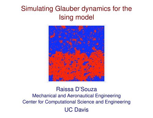
Simulating Glauber dynamics for the Ising model

Simulating Glauber dynamics for the
Ising model
Raissa D’Souza
Mechanical and Aeronautical Engineering
Center for Computational Science and Engineering
UC Davis

Why is it that many materials exhibit “spontaneous
magnetization”?
• At low temperatures, they are magnetic.
• At high temperatures, they are not.

Electron “spins” and magnetization
• W. Lenz (1920) proposed a model of ferromagnetism. That
each electron possesses a “spin”. Parallel spins attract.
Antiparallel spins repel. At sufficiently low temperatures, the
spins should align.
• Ernst Ising (1924), in his doctoral thesis advised by Lenz,
formalized these ideas and examined a 1-D chain of such
spins.
si ∈ {−1, +1}
Ei ∝ −sisj
the “exchange energy”

• Consider a 2-D lattice.
The “Ising” model
• At each site is a spin, si ∈ {−1, +1}.
• Spins interact only with nearest neighbors.
• There can be an external field h.
• Thus the energy for each spin, Ei:
Ei = −
Jijsisj − hsi
{sj}

Total energy, the “Hamiltonian”
H = −
〈i,j〉
Jijsisj −
• The first sum is over all nearest neighbor pairs.
i
hsi
• Jij is the coupling between spins. We take Jij = J = 1.
• Set external field h = 0 (if not, hysteresis).
– Hysteresis enables magnetic storage of data.
– Avalanche phenomena in domain flipping.
– Studied via Random Field Ising Models (RFIM).

• All spins “up” → M = 1.
Magnetization, M
M = 1
N
• All spins “down” → M = −1.
i si

Phase transition in M as function of T
• Peierls (1936), gave a non-rigorous proof that spontaneous
magnetization must exist for the 2-D Ising model.
• Onsager (1944), gave a complete analytic solution.
Phase transitions and universality — more on this later!

How to simulate the Ising model?
• Starting from any initial condition, we know the equilibrium
value of the magnetization. It is a function only of Temperature.
How do we get to equilibrium?
→

Equilibrium
• In equilibrium, Boltzmann probability:
• Ei is energy of state i.
• k is Boltzmann’s constant.
• T is temperature.
p(Ei) = e (−Ei/kT ) /z
• z =
i e−Ei/kT is the partition (i.e., generating) function.

Spin-flip algorithms
“Monte Carlo”
• Use a stream of random numbers to drive a stochastic process,
in this case the generation of a succession of many states of
the spin model.
• For an L × L lattice, there are 2 L×L states. (e.g., If L = 10,
there are 2 100 possible states).
• Want to sample the phase space so that each state occurs with
the same probability as its equilibrium probability.
• Metropolis (1953) detailed balance ensures convergence to
equilibrium.
P (Si)P (Si → Sj) = P (Sj)P (Sj → Si)

Detailed balance
P (Si)P (Si → Sj) = P (Sj)P (Sj → Si)
P (Si→Sj)
P (Sj→Si)
in other words:
= P (Sj)
P (Si)
= e−(Ej−Ei)/kT
(Where the last equality follows from the Boltzmann probability).

Glauber dynamics
• P (Si → Sj) = e −Ej/kT /(e −Ej/kT + e −Ei/kT )
= 1/(1 + e ∆Eji/kT )
• Choose a spin a random.
• Calculate the energy difference resulting if that spin were
flipped: ∆E.
• Transition probability: P (flip) = 1/(1 + e ∆E/kT ).
• Generate a random number, X. If X < P (flip) accept.
• Parameterize time such that one unit of time is N spin-flip
attempts.

Implementing the Glauber dynamics
• Only a finite number (5) of possible energy changes.
• Can pre-compute the probabilities, 1/(1 + e ∆E/kT ).

Simulations
• High temperature (initial condition irrelevant)
• Low temperature (initial condition “quenched”)
• Critical temperature (???)

Issues
• Critical slowing down (correlation length diverges), and so
does the relaxation time....
• The critical point is the most interesting, yet the hardest to
access and pin down!

• “Top” copy all spin up, +1.
A coupled dynamics
• “Bottom” copy all spin down, -1.

Greedy coupled dynamics
• Pick a lattice site, v, at random.
• Calculate probability for spin sv to be +1 in the top, ptop.
• Calculate probability for spin sv to be +1 in the bottom, pbot.

p(+) =
Probabilities (as usual)
e −E(+)β
e −E(+)β + e −E(−)β

Dynamics
• Generate a random number, X.
• set sv to be blue if: X < pbot.
• set sv to be green if: pbot < X < ptop.
• set sv to be yellow if: X > ptop.

The coupled system
Growth of coupling with time.

Online Resources
Ising model simulation:
• http://stp.clarku.edu/simulations/ising2d/
• http://bartok.ucsc.edu/peter/java/ising/keep/ising.html
Cluster-flip dynamics:
• http://www.hermetic.ch/compsci/thesis/chap1.htm