HAND, a new terrain descriptor using SRTM-DEM - DPI - Inpe
HAND, a new terrain descriptor using SRTM-DEM - DPI - Inpe
HAND, a new terrain descriptor using SRTM-DEM - DPI - Inpe

You also want an ePaper? Increase the reach of your titles
YUMPU automatically turns print PDFs into web optimized ePapers that Google loves.
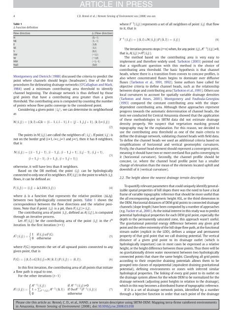
Table 1<br />
Δ Function definition<br />
Flow direction Δ (Flow direction)<br />
N h0,−1i<br />
NE h1,−1i<br />
E h1,0i<br />
SE h1,1i<br />
S h0,1i<br />
SW h−1,1i<br />
W h−1,0i<br />
NW h−1,−1i<br />
Null h0,0i<br />
Montgomery and Dietrich (1988) discussed the criteria to predict the<br />
point where channels should begin (headwater). One of the first<br />
procedures for delineating drainage networks (O'Callaghan and Mark,<br />
1984) used a minimum contributing area threshold to identify<br />
channel beginning. The drainage network is thus defined by those<br />
grid points that have a contributing area greater than a given<br />
threshold. The contributing area is computed by counting the number<br />
of points whose flow paths converge to the considered point.<br />
Considering a given point h i,j i, we can determine its neighborhood<br />
as<br />
Nðhi; jiÞ<br />
¼ fhk; liaGjk ¼ fi1; i; i 1g;<br />
l ¼ fj1; j; j þ 1g;<br />
hk; liphi; jig<br />
ð2Þ<br />
The points in N(hi,ji) are called the neighbors of h i,j i.Ifpointh i,j i is<br />
not on the border grid (i≠1, i≠c, j≠1 andj≠r), then it has 8 neighbors,<br />
that is<br />
Nðhi; jiÞ<br />
¼ fhi1; j 1i; hi 1; ji; hi 1; j þ 1i; hi; j 1i; hi; j þ 1i;<br />
hi þ 1; j 1i; hi þ 1; ji; hi þ 1; j þ 1ig<br />
otherwise, it will have less than 8 neighbors.<br />
Based on the D8 method, the point hi,ji can be hydrologically<br />
connected to only one of its neighbors. If F(hi,ji) is the point to which hi,ji<br />
flows, it can be defined as:<br />
Fðhi; jiÞ<br />
¼hi; jiþDðLDDðhi; jiÞÞ<br />
ð4Þ<br />
where Δ is a function that represents the relative position hΔi,Δji<br />
between two hydrologically connected points. Table 1 shows the<br />
correspondence between the flow directions and the relative positions.<br />
Note that if point hi, ji is a pit, then F(hi, ji)=hi, ji.<br />
The contributing area of point hi, ji, defined as A(hi,ji), is computed<br />
through an iterative process.<br />
Let A t (hi, ji) be the contributing area of the point hi, ji in the t th<br />
iteration. In the first iteration (t=1)<br />
A 1 ðhi; jiÞ<br />
¼<br />
1 ifhi; jigFðGÞ 0 otherwise<br />
where F(G) represents the set of all upward points connected to any<br />
given point, that is<br />
FG ð Þ ¼ fhk; liaGjahi; jiaNðhk; liÞjFðhi;<br />
jiÞ<br />
¼ hk; lig:<br />
ð6Þ<br />
In this first iteration, the contributing area of all points that initiate<br />
a flow path is equal to one.<br />
For the other iterations (tN1)<br />
A t A<br />
ðhi; jiÞ<br />
¼<br />
t 1ðhi; jiÞ<br />
if At 1ðhi; jiÞp0<br />
1 þ P<br />
F−1ðhi;jiÞAt 1ðhk; liÞ<br />
if 0gAt 1 F 1 8<br />
<<br />
ðhi; jiÞ<br />
:<br />
0 otherwise<br />
ARTICLE IN PRESS<br />
4 C.D. Rennó et al. / Remote Sensing of Environment xxx (2008) xxx-xxx<br />
ð3Þ<br />
ð5Þ<br />
ð7Þ<br />
where F − 1 (hi, ji) represents a set of all neighbors of point hi,ji that flow<br />
to it, that is<br />
F 1 ðhi; jiÞ<br />
¼ fhk; liaNðhi; jiÞjFðhk;<br />
liÞ<br />
¼ hi; jig<br />
ð8Þ<br />
The iteration process stops (t=n) when, for any point hi,ji, A t −1 (hi,ji)≠0,<br />
that is, A(hi,ji)=A n (hi,ji).<br />
The method based on the contributing area is very easy to<br />
implement and therefore widely used. Tarboton (2003) pointed out<br />
that a significant question with this method is the choice of<br />
contributing area threshold. The basic hypothesis is that channel<br />
heads, where there is a transition from convex to concave profiles, is<br />
also where concentrated fluxes begins to dominate over diffusive<br />
fluxes (Tarboton et al., 1991, 1992). Some authors have called for<br />
objective criteria to define channel heads, such as the relationship<br />
between slope and contributing area (Tarboton et al., 1991). Others use<br />
local curvatures to account for spatially variable drainage densities<br />
(Tarboton and Ames, 2001). Montgomery and Foufoula-Georgiou<br />
(1993) compared the constant contributing area with the slopedependent<br />
contributing area. Although these approaches represent<br />
progress towards the automatic determination of channel heads, the<br />
tests we conducted for Central Amazonia showed that the application<br />
of these methodologies to <strong>SRTM</strong> data did not estimate drainage<br />
density properly. We suspect that vegetation masking ground<br />
topography may be the explanation. For this reason, we decided to<br />
use the contributing area threshold as one of the main criteria to<br />
define the drainage network, validating channel heads with field data.<br />
To define the channel heads we used an additional criteria based on<br />
simplifications of horizontal and vertical geomorphic curvatures.<br />
Firstly, the channel head element should represent a convergent point,<br />
meaning it should have two or more overland flux paths converging to<br />
it (horizontal curvature). Secondly, the channel profile should be<br />
concave, i.e. where the channel head profile point has a smaller<br />
change of elevation than the mean of the elements located uphill and<br />
downhill of it (vertical curvature).<br />
2.2. The height above the nearest drainage <strong>terrain</strong> <strong>descriptor</strong><br />
To quantify relevant parameters that could uniquely identify generalizable<br />
spatial properties of hill slopes there was the need to have a local<br />
frame of variable topographic reference that should be more useful than<br />
the all encompassing and generic height ASL, or the third dimension in<br />
the <strong>DEM</strong>. Horizontal distances of <strong>DEM</strong> grid points to connected drainage<br />
channels (slope length) have been computed by a number of approaches<br />
(e.g. Tucker et al., 2001). As the initial interest in this study was to predict<br />
potential hydrological properties for each <strong>DEM</strong> grid point, especially the<br />
depth to the permanently saturated zone, this approach wasn't useful.<br />
The gravitational potential energy difference between any given grid<br />
point and the other extremity of the hill slope flow path, at the functional<br />
stream outlet (explicit in the LDD), defines a unique and permanent<br />
property of that grid point that we call draining potential. The vertical<br />
distance of a given grid point to its drainage outlet (which is<br />
hydrologically important) can in most cases be expressed as a relative<br />
height, or the height difference between those points. Thus there will be<br />
no gravitationally driven water movement between two hydrologically<br />
connected points that share the same height. Classifying all grid points<br />
according to their respective draining potentials allows them to be<br />
grouped into classes of equipotential (equivalent draining gravitational<br />
potential), defining environments or zones with inferred similar<br />
hydrological properties. The linking of every grid point to its outlet on<br />
the drainage system allows for the whole <strong>DEM</strong> to be normalized for the<br />
drainage network (adjusting point heights in relation to the drainage),<br />
which in this way becomes a distributed frame of topographic reference.<br />
If D is a set of drainage network points, identified by a number<br />
through a bijective function in order that each point of the drainage<br />
Please cite this article as: Rennó, C. D., et al., <strong>HAND</strong>, a <strong>new</strong> <strong>terrain</strong> <strong>descriptor</strong> <strong>using</strong> <strong>SRTM</strong>-<strong>DEM</strong>: Mapping terra-firme rainforest environments<br />
in Amazonia, Remote Sensing of Environment (2008), doi:10.1016/j.rse.2008.03.018