A very short introduction to Godunov methods

A very short introduction to Godunov methods
Lecture Notes for the COMPSTAR School on Computational
Astrophysics, 8-13/02/10, Caen, France
Olindo Zanotti, Gian Mario Manca
Albert Einstein Institute, Max-Planck-Institute for Gravitational Physics,
Potsdam, Germany
August 10, 2010

Contents
1 Introduction 1
1.1 Conservation form of the 1D Euler equations . . . . . . . . . . . . . 2
1.2 Integral Form of Conservation Laws . . . . . . . . . . . . . . . . . . 2
2 Approximate Riemann solvers for the Euler equations 7
2.1 Approximate State Riemann Solvers . . . . . . . . . . . . . . . . . . 7
2.1.1 “Two-Rarefactions” Riemann Solver . . . . . . . . . . . . . . 7
2.1.2 “All-Shocks” Riemann Solver . . . . . . . . . . . . . . . . . 8
2.2 Approximate Flux Riemann Solvers . . . . . . . . . . . . . . . . . . 8
2.2.1 The HLL(E) Solver . . . . . . . . . . . . . . . . . . . . . . . 8
3 High-Resolution Shock Capturing Methods 11
3.1 Total Variation Diminishing Methods . . . . . . . . . . . . . . . . . . 12
3.2 Reconstruction Procedures . . . . . . . . . . . . . . . . . . . . . . . 12
4 Appendix: Rankine-Hugoniot condition 13
i

Chapter 1
Introduction
A system of equations is in conservative form if it can be written as
with initial and boundary conditions given by
Ut + F(U)x = 0, (1.1)
U(x, 0) = U (0) (x), (1.2)
U(0, t) = UL(t), (1.3)
U(1, t) = UR(t), (1.4)
where U is the vector of conserved variables, while F(U) is the vector of fluxes.
U (0) (x) is the initial data at t = 0; [0, 1] is the spatial domain and boundary conditions
are assumed to be represented by the boundary functions UL(t) and UR(t).
The use of a conservative form of the equations is particularly important when
dealing with problems admitting shocks or other discontinuities in the solution. A nonconservative
numerical method, i.e. a numerical method in which the equations are not
written in a conservative form, might give a numerical solution which looks reasonable
but is incorrect. A well known example is provided by Burger’s equation, i.e. the
momentum equation of an isothermal gas in which pressure gradients are neglected,
and whose non-conservative representation fails dramatically in providing the correct
shock speed if the initial conditions contain a discontinuity (see Leveque 1992, [8]). As
proved by Hou & Le Floch (1994) [6], non conservative schemes do not converge to
the correct solution if a shock wave is present in the flow, whereas, as Lax & Wendroff
(1960) [7] showed in a classical paper, conservative numerical methods, if convergent,
do converge to the weak solution of the problem. On the other hand, it should be
remembered that a conservative formulation and a non-conservative one are equivalent
as long as the solution remains smooth.
1

2 CHAPTER 1. INTRODUCTION
1.1 Conservation form of the 1D Euler equations
The Newtonian hydrodynamics equations for a one-dimensional, non self-gravitating
fluid
∂ρ ∂(ρu)
+ = 0 , (1.5)
∂t ∂x
∂(ρu)
∂t + ∂(ρu2 + p)
= 0 , (1.6)
∂x
∂E
∂t
+ ∂[u(E + p)]
∂x
= 0 , (1.7)
(1.8)
offer a simple example of a system of equations that can be written in conservative
form like in (1.1) with a vector of conserved variables given by
⎡ ⎤
ρ
U = ⎣ ρu
E
⎦ (1.9)
and a flux given by
⎡
F = ⎣
ρu
ρu 2 + p
u(E + p)
⎤
⎦ , (1.10)
where E = 1
2 ρu2 + ρɛ is the total energy, ɛ the specific internal energy. In the case
of the Euler equations the conservative formulation reflects the physical conservation
of specific and well defined quantities, i.e. the mass, the momentum and the energy.
However, for other system of equations it may happen that the conservative formulation
does not reflect any true conserved physical quantity.
1.2 Integral Form of Conservation Laws
Consider a one-dimensional time dependent system described by the Euler equations
written in conservation laws. We can now discretize the spatial domain into N computing
cells Ii = [xi−1/2, xi+1/2] of size ∆x = xi+1/2 − xi−1/2, with i = 1, ..., N.
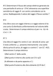
We also define a “control volume” as V ≡ Ii × [tn , tn+1 ] (see Fig. 1.1).
The integral form of the conservative equations (1.1) on this domain can be written
by first integrating (1.1) in space over Ii
d
dt
xi+1/2
x i−1/2
U(x, t)dx = F(U(x i−1/2, t)) − F(U(x i+1/2, t)) , (1.11)
and then in time between t n and t n+1 , with t n < t n+1 to obtain
xi+1/2
x i−1/2
U(x, t n+1 )dx =
xi+1/2
xi−1/2 n+1
t
t n
U(x, t n )dx + (1.12)
F(U(x i−1/2, t))dt −
t n+1
t n
F(U(x i+1/2, t))dt ,

1.2. INTEGRAL FORM OF CONSERVATION LAWS 3
Figure 1.1: Mesh.
which represents the integral form of the equations. At this point we define two new
quantities
U n xi+1/2
1
i =
U(x, t
∆x xi−1/2 n )dt (1.13)
and
such that (1.12) is re-written as
Important remarks:
Fi±1/2 = 1
n+1
t
∆t tn F[U(xi±1/2, t)]dt (1.14)
U n+1
i = U n i + ∆t
∆x (F i−1/2 − F i+1/2). (1.15)
• (1.15) is not yet a numerical scheme. In fact, it has been obtained through mathematical
definitions with no approximations. One should in fact distinguish between
the mathematical formulation of the method, which assumes the knowledge
of the analytic functions U(x, t) and F(x, t), from its numerical application,
which requires an interpretation of the terms entering (1.15) before a
numerical scheme is effectively built.
• (1.15) becomes a numerical scheme, and indeed it is called “Godunov scheme”,
when approximation are introduced for the computations of the numerical fluxes
F i−1/2 and an interpretation is given to the averages Ui.
• In Godunov’s first order method the evolution from the time t n to the time
t n+1 = t n + ∆t is obtained by first assuming a piece-wise constant distribution
of the data over the spatial grid, i.e. by assuming that Ui are constant (see
Fig.1.2). Of course, by doing so, part of the knowledge of the original initial data
U(x, t n ) inside the cell is lost, and to increase the spatial accuracy a number of
reconstruction procedures has been developed.

4 CHAPTER 1. INTRODUCTION
• Different numerical algorithms can then be devised from (1.15) according to
the method used to calculate the fluxes at each interface, F i−1/2 and F i+1/2.
At the interface between adjacent numerical cells the quantity Ui manifests a
jump, thus generating a sequence of local Riemann problems. Hence, we say
that (1.15) is Godunov’s first-order upwind method if the fluxes are calculated
by solving such sequence of local Riemann problems. The left and right states
are the same piece wise constant distribution of data given by (1.13). Solving
the local Riemann problem provides either the term U(x i±1/2, t) to be used in
(1.14), or the F[U(x i±1/2, t)] term itself.
• Finally, it should be recalled that the Godunov scheme (1.15) with the piece wise
constant distribution of the data is just first order accurate in time and space. This
can be better appreciated if we apply the scheme (1.15) to the linear advection
equation with the flux given by F = λU. In this case the solution of each local
Riemann problem at the generic cell interface xi+1/2 is given by Un i , if λ < 0,
, if λ > 0. Therefore, the resulting scheme is given by
and by U n i+1
and
U n+1
i = Un i − c(U n i − U n i−1), if λ > 0, (1.16)
U n+1
i = Un i − c(U n i+1 − U n i ), if λ < 0, (1.17)
where c = λ∆t/∆x is the Courant factor. The schemes (1.16) and (1.17)
are nothing but the first order upwind method first introduced by Courant et al.
(1952). The spatial accuracy of the first order Godunov’s method presented here
can be improved by adopting some kind of reconstruction procedure, while the
time accuracy can be increased by combining the method outlined above with a
conservative Runge-Kutta scheme.
• A final remark about the scheme (1.15) is that the time step ∆t must satisfy a
Courant-Friedrich-Lewy type condition (Courant et al. 1928)
∆t ≤ ∆x
|vn , (1.18)
max|
where v n max denotes the maximum wave velocity 1 present through the computational
domain at time t n .
It should be emphasized that the originality of Godunov’s idea consists of the way
an upwind method is obtained for a general nonlinear system of equations. Upwind
methods, we recall, are characterized by the fact that the spatial differencing is performed
using grid points on the side from which information flows. If we think of
the advection equation as modelling the advection of a concentration profile in a fluid
stream, then this is exactly the upwind direction. For a linear system of equations, upwind
methods can only be used if all the eigenvalues of the matrix F have the same sign.
1Note that in a Riemann problem both shock waves and rarefaction waves are produced, so one has
to look for the fastest wave at each time step. In multidimensional problems, when this procedure might
become unsuitable, a common alternative is to select vn max as vn max = max(|vn i | + an i ), where vn i is the
flow velocity and an i is the sound speed.

1.2. INTEGRAL FORM OF CONSERVATION LAWS 5
U
i−1 i
i+1
Local Riemann Problem
Interface
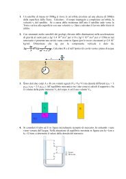
Figure 1.2: Schematic representation of a piece-wise constant distribution of a general
quantity U giving rise to a sequence of local Riemann problems at the interface
between adjacent cells.
If the eigenvalues have mixed signs, an alternative procedure is often adopted aimed at
identifying the direction of propagation of information on the numerical grid. According
to this procedure, the flux F is decomposed in two parts, F + and F − , in such a way
that the corresponding Jacobian matrices F + = ∂F + /∂U and F − = ∂F − /∂U contain
just the positive and negative eigenvalues, respectively, of the original matrix F.
The upwind character of the resulting numerical methods, called Flux Vector Splitting
methods (FVS), is thus guaranteed. However, for nonlinear systems of equations the
matrix of eigenvectors is not constant, and this same approach does not apply directly.
Godunov succeeded in obtaining an upwind method in which the local characteristic
structure is not provided by diagonalizing the Jacobian matrix, but rather by solving a
Riemann problem forward in time. The solutions of Riemann problems, in fact, provide
the necessary information about the characteristic structure, and lead to conservative
methods, since they are themselves solution of the conservation laws.
x

6 CHAPTER 1. INTRODUCTION

Chapter 2
Approximate Riemann solvers
for the Euler equations
Godunov’s method, and its higher order modifications, require the solution of the Riemann
problem at every cell boundary and on each time level. This amounts to calculating
the solution in the regions that form behind the non-linear waves developing in
the Riemann problem (as shown in Fig. 2.1) as well as the wave speeds necessary for
deriving the complete wave structure of the solution.
The solution of the general Riemann problem cannot be given in a closed analytic
form, even for one dimensional Newtonian flows. What can be done is to find the answer
numerically to any required accuracy, and in this sense the Riemann problem is
said to have been solved exactly, even though the actual solution is not analytical. In
Newtonian hydrodynamics, the exact solution of the one dimensional Riemann problem
was found by Courant & Friedrichs (1948).
Approximate Riemann solvers can be divided in approximate State Riemann Solvers,
where an approximation is given to the state U(x i±1/2, t) which is then used to evaluate
the corresponding flux by (1.14), and in approximate Flux Riemann Solvers, where
an approximation is given to the flux directly, thus avoiding the computation of the
state U(x i±1/2, t) at each zone edge.
2.1 Approximate State Riemann Solvers
2.1.1 “Two-Rarefactions” Riemann Solver
Finding the wave pattern in a Riemann problem is part of the solution procedure, but
if one assumes a priori that both nonlinear waves are rarefactions, then the solution
can be obtained analytically (see Toro (1997) for the Newtonian case and [11] for
the relativistic case). The resulting method is very accurate for flow conditions near
vacuum, when rarefaction waves give indeed the best approximation to the problem.
7

8CHAPTER 2. APPROXIMATE RIEMANN SOLVERS FOR THE EULER EQUATIONS
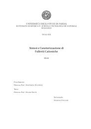
Figure 2.1: Riemann problem for the 3D Euler equation: u is the fluid speed, a is
the sound speed. The 1D case can be recovered simply disregarding the tangential
velocities in the y and z direction v and w starting from an initial condition in which
they are zero on both sides of the discontinuity. The variables ρ and p represent density
and pressure respectively.
Figure 2.2: Control volume for the computation of the approximate HLLE flux.
2.1.2 “All-Shocks” Riemann Solver
In analogy with the previous solver, it is possible to ignore the occurrence of rarefaction
waves and assume that both nonlinear waves are shock waves. This represents a
good approximation in a wide range of flow conditions, particularly when dealing with
more complicated equations of state than the usual polytropic one (see Colella, 1982).
However, this approach is typically inadequate in the case of a transonic rarefaction,
yielding a numerical solution which does not satisfy the entropy condition.
2.2 Approximate Flux Riemann Solvers
2.2.1 The HLL(E) Solver
In the Riemann solver given by Harten, Lax and van Leer (1983) and later improved
by Einfeldt (1988), ie the HLLE approximate-flux Riemann solver or simply HLLE
Riemann solver, it is assumed that, after the decay of the initial discontinuity of the
local Riemann problem, only two waves propagate in two opposite directions with

2.2. APPROXIMATE FLUX RIEMANN SOLVERS 9
velocities SL and SR, generating a single state between them, i.e.
⎧
⎨
U =
⎩
UL if x/t < SL,
U HLLE
if SL < x/t < SR,
UR if x/t > SR,
where SL and SR are the smallest and the largest of the signal speeds arising from the
solution of the Riemann problem1 .
We will now show how to compute U HLLE
. The time integral form of Eq. (1.10 on
the control volume defined in Fig. 2.2 is:
xR
xR
T
T
U(x, T )dx = U(x, 0)dx + F(U(xL, t))dt − F(U(xR, t))dt.
xL
xL
0
0
(2.1)
The evaluation of the right-hand side gives a consistency condition:
xR
xL
U(x, T )dx = xRUR − xLUL + T (FL − FR) (2.2)
where FL = F(UL) and FR = F(UR). Now we split the the integral on the left-hand
side of Eq. (2.1) into three integrals
xR
xL
U(x, T )dx =
T SL
xL
T SR
xR
U(x, T )dx + U(x, T )dx + U(x, T )dx
T SL
T SR
and evaluate the first and third terms on the right-hand side. We obtain:
xR
xL
U(x, T )dx =
T SR
T SL
Comparing Eq. (2.2) with Eq. (2.3) gives
T SR
T SL
U(x, T )dx + (T SL − xL)UL + (xR − T SR)UR (2.3)
U(x, T )dx = T (SUR − SLUL + FL − FR) (2.4)
Dividing by the length T (SR − SL) we finally obtain:
U HLLE
T SR
1
=
U(x, T )dx =
T (SR − SL) T SL
(SUR − SLUL + FL − FR)
(SR−SL).
(2.5)
Thus the integral average of the exact solution of the Riemann problem between the
slowest and the fastest signals at time T is a known constant, provided that the signal
1 The simplest choice is to take the smallest and the largest among the eigenvalues of the Jacobian matrix
∂F/∂U evaluated at some intermediate state. For the 1D Euler equation the simplest estimate proposed by
Davis in [12] would be SL = ul − al and SR = ur + ar, where the u’s are the fluid velocities and the a’s
the sound speeds on the left and on the right of the initial discontinuity respectively.

10CHAPTER 2. APPROXIMATE RIEMANN SOLVERS FOR THE EULER EQUATIONS
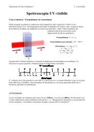
Figure 2.3: Approximate state for HLLE: the integral average of the exact solution of
the Riemann problem between the slowest and the fastest signals at a given time T is a
known constant, provided that the signal speeds SL and SR are known; such constants
is the right-hand side of Eq. (2.5).
speeds SL and SR are known; such constants is the right-hand side of Eq. (2.5) and we
denote it by
U HLLE
= SRUR − SLUL + FL − FR
(2.6)
SR − SL
We now apply the Rankine-Hugoniot conditions (see Appendix 4) across the left and
the right waves, to obtain
F HLLE
F HLLE
= FL + SL(U HLLE
= FR + SR(U HLLE
− UL) (2.7)
− UR) (2.8)
Finally, by replacing (2.6) into (2.7) or into (2.8) we obtain the HLLE flux to be used
in the Godunov scheme
F HLLE
= SRFL − SLFR + SLSR(UR − UL)
. (2.9)
SR − SL
This Riemann solver, which is very simple in its original form, performs well at critical
sonic rarefactions but produces excessive smearing at contact discontinuities due to
the fact that middle waves are ignored in the solution. Furthermore, it needs to be
implemented with an algorithm for the calculation of the wave speeds SL and SR.

Chapter 3
High-Resolution Shock
Capturing Methods
A large effort has been spent in recent years in developing a numerical method able to
satisfy the following requirements
• at least second order accuracy on smooth parts of the solution,
• sharp resolution of discontinuities without large smearing,
• absence of spurious oscillations everywhere in the solution,
• converge to the “true” solution as the grid is refined.
Irrespective of the Riemann solver adopted, the original Godunov method is only
first order accurate on smooth solutions and gives poor approximations to shock waves
and other discontinuities. However, if we wanted to modify the first order Godunov
method in order to obtain a higher order numerical scheme we would encounter a
fundamental difficulty. Namely, all higher order linear schemes produce nonphysical
oscillations in the vicinity of large gradients. If we define a monotone linear scheme
of the form u n+1
i = H(un i−l , ..., uni+r ), where H is a linear operator, as a scheme
for which ∂H/∂un k ≥ 0 for all k, then only monotone linear schemes do not suffer
from oscillations. Unfortunately, as proved by Godunov (1959), monotone schemes
are at most first order accurate. As a result, higher order linear schemes and absence of
oscillations are two incompatible requirements, forcing the use of nonlinear numerical
methods. To summarize: HRSC methods result from the combination of Godunov
type methods, which take advantage of the conservation form of the equations, and of
numerical techniques aimed at obtaining second order (or higher) accuracy in smooth
parts of the solution without producing oscillations.
11

12 CHAPTER 3. HIGH-RESOLUTION SHOCK CAPTURING METHODS
3.1 Total Variation Diminishing Methods
The concept of spurious oscillations in the solution can be made more quantitative by
the notion of the total variation of the solution. The total variation of a grid function
Q at time level t n is defined as
T V (Q n ) ≡
+∞
i=−∞
|Q n i − Q n i−1|, (3.1)
and is used to “measure” the oscillations appearing in a numerical solution. The requirement
to have a scheme that is both second (or higher) order accurate and does not
produce spurious oscillations is that the total variation should not be increasing in time,
so that the total variation at any time is uniformly bounded by the total variation of the
initial data. In other words, a numerical method is said to be total variation diminishing
(TVD) if, for any set of data Q n , the values Q n+1 computed by the method satisfy
T V (Q n+1 ) ≤ T V (Q n ). (3.2)
TVD schemes are intimately linked to the more traditional Artificial Viscosity methods
(see Richtmyer & Morton, 1967), where viscous terms were introduced explicitly in the
scheme in order to eliminate or at least control the appearance of the oscillations. In
modern TVD methods, on the contrary, artificial viscosity is inherent to the scheme
itself in a rather sophisticated way. TVD methods do not generally extend beyond
second order accuracy. To construct third (and higher) order methods one must drop
condition (3.2) and allow for an increase of the total variation which is proportional
to some power of the typical step size. The resulting methods are called Essentially
Non-Oscillatory (ENO) (see Toro, 1997).
3.2 Reconstruction Procedures
Due to the discrete numerical representation, any information about the behavior of the
quantities inside the numerical cell is lost. In order to recover in part this information
and improve the spatial accuracy of a numerical code based on Riemann solvers, different
spatial reconstruction procedures have been developed. The common goal is to
interpolate the profiles of the various thermodynamical quantities within each cell, thus
providing a better estimate for the calculation of the left and of the right state of the
Riemann problem to be solved at the interface between two adjacent cells.
Van Leer (1979) was the first to introduce the idea of modifying the piece-wise
constant data (1.13) as a first step in achieving higher order spatial accuracy. This approach
has been generically called Monotone Upstream-centered Scheme for Conservation
Laws (MUSCL). Since then, many other reconstruction procedures have been
developed, such as the piece-wise parabolic method (PPM) of Colella & Woodward
(1984), or the piece-wise hyperbolic (PHM) method of Marquina (1994), where the
interpolation is obtained by using hyperbolae instead of parabolae.

Chapter 4
Appendix: Rankine-Hugoniot
condition
The integral form of Eq. (1.1) on the interval [xL, xR] at time t is
d
dt
xR
xL
U(x, t)dx = F(U(xL, t)) − F(U(xR, t)) (4.1)
We recall a simple formula to compute the derivative of an integral:
x2(t)
x2(t)
d
∂f(x, t)
f(x, t)dx =
dx + f(x2(t), t)
dt x1(t)
x1(t) ∂t
dx2(t)
dt − f(x1(t), t) dx1(t)
.
dt
(4.2)
If a discontinuity is present in the solution (see Fig. 2.2) and propagating along s(t) we
can split the left-hand side of Eq. (4.1) in the following way:
d
dt
s(t)
xL
U(x, t)dx + d
xR
U(x, t)dx = F(U(xL, t)) − F(U(xR, t)) (4.3)
dt s(t)
Applying formula (4.2) to Eq. (4.3) gives:
s(t)
xR
∂U(x, t) ∂U(x, t)
F(U(xL, t))−F(U(xR, t)) = [U(sL, t)−U(sR, t)]S+
dx+
dx
xL ∂t
s(t) ∂t
(4.4)
where S = ds(t)
dt and U(sL, t) and U(sR, t) are the left and right limit of U(x, t) for
x → s(t).
When xL → s(t) and xR → s(t) the two integrals on the right-hand side of
Eq. (4.4) vanish and we finally obtain the Rankine-Hugoniot condition
F(U(sL, t)) − F(U(sR, t)) = [U(sL, t) − U(sR, t)]S (4.5)
which connects states and fluxes across a discontinuity.
13

14 CHAPTER 4. APPENDIX: RANKINE-HUGONIOT CONDITION

Bibliography
[1] Colella, P., 1982, SIAM J. Sci. Stat. Comput., 3, 76.
[2] Courant, R., Friedrichs, K. O., Lewy, H., 1928, Math. Ann., 100, 32
[3] Courant, R., Isaacson, E., Rees, M., 1952, Comm. Pure Appl. Math., 5, 243.
[4] Einfeldt, B., 1988, SIAM J. Num. Anal., 25, 294.
[5] Harten, A., Lax, P. D., van Leer, B., 1983, SIAM Reviews, 25, 35.
[6] Hou, T. Y., LeFloch, P., 1994, Math. of Comput., 62, 497.
[7] Lax, P. D., Wendroff, B., 1960, Comm. Pure Appl. Math., XVII, 381.
[8] Leveque, R. J. 1992, Numerical Methods for Conservation Laws, Birkhauser
[9] Leveque, R. J., Mihalas, D., Dorfi, E. A., Müller, E., 1998, Computational
Methods for Astrophysical Fluid Flows Saas-Fee Advanced Course 27, Springer
[10] Martí, J.M. & Müller, E. 1994, J. Fluid Mech., 258, 317.
[11] Rezzolla, L. & Zanotti, O. 2001, J. Fluid Mech. 449, 395.
[12] S. F. Davis, SIAM J.Sci.Stat.Comput.,9:445-473,1988
[13] Toro, E. 1997, Riemann Solvers and Numerical Methods for Fluid Dynamics,
Springer.
15