Polyharmonic boundary value problems
Polyharmonic boundary value problems
Polyharmonic boundary value problems

You also want an ePaper? Increase the reach of your titles
YUMPU automatically turns print PDFs into web optimized ePapers that Google loves.
Filippo Gazzola<br />
Hans-Christoph Grunau<br />
Guido Sweers<br />
<strong>Polyharmonic</strong> <strong>boundary</strong> <strong>value</strong><br />
<strong>problems</strong><br />
A monograph on positivity preserving and<br />
nonlinear higher order elliptic equations in<br />
bounded domains<br />
Springer
Dedicated to our wives Chiara, Brigitte and Barbara.<br />
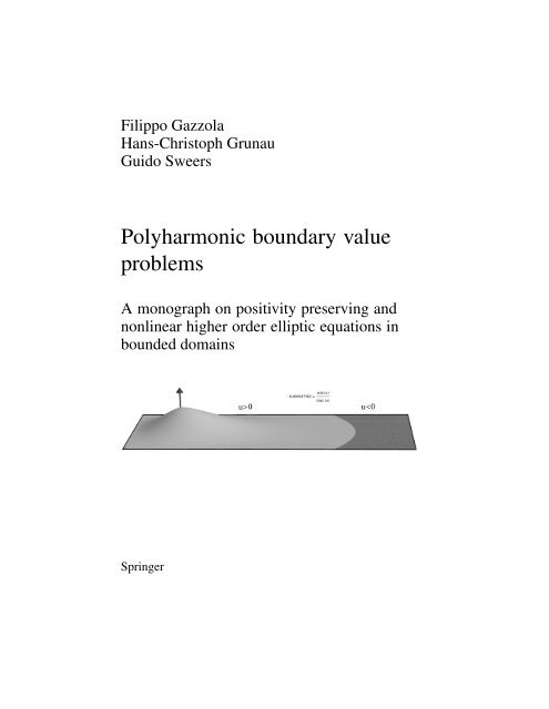
The cover figure displays the solution of ∆ 2 u = f in a rectangle with homogeneous<br />
Dirichlet <strong>boundary</strong> condition for a nonnegative function f with its support concentrated<br />
near a point on the left hand side. The dark part shows the region where u < 0.
Preface<br />
Linear elliptic equations arise in several models describing various phenomena in<br />
the applied sciences, the most famous being the second order stationary heat equation<br />
or, equivalently, the membrane equation. For this intensively well-studied linear<br />
problem there are two main lines of results. The first line consists of existence and<br />
regularity results. Usually the solution exists and “gains two orders of differentiation”<br />
with respect to the source term. The second line contains comparison type<br />
results, namely the property that a positive source term implies that the solution<br />
is positive under suitable side constraints such as homogeneous Dirichlet <strong>boundary</strong><br />
conditions. This property is often also called positivity preserving or, simply,<br />
maximum principle. These kinds of results hold for general second order elliptic<br />
<strong>problems</strong>, see the books by Gilbarg-Trudinger [197] and Protter-Weinberger [346].<br />
For linear higher order elliptic <strong>problems</strong> the existence and regularity type results remain,<br />
as one may say, in their full generality whereas comparison type results may<br />
fail. Here and in the sequel “higher order” means order at least four.<br />
Most interesting models, however, are nonlinear. By now, the theory of second<br />
order elliptic <strong>problems</strong> is quite well developed for semilinear, quasilinear and even<br />
for some fully nonlinear <strong>problems</strong>. If one looks closely at the tools being used in<br />
the proofs, then one finds that many results benefit in some way from the positivity<br />
preserving property. Techniques based on Harnack’s inequality, De Giorgi-Nash-<br />
Moser’s iteration, viscosity solutions etc., all use suitable versions of a maximum<br />
principle. This is a crucial distinction from higher order <strong>problems</strong> for which there is<br />
no obvious positivity preserving property. A further crucial tool related to the maximum<br />
principle and intensively used for second order <strong>problems</strong> is the truncation<br />
method, introduced by Stampacchia. This method is helpful in regularity theory, in<br />
properties of first order Sobolev spaces and in several geometric arguments, such<br />
as the moving planes technique which proves symmetry of solutions by reflection.<br />
Also the truncation (or reflection) method fails for higher order <strong>problems</strong>. For instance,<br />
the modulus of a function belonging to a second order Sobolev space may<br />
not belong to the same space. The failure of maximum principles and of truncation<br />
methods, one could say, are the main reasons why the theory of nonlinear higher<br />
order elliptic equations is by far less developed than the theory of analogous second<br />
v
vi Preface<br />
order equations. On the other hand, in view of many applications and increasing interest<br />
especially in the last twenty years, one should try to develop new tools suitable<br />
for higher order <strong>problems</strong> involving polyharmonic operators.<br />
The simple example of the two functions x ↦→ ±|x| 2 shows that already for the biharmonic<br />
operator the standard maximum principle fails. Nevertheless, taking also<br />
<strong>boundary</strong> conditions into account could yield comparison or positivity preserving<br />
properties and indeed, in certain special situations, such behaviour can be observed.<br />
It is one goal of the present exposition to describe situations where positivity preserving<br />
properties hold true or fail, respectively, and to explain how we have tackled<br />
the main difficulties related to the lack of a general comparison principle. In the<br />
present book we also show that in many higher order <strong>problems</strong> positivity preserving<br />
“almost” occurs. By this we mean that the solution to a problem inherits the sign<br />
of the data, except for some small contribution. By the experience from the present<br />
work, we hope that suitable techniques may be developed in order to obtain results<br />
quite analogous to the second order situation. Many recent higher order results give<br />
support to this hope.<br />
A further goal of the present book is to collect some of those <strong>problems</strong>, where the<br />
authors were particularly involved, and to explain by which new methods one can<br />
replace second order techniques. In particular, to overcome the failure of the maximum<br />
principle and of the truncation method several ad hoc ideas will be introduced.<br />
Let us now explain in some detail the subjects we address within this book.<br />
Linear higher order elliptic <strong>problems</strong><br />
The polyharmonic operator (−∆) m is the prototype of an elliptic operator L of order<br />
2m, but with respect to linear questions, much more general operators can be considered.<br />
A general theory for <strong>boundary</strong> <strong>value</strong> <strong>problems</strong> for linear elliptic operators<br />
L of order 2m was developed by Agmon-Douglis-Nirenberg [4, 5, 6, 148]. Although<br />
the material is quite technical, it turns out that the Schauder theory as well as the<br />
L p -theory can be developed to a large extent analogously to second order equations.<br />
The only exception are maximum modulus estimates which, for linear higher order<br />
<strong>problems</strong>, are much more restrictive than for second order <strong>problems</strong>. We provide a<br />
summary of the main results which hopefully will prove to be sufficiently wide to<br />
be useful for anybody who needs to refer to linear estimates or existence results.<br />
The main properties of higher – at least second – order Sobolev spaces will be<br />
recalled. Since more orders of differentiation are involved, several different equivalent<br />
norms are available in these spaces. A crucial role in the choice of the norm<br />
is played by the regularity of the <strong>boundary</strong>. For the second order Dirichlet problem<br />
for the Poisson equation a nonsmooth <strong>boundary</strong> leads to technical difficulties but,<br />
due to the maximum principle, there is an inherent stability so that, when approximating<br />
nonsmooth domains by smooth domains, one recovers most of the features<br />
for domains with smooth <strong>boundary</strong>, see [46]. For Neumann <strong>boundary</strong> conditions<br />
the situation is more complicated in domains with rather wild boundaries, although
Preface vii<br />
even for polygonal boundaries they do not show spectacular changes. For higher<br />
order <strong>boundary</strong> <strong>value</strong> <strong>problems</strong> some peculiar phenomena occur. For instance, the<br />
so-called Babuˇska and Sapondˇzyan paradoxes [28, 357] forces one to be very careful<br />
in the choice of the norm in second order Sobolev spaces since some <strong>boundary</strong><br />
<strong>value</strong> <strong>problems</strong> strongly depend on the regularity of the <strong>boundary</strong>. This phenomenon<br />
and its consequences will be studied in some detail.<br />
Positivity in higher order elliptic <strong>problems</strong><br />
As long as existence and regularity results are concerned, the theory of linear higher<br />
order <strong>problems</strong> is already quite well developed as explained above. This is no longer<br />
true as soon as qualitative properties of the solution related to the source term are<br />
investigated. For instance, if we consider the clamped plate equation<br />
∆ 2 u = f in Ω,<br />
u = ∂u<br />
∂ν = 0 on ∂Ω,<br />
(0.1)<br />
the “simplest question” seems to find out whether the positivity of the datum implies<br />
the positivity of the solution, Or, physically speaking,<br />
does upwards pushing of a clamped plate yield upwards bending?<br />
Equivalently, one may ask whether the corresponding Green function G is positive.<br />
In some special cases, the answer is “yes”, while it is “no” in general. However,<br />
in numerical experiments, it appears very difficult to display the negative part and<br />
heuristically, one feels that the negative part of G – if present at all – is small in a<br />
suitable sense compared with the “dominating” positive part. We discuss not only<br />
the cases where one has positive Green functions and develop a perturbation theory<br />
of positivity, but we shall also discuss systematically under which conditions one<br />
may expect the negative part of the Green function to be small. We expect such<br />
smallness results to have some impact on future developments in the theory of nonlinear<br />
higher order elliptic <strong>boundary</strong> <strong>value</strong> <strong>problems</strong>.<br />
Boundary conditions<br />
For second order elliptic equations one usually extensively studies the case of<br />
Dirichlet <strong>boundary</strong> conditions because other <strong>boundary</strong> conditions do not exhibit<br />
too different behaviours. For the biharmonic equation ∆ 2 u = f in a bounded domain<br />
of R n it is not at all obvious which <strong>boundary</strong> condition would serve as a role<br />
model. Then a good approach is to focus on some <strong>boundary</strong> conditions that describe<br />
physically relevant situations. We consider a simplified energy functional and derive<br />
its Euler-Lagrange equation including the corresponding natural <strong>boundary</strong> conditions.<br />
We start with the linearised model for the beam. From a physical point of
viii Preface<br />
view, as long as the fourth order planar equation is considered, the most interesting<br />
seem to be not only the Dirichlet <strong>boundary</strong> conditions but also the Navier or<br />
Steklov <strong>boundary</strong> conditions. The Dirichlet conditions correspond to the clamped<br />
plate model whereas Navier and Steklov conditions correspond to the hinged plate<br />
model, either by neglecting or considering the contribution of the curvature of the<br />
<strong>boundary</strong>. Each one of these <strong>boundary</strong> conditions requires the unknown function<br />
to vanish on the <strong>boundary</strong>, the difference being on the second <strong>boundary</strong> condition.<br />
These three <strong>boundary</strong> conditions have their own features and none of them may be<br />
thought to play the model role. We discuss all of them and emphasise their own peculiarities<br />
with respect to the comparison principles, to their variational formulation<br />
and to solvability of related nonlinear <strong>problems</strong>.<br />
Eigen<strong>value</strong> <strong>problems</strong><br />
For second order <strong>problems</strong>, such as the Dirichlet problem for the Laplace operator,<br />
one has not only the existence of infinitely many eigen<strong>value</strong>s but also the simplicity<br />
and the one sign property of the first eigenfunction. For the biharmonic Dirichlet<br />
problem, this property is true in a ball but it is false in general. Again, a crucial role<br />
is played by the sign of the corresponding Green function. Concerning the isoperimetric<br />
properties of the first eigen<strong>value</strong> of the Dirichlet-Laplacian, the Faber-Krahn<br />
[162, 253, 254] result states that, among domains having the same finite volume it<br />
attains its minimum when the domain is a ball. A similar result was conjectured to<br />
hold for the biharmonic operator under homogeneous Dirichlet <strong>boundary</strong> conditions<br />
by Lord Rayleigh [350] in 1894. Although this statement has been proved only in<br />
domains of dimensions n = 2,3, it is the common feeling that it should be true in<br />
any dimension. The minimisation of the first Steklov eigen<strong>value</strong> appears to be less<br />
obvious. And, indeed, we will see that a Faber-Krahn type result does not hold in<br />
this case.<br />
Semilinear equations<br />
Among nonlinear <strong>problems</strong> for higher order elliptic equations one may just mention<br />
models for thin elastic plates, stationary surface diffusion flow, the Paneitz-Branson<br />
equation and the Willmore equation as frequently studied. In membrane biophysics<br />
the Willmore equation is also known as Helfrich model [227]. Moreover, several<br />
results concerning semilinear equations with power type nonlinear sources are also<br />
extremely useful in order to understand interesting phenomena in functional analysis<br />
such as the failure of compactness in the critical Sobolev embedding and in related<br />
inequalities.<br />
One further motivation to study nonlinear higher order elliptic reaction-diffusion<br />
type equations like
Preface ix<br />
(−∆) m u = f (u) (∗)<br />
in bounded domains is to understand whether the results available in the simplest<br />
case m = 1 can also be proved for any m, or whether the results for m = 1 are special,<br />
in particular as far as positivity and the use of maximum principles are concerned.<br />
The differential equation (∗) is complemented with suitable <strong>boundary</strong> conditions. As<br />
already mentioned above, if m = n = 2, equation (∗) may be considered as a nonlinear<br />
plate equation for plates subject to nonlinear feedback forces, one may think<br />
e.g. of suspension bridges. In this case, (∗) may also be interpreted as a reactiondiffusion<br />
equation, where the diffusion operator ∆ 2 refers to (linearised) surface<br />
diffusion.<br />
The first part of Chapter 7 is devoted to the proof of symmetry results for positive<br />
solutions to (∗) in the ball under Dirichlet <strong>boundary</strong> conditions. As already<br />
mentioned, truncation and reflection methods do not apply to higher order <strong>problems</strong><br />
so that a suitable generalisation of the moving planes technique is needed here.<br />
Equation (∗) deserves a particular attention when f (u) has a power-type behaviour.<br />
In this case, a crucial role is played by the critical power s = (n+2m)/(n−<br />
2m) which corresponds to the critical (Sobolev) exponent which appears whenever<br />
n > 2m. Indeed, subcritical <strong>problems</strong> in bounded domains enjoy compactness properties<br />
as a consequence of the Rellich-Kondrachov embedding theorem. But compactness<br />
is lacking when the critical growth is attained and by means of Pohoˇzaevtype<br />
identities, this gives rise to many interesting phenomena. The existence theory<br />
can be developed similarly to the second order case m = 1 while it becomes immediately<br />
quite difficult to prove positivity or nonexistence of certain solutions.<br />
Nonexistence phenomena are related to so-called critical dimensions introduced by<br />
Pucci-Serrin [347, 348]. They formulated an interesting conjecture concerning these<br />
critical dimensions. We give a proof of a relaxed form of it in Chapter 7. We also<br />
give a functional analytic interpretation of these nonexistence results, which is reflected<br />
in the possibility of adding L 2 –remainder terms in Sobolev inequalities with<br />
critical exponent and optimal constants. Moreover, the influence of topological and<br />
geometrical properties of Ω on the solvability of the equation is investigated. Also<br />
applications to conformal geometry, such as the Paneitz-Branson equation, involve<br />
the critical Sobolev exponent since the corresponding semilinear equation enjoys<br />
a conformal covariance property. In this context a key role is played by a fourth<br />
order curvature invariant, the so-called Q-curvature. Our book does not aim at giving<br />
an overview of this rapidly developing subject. For this purpose we refer to the<br />
monographs of Chang [89] and Druet-Hebey-Robert [149]. We want to put a spot<br />
on some special aspects of such kind of equations. First, we consider the question<br />
whether in suitable domains in euclidean space it is possible to change the euclidean<br />
background metric conformally into a metric which has strictly positive constant Qcurvature,<br />
while at the same time, certain geometric quantities vanish on the <strong>boundary</strong>.<br />
Secondly, we study a phenomenon of nonuniqueness of complete metrics in hyperbolic<br />
space, all being conformal to the Poincaré-metric and all having the same<br />
constant Q-curvature. This result is in strict contrast with the corresponding problem<br />
involving constant negative scalar curvature.
x Preface<br />
We conclude the discussion of semilinear elliptic <strong>problems</strong> with some observations<br />
on fourth order <strong>problems</strong> with supercritical growth. Corresponding second<br />
order results heavily rely on the use of maximum principles and constructions of<br />
many refined auxiliary functions having some sub- or supersolution property. Such<br />
techniques are not available at all for the fourth order <strong>problems</strong>. In symmetric situations,<br />
however, they could be replaced by different tools so that many of the results<br />
being well established for second order equations do indeed carry over to the fourth<br />
order ones.<br />
A Dirichlet problem for Willmore surfaces of revolution<br />
A frame invariant modeling of elastic deformations of surfaces like thin plates or<br />
biological membranes gives rise to variational integrals involving curvature and area<br />
terms. A special case is the Willmore functional<br />
<br />
H 2 dω,<br />
Γ<br />
which up to a <strong>boundary</strong> term is conformally invariant. Here H denotes the mean<br />
curvature of the surface Γ in R 3 . Critical points of this functional are called<br />
Willmore surfaces, the corresponding Euler-Lagrange equation is the so-called<br />
Willmore equation. It is quasilinear, of fourth order and elliptic. While a number<br />
of beautiful results have been recently found for closed surfaces, see e.g.<br />
[35, 156, 262, 263, 264, 371], only little is known so far about <strong>boundary</strong> <strong>value</strong> <strong>problems</strong><br />
since the difficulties mentioned earlier being typical for fourth order <strong>problems</strong><br />
due to a lack of maximum principles add here to the difficulty that the ellipticity<br />
of the equation is not uniform. The latter reflects the geometric nature of the equation<br />
and gives rise e.g. to the problem that minimising sequences for the Willmore<br />
functional are in general not bounded in the Sobolev space H 2 . In this book we<br />
confine ourselves to a very special situation, namely the Dirichlet problem for symmetric<br />
Willmore surfaces of revolution. Here, by means of some refined geometric<br />
constructions, we succeed in considering minimising sequences of the Willmore<br />
functional subject to Dirichlet <strong>boundary</strong> conditions and with suitable additional C 1 -<br />
properties thereby gaining weak H 2 - and strong C 1 -compactness. We expect the<br />
theory of <strong>boundary</strong> <strong>value</strong> <strong>problems</strong> for Willmore surfaces to develop rapidly and<br />
consider this chapter as one contribution to outline directions of possible future research<br />
in quasilinear geometric fourth order equations.
Acknowledgements<br />
The authors are grateful to their colleagues, friends, and collaborators Gianni Arioli,<br />
Elvise Berchio, Francisco Bernis, Isabeau Birindelli, Dorin Bucur, Daniele<br />
Cassani, Philippe Clément, Anna Dall’Acqua, Cesare Davini, Klaus Deckelnick,<br />
Alberto Ferrero, Steffen Fröhlich, Maurizio Grasselli, Gerhard Huisken, Paschalis<br />
Karageorgis, Bernd Kawohl, Marco Kühnel, Ernst Kuwert, Monica Lazzo, Andrea<br />
Malchiodi, Joseph McKenna, Christian Meister, Erich Miersemann, Enzo Mitidieri,<br />
Serguei Nazarov, Mohameden Ould Ahmedou, Vittorino Pata, Dario Pierotti, Wolfgang<br />
Reichel, Frédéric Robert, Bernhard Ruf, Edoardo Sassone, Reiner Schätzle,<br />
Friedhelm Schieweck, Paul G. Schmidt, Marco Squassina, Franco Tomarelli, Wolf<br />
von Wahl, and Tobias Weth for inspiring discussions and sharing ideas.<br />
Essential parts of the book are based on work published in different form before.<br />
We thank our numerous collaborators for their contributions. Detailed information<br />
on the sources are given in the bibliographical notes at the end of each chapter.<br />
And last but not least, we thank the referees for their helpful and encouraging<br />
comments.<br />
xi
Contents<br />
Preface . . . . . . . . . . . . . . . . . . . . . . . . . . . . . . . . . . . . . . . . . . . . . . . . . . . . . . . . . . . . v<br />
Acknowledgements . . . . . . . . . . . . . . . . . . . . . . . . . . . . . . . . . . . . . . . . . . . . . . . . . xi<br />
1 Models of higher order . . . . . . . . . . . . . . . . . . . . . . . . . . . . . . . . . . . . . . . . . 1<br />
1.1 Classical <strong>problems</strong> from elasticity . . . . . . . . . . . . . . . . . . . . . . . . . . . . . 1<br />
1.1.1 The static loading of a slender beam . . . . . . . . . . . . . . . . . . . . 2<br />
1.1.2 The Kirchhoff-Love model for a thin plate . . . . . . . . . . . . . . . 5<br />
1.1.3 Decomposition into second order systems . . . . . . . . . . . . . . . . 7<br />
1.2 The Boggio-Hadamard conjecture for a clamped plate . . . . . . . . . . . . 9<br />
1.3 The first eigen<strong>value</strong> . . . . . . . . . . . . . . . . . . . . . . . . . . . . . . . . . . . . . . . . . 12<br />
1.3.1 The Dirichlet eigen<strong>value</strong> problem . . . . . . . . . . . . . . . . . . . . . . . 13<br />
1.3.2 An eigen<strong>value</strong> problem for a buckled plate . . . . . . . . . . . . . . . 13<br />
1.3.3 A Steklov eigen<strong>value</strong> problem . . . . . . . . . . . . . . . . . . . . . . . . . 15<br />
1.4 Paradoxes for the hinged plate . . . . . . . . . . . . . . . . . . . . . . . . . . . . . . . . 16<br />
1.4.1 Sapondˇzyan’s paradox by concave corners . . . . . . . . . . . . . . . 16<br />
1.4.2 The Babuˇska paradox . . . . . . . . . . . . . . . . . . . . . . . . . . . . . . . . . 17<br />
1.5 Paneitz-Branson type equations . . . . . . . . . . . . . . . . . . . . . . . . . . . . . . . 18<br />
1.6 Critical growth polyharmonic model <strong>problems</strong> . . . . . . . . . . . . . . . . . . 20<br />
1.7 Qualitative properties of solutions to semilinear <strong>problems</strong> . . . . . . . . . 22<br />
1.8 Willmore surfaces . . . . . . . . . . . . . . . . . . . . . . . . . . . . . . . . . . . . . . . . . . 23<br />
2 Linear <strong>problems</strong> . . . . . . . . . . . . . . . . . . . . . . . . . . . . . . . . . . . . . . . . . . . . . . . 25<br />
2.1 <strong>Polyharmonic</strong> operators . . . . . . . . . . . . . . . . . . . . . . . . . . . . . . . . . . . . . 25<br />
2.2 Higher order Sobolev spaces . . . . . . . . . . . . . . . . . . . . . . . . . . . . . . . . . 27<br />
2.2.1 Definitions and basic properties . . . . . . . . . . . . . . . . . . . . . . . . 27<br />
2.2.2 Embedding theorems . . . . . . . . . . . . . . . . . . . . . . . . . . . . . . . . . 30<br />
2.3 Boundary conditions . . . . . . . . . . . . . . . . . . . . . . . . . . . . . . . . . . . . . . . . 31<br />
2.4 Hilbert space theory . . . . . . . . . . . . . . . . . . . . . . . . . . . . . . . . . . . . . . . . 34<br />
2.4.1 Normal <strong>boundary</strong> conditions and Green’s formula . . . . . . . . . 34<br />
2.4.2 Homogeneous <strong>boundary</strong> <strong>value</strong> <strong>problems</strong> . . . . . . . . . . . . . . . . . 36<br />
xiii
xiv Contents<br />
2.4.3 Inhomogeneous <strong>boundary</strong> <strong>value</strong> <strong>problems</strong>. . . . . . . . . . . . . . . . 40<br />
2.5 Regularity results and a priori estimates . . . . . . . . . . . . . . . . . . . . . . . . 42<br />
2.5.1 Schauder theory . . . . . . . . . . . . . . . . . . . . . . . . . . . . . . . . . . . . . 42<br />
2.5.2 Lp-theory . . . . . . . . . . . . . . . . . . . . . . . . . . . . . . . . . . . . . . . . . . . 44<br />
2.5.3 The Miranda-Agmon maximum modulus estimates . . . . . . . . 46<br />
2.6 Green’s function and Boggio’s formula . . . . . . . . . . . . . . . . . . . . . . . . 47<br />
2.7 The space H2 ∩ H1 2.8<br />
0 and the Sapondˇzyan-Babuˇska paradoxes . . . . . . .<br />
Bibliographical notes . . . . . . . . . . . . . . . . . . . . . . . . . . . . . . . . . . . . . . .<br />
49<br />
57<br />
3 Eigen<strong>value</strong> <strong>problems</strong> . . . . . . . . . . . . . . . . . . . . . . . . . . . . . . . . . . . . . . . . . . . 59<br />
3.1 Dirichlet eigen<strong>value</strong>s . . . . . . . . . . . . . . . . . . . . . . . . . . . . . . . . . . . . . . . . 60<br />
3.1.1 A generalised Kreĭn-Rutman result . . . . . . . . . . . . . . . . . . . . . 60<br />
3.1.2 Decomposition with respect to dual cones . . . . . . . . . . . . . . . . 61<br />
3.1.3 Positivity of the first eigenfunction . . . . . . . . . . . . . . . . . . . . . . 66<br />
3.1.4 Symmetrisation and Talenti’s comparison principle . . . . . . . . 69<br />
3.1.5 The Rayleigh conjecture for the clamped plate . . . . . . . . . . . . 71<br />
3.2 Buckling load of a clamped plate . . . . . . . . . . . . . . . . . . . . . . . . . . . . . 75<br />
3.3 Steklov eigen<strong>value</strong>s . . . . . . . . . . . . . . . . . . . . . . . . . . . . . . . . . . . . . . . . . 80<br />
3.3.1 The Steklov spectrum . . . . . . . . . . . . . . . . . . . . . . . . . . . . . . . . 81<br />
3.3.2 Minimisation of the first eigen<strong>value</strong> . . . . . . . . . . . . . . . . . . . . . 87<br />
3.4 Bibliographical notes . . . . . . . . . . . . . . . . . . . . . . . . . . . . . . . . . . . . . . . 93<br />
4 Kernel estimates . . . . . . . . . . . . . . . . . . . . . . . . . . . . . . . . . . . . . . . . . . . . . . . 97<br />
4.1 Consequences of Boggio’s formula . . . . . . . . . . . . . . . . . . . . . . . . . . . . 97<br />
4.2 Kernel estimates in the ball . . . . . . . . . . . . . . . . . . . . . . . . . . . . . . . . . . 99<br />
4.2.1 Direct Green function estimates . . . . . . . . . . . . . . . . . . . . . . . . 99<br />
4.2.2 A 3-G-type theorem . . . . . . . . . . . . . . . . . . . . . . . . . . . . . . . . . . 108<br />
4.3 Estimates for the Steklov problem . . . . . . . . . . . . . . . . . . . . . . . . . . . . . 114<br />
4.4 General properties of the Green functions . . . . . . . . . . . . . . . . . . . . . . 119<br />
4.4.1 Regularity of the biharmonic Green function . . . . . . . . . . . . . 120<br />
4.4.2 Preliminary estimates for the Green function . . . . . . . . . . . . . 120<br />
4.5 Uniform Green functions estimates in C 4,γ -families of domains . . . . 123<br />
4.5.1 Uniform global estimates without <strong>boundary</strong> terms . . . . . . . . . 123<br />
4.5.2 Uniform global estimates including <strong>boundary</strong> terms . . . . . . . 132<br />
4.5.3 Convergence of the Green function in domain<br />
approximations . . . . . . . . . . . . . . . . . . . . . . . . . . . . . . . . . . . . . . 138<br />
4.6 Weighted estimates for the Dirichlet problem . . . . . . . . . . . . . . . . . . . 139<br />
4.7 Bibliographical notes . . . . . . . . . . . . . . . . . . . . . . . . . . . . . . . . . . . . . . . 143<br />
5 Positivity and lower order perturbations . . . . . . . . . . . . . . . . . . . . . . . . . . 145<br />
5.1 A positivity result for Dirichlet <strong>problems</strong> in the ball . . . . . . . . . . . . . . 146<br />
5.2 The role of positive <strong>boundary</strong> data . . . . . . . . . . . . . . . . . . . . . . . . . . . . 150<br />
5.2.1 The highest order Dirichlet datum . . . . . . . . . . . . . . . . . . . . . . 151<br />
5.2.2 Also nonzero lower order <strong>boundary</strong> terms . . . . . . . . . . . . . . . . 155<br />
5.3 Local maximum principles for higher order differential inequalities . 162
Contents xv<br />
5.4 Steklov <strong>boundary</strong> conditions . . . . . . . . . . . . . . . . . . . . . . . . . . . . . . . . . 165<br />
5.4.1 Positivity preserving. . . . . . . . . . . . . . . . . . . . . . . . . . . . . . . . . . 165<br />
5.4.2 Positivity of the operators involved in the Steklov problem. . 172<br />
5.4.3 Relation between Hilbert and Schauder setting . . . . . . . . . . . . 175<br />
5.5 Bibliographical notes . . . . . . . . . . . . . . . . . . . . . . . . . . . . . . . . . . . . . . . 182<br />
6 Dominance of positivity in linear equations. . . . . . . . . . . . . . . . . . . . . . . . 183<br />
6.1 Highest order perturbations in two dimensions . . . . . . . . . . . . . . . . . . 184<br />
6.1.1 Domain perturbations. . . . . . . . . . . . . . . . . . . . . . . . . . . . . . . . . 186<br />
6.1.2 Perturbations of the principal part . . . . . . . . . . . . . . . . . . . . . . 189<br />
6.2 Small negative part of biharmonic Green’s functions in two<br />
dimensions . . . . . . . . . . . . . . . . . . . . . . . . . . . . . . . . . . . . . . . . . . . . . . . . 193<br />
6.2.1 The biharmonic Green function on the limaçons de Pascal . . 193<br />
6.2.2 Filling smooth domains with perturbed limaçons . . . . . . . . . . 197<br />
6.3 Regions of positivity in arbitrary domains in higher dimensions . . . . 204<br />
6.3.1 The biharmonic operator . . . . . . . . . . . . . . . . . . . . . . . . . . . . . . 206<br />
6.3.2 Extensions to polyharmonic operators . . . . . . . . . . . . . . . . . . . 210<br />
6.4 Small negative part of biharmonic Green’s functions in higher<br />
dimensions . . . . . . . . . . . . . . . . . . . . . . . . . . . . . . . . . . . . . . . . . . . . . . . . 212<br />
6.4.1 Bounds for the negative part . . . . . . . . . . . . . . . . . . . . . . . . . . . 212<br />
6.4.2 A blow-up procedure . . . . . . . . . . . . . . . . . . . . . . . . . . . . . . . . . 213<br />
6.5 Domain perturbations in higher dimensions . . . . . . . . . . . . . . . . . . . . . 219<br />
6.6 Bibliographical notes . . . . . . . . . . . . . . . . . . . . . . . . . . . . . . . . . . . . . . . 221<br />
7 Semilinear <strong>problems</strong> . . . . . . . . . . . . . . . . . . . . . . . . . . . . . . . . . . . . . . . . . . . . 223<br />
7.1 A Gidas-Ni-Nirenberg type symmetry result . . . . . . . . . . . . . . . . . . . . 225<br />
7.1.1 Green function inequalities . . . . . . . . . . . . . . . . . . . . . . . . . . . . 227<br />
7.1.2 The moving plane argument . . . . . . . . . . . . . . . . . . . . . . . . . . . 230<br />
7.2 A brief overview of subcritical <strong>problems</strong> . . . . . . . . . . . . . . . . . . . . . . . 234<br />
7.2.1 Regularity for at most critical growth <strong>problems</strong> . . . . . . . . . . . 234<br />
7.2.2 Existence . . . . . . . . . . . . . . . . . . . . . . . . . . . . . . . . . . . . . . . . . . . 237<br />
7.2.3 Positivity and symmetry . . . . . . . . . . . . . . . . . . . . . . . . . . . . . . 238<br />
7.3 The Hilbertian critical embedding . . . . . . . . . . . . . . . . . . . . . . . . . . . . . 240<br />
7.4 The Pohoˇzaev identity for critical growth <strong>problems</strong> . . . . . . . . . . . . . . 249<br />
7.5 Critical growth Dirichlet <strong>problems</strong> . . . . . . . . . . . . . . . . . . . . . . . . . . . . 255<br />
7.5.1 Nonexistence results . . . . . . . . . . . . . . . . . . . . . . . . . . . . . . . . . 255<br />
7.5.2 Existence results for linearly perturbed equations . . . . . . . . . 258<br />
7.5.3 Nontrivial solutions beyond the first eigen<strong>value</strong> . . . . . . . . . . . 266<br />
7.6 Critical growth Navier <strong>problems</strong> . . . . . . . . . . . . . . . . . . . . . . . . . . . . . . 275<br />
7.7 Critical growth Steklov <strong>problems</strong> . . . . . . . . . . . . . . . . . . . . . . . . . . . . . 280<br />
7.8 Optimal Sobolev inequalities with remainder terms . . . . . . . . . . . . . . 290<br />
7.9 Critical growth <strong>problems</strong> in geometrically complicated domains . . . 294<br />
7.9.1 Existence results in domains with nontrivial topology . . . . . . 295<br />
7.9.2 Existence results in contractible domains . . . . . . . . . . . . . . . . 296<br />
7.9.3 Energy of nodal solutions . . . . . . . . . . . . . . . . . . . . . . . . . . . . . 298
xvi Contents<br />
7.9.4 The deformation argument . . . . . . . . . . . . . . . . . . . . . . . . . . . . 301<br />
7.9.5 A Struwe-type compactness result . . . . . . . . . . . . . . . . . . . . . . 305<br />
7.10 The conformally covariant Paneitz equation in hyperbolic space . . . 312<br />
7.10.1 Infinitely many complete radial conformal metrics with<br />
the same Q-curvature . . . . . . . . . . . . . . . . . . . . . . . . . . . . . . . . . 313<br />
7.10.2 Existence and negative scalar curvature . . . . . . . . . . . . . . . . . . 314<br />
7.10.3 Completeness of the conformal metric . . . . . . . . . . . . . . . . . . . 319<br />
7.11 Fourth order equations with supercritical terms . . . . . . . . . . . . . . . . . . 327<br />
7.11.1 An autonomous system . . . . . . . . . . . . . . . . . . . . . . . . . . . . . . . 331<br />
7.11.2 Regular minimal solutions . . . . . . . . . . . . . . . . . . . . . . . . . . . . . 340<br />
7.11.3 Characterisation of singular solutions . . . . . . . . . . . . . . . . . . . 344<br />
7.11.4 Stability of the minimal regular solution . . . . . . . . . . . . . . . . . 349<br />
7.11.5 Existence and uniqueness of a singular solution . . . . . . . . . . . 351<br />
7.12 Bibliographical notes . . . . . . . . . . . . . . . . . . . . . . . . . . . . . . . . . . . . . . . 358<br />
8 Willmore surfaces of revolution . . . . . . . . . . . . . . . . . . . . . . . . . . . . . . . . . . 363<br />
8.1 An existence result . . . . . . . . . . . . . . . . . . . . . . . . . . . . . . . . . . . . . . . . . 363<br />
8.2 Geometric background . . . . . . . . . . . . . . . . . . . . . . . . . . . . . . . . . . . . . . 365<br />
8.2.1 Geometric quantities for surfaces of revolution . . . . . . . . . . . 365<br />
8.2.2 Surfaces of revolution as elastic curves in the hyperbolic<br />
half plane . . . . . . . . . . . . . . . . . . . . . . . . . . . . . . . . . . . . . . . . . . . 368<br />
8.3 Minimisation of the Willmore functional . . . . . . . . . . . . . . . . . . . . . . . 373<br />
8.3.1 An upper bound for the optimal energy . . . . . . . . . . . . . . . . . . 374<br />
8.3.2 Monotonicity of the optimal energy . . . . . . . . . . . . . . . . . . . . . 375<br />
8.3.3 Properties of minimising sequences . . . . . . . . . . . . . . . . . . . . . 379<br />
8.3.4 Attainment of the minimal energy . . . . . . . . . . . . . . . . . . . . . . 380<br />
8.4 Bibliographical notes . . . . . . . . . . . . . . . . . . . . . . . . . . . . . . . . . . . . . . . 383<br />
Notations, citations and indexes . . . . . . . . . . . . . . . . . . . . . . . . . . . . . . . . . . . . . . 385<br />
Notations . . . . . . . . . . . . . . . . . . . . . . . . . . . . . . . . . . . . . . . . . . . . . . . . . . . . . . 385<br />
Bibliography . . . . . . . . . . . . . . . . . . . . . . . . . . . . . . . . . . . . . . . . . . . . . . . . . . . 390<br />
Author–Index . . . . . . . . . . . . . . . . . . . . . . . . . . . . . . . . . . . . . . . . . . . . . . . . . . 407<br />
Subject–Index . . . . . . . . . . . . . . . . . . . . . . . . . . . . . . . . . . . . . . . . . . . . . . . . . . 410
Chapter 1<br />
Models of higher order<br />
The goal of this chapter is to explain in some detail which models and equations<br />
are considered in this book and to provide some background information and comments<br />
on the interplay between the various <strong>problems</strong>. Our motivation arises on the<br />
one hand from equations in continuum mechanics, biophysics or differential geometry<br />
and on the other hand from basic questions in the theory of partial differential<br />
equations.<br />
In Section 1.1, after providing a few historical and bibliographical facts, we recall<br />
the derivation of several linear <strong>boundary</strong> <strong>value</strong> <strong>problems</strong> for the plate equation. In<br />
Section 1.8 we come back to this issue of modeling thin elastic plates where the full<br />
nonlinear differential geometric expressions are taken into account. As a particular<br />
case we concentrate on the Willmore functional, which models the pure bending energy<br />
in terms of the squared mean curvature of the elastic surface. The other sections<br />
are mainly devoted to outlining the contents of the present book. In Sections 1.2-<br />
1.4 we introduce some basic and still partially open questions concerning qualitative<br />
properties of solutions of various linear <strong>boundary</strong> <strong>value</strong> <strong>problems</strong> for the linear plate<br />
equation and related eigen<strong>value</strong> <strong>problems</strong>. Particular emphasis is laid on positivity<br />
and – more generally – “almost positivity” issues. A significant part of the present<br />
book is devoted to semilinear <strong>problems</strong> involving the biharmonic or polyharmonic<br />
operator as principal part. Section 1.5 gives some geometric background and motivation,<br />
while in Sections 1.6 and 1.7 semilinear <strong>problems</strong> are put into a context of<br />
contributing to a theory of nonlinear higher order <strong>problems</strong>.<br />
1.1 Classical <strong>problems</strong> from elasticity<br />
Around 1800 the physicist Chladni was touring Europe and showing, among other<br />
things, the nodal line patterns of vibrating plates. Jacob Bernoulli II tried to model<br />
∂ 4<br />
these vibrations by the fourth order operator<br />
∂x4 ∂ 4<br />
+<br />
∂y4 [54]. His model was not<br />
accepted, since it is not rotationally symmetric and it failed to reproduce the nodal<br />
line patterns of Chladni. The first use of ∆ 2 for the modeling of an elastic plate<br />
1
2 1 Models of higher order<br />
is attributed to a correction of Lagrange of a manuscript by Sophie Germain from<br />
1811.<br />
For historical details we refer to [79, 249, 324, 397]. For a more elaborate history<br />
of the biharmonic problem and the relation with elasticity from an engineering point<br />
of view one may consult a survey of Meleshko [299]. This last paper also contains a<br />
large bibliography so far as the mechanical engineers are interested. Mathematically<br />
interesting questions came up around 1900 when Almansi [8, 9], Boggio [62, 63]<br />
and Hadamard [221, 222] addressed existence and positivity questions.<br />
In order to have physically meaningful and mathematically well-posed <strong>problems</strong><br />
the plate equation ∆ 2 u = f has to be complemented with prescribing a suitable set<br />
of <strong>boundary</strong> data. The most commonly studied <strong>boundary</strong> <strong>value</strong> <strong>problems</strong> for second<br />
order elliptic equations are named Dirichlet, Neumann and Robin. These three types<br />
appear since they have a physical meaning. For fourth order differential equations<br />
such as the plate equation the variety of possible <strong>boundary</strong> conditions is much larger.<br />
We will shortly address some of those that are physically relevant. Most of this book<br />
will be focussed on the so-called clamped case which is again referred to by the<br />
name of Dirichlet. An early derivation of appropriate <strong>boundary</strong> conditions can be<br />
found in a paper by Friedrichs [173]. See also [58, 141]. The following derivation is<br />
taken from [387].<br />
1.1.1 The static loading of a slender beam<br />
If u(x) denotes the deviation from the equilibrium of the idealised one-dimensional<br />
beam at the point x and p(x) is the density of the lateral load at x, then the elastic<br />
energy stored in the bending beam due to the deformation consists of terms that<br />
can be described by bending and by stretching. This stretching occurs when the<br />
horizontal position of the beam is fixed at both endpoints. Assuming that the elastic<br />
force is proportional to the increase of length, the potential energy density for the<br />
beam fixed at height 0 at the endpoints a and b would be<br />
b<br />
Jst(u) = 1 + u ′ (x) 2 <br />
− 1 dx.<br />
a<br />
For a string one neglects the bending and, by adding a force density p, one finds<br />
b<br />
J(u) = 1 + u ′ (x) 2 <br />
− 1 − p(x)u(x) dx.<br />
a<br />
For a thin beam one assumes that the energy density stored by bending the beam is<br />
proportional to the square of the curvature:<br />
b<br />
Jsb(u) =<br />
a<br />
u ′′ (x) 2<br />
(1 + u ′ (x) 2 ) 3<br />
<br />
1 + u ′ (x) 2 dx. (1.1)
1.1 Classical <strong>problems</strong> from elasticity 3<br />
Formula (1.1) for Jsb highlights the curvature and the arclength. A two-dimensional<br />
analogue of this functional is the Willmore functional, which is discussed below in<br />
Section 1.8. Note that the functional Jsb does not include a term that corresponds to<br />
an increase in the length of the beam which would occur if the ends are fixed and<br />
the beam would bend. That is, the function in H2 ∩ H1 0 (a,b) minimising Jsb(u) −<br />
b<br />
a pu dx should be an approximation for the so-called supported beam which is<br />
free to move in horizontal directions at its endpoints.<br />
For small deformations of a beam an approximation that takes care of stretching,<br />
bending and a force density would be<br />
J(u) =<br />
b<br />
a<br />
12 u ′′ (x) 2 + c 2 u′ (x) 2 − p(x)u(x) dx,<br />
where c > 0 represents the initial tension of the beam which is also fixed horizontally<br />
at the endpoints.<br />
The linear Euler-Lagrange equation that arises from this situation contains both<br />
second and fourth order terms:<br />
u ′′′′ − cu ′′ = p. (1.2)<br />
If one lets the beam move freely at the <strong>boundary</strong> points (and in the case of zero initial<br />
tension), one arrives at the simplest fourth order equation u ′′′′ = p. This differential<br />
equation may be complemented with several <strong>boundary</strong> conditions.<br />
Fig. 1.1 The depicted <strong>boundary</strong> condition for the left endpoints of these four beams is “clamped”.<br />
The <strong>boundary</strong> conditions for the right endpoints are respectively “hinged” and “simply supported”<br />
on the left; on the right one finds “free” and one that allows vertical displacement but fixes the<br />
derivative by a sliding mechanism.<br />
The mathematical formulation that corresponds to the <strong>boundary</strong> conditions in<br />
Figure 1.1 are as follows:<br />
• Clamped: u(a) = 0 = u ′ (a), also known as homogeneous Dirichlet <strong>boundary</strong> conditions.<br />
• Hinged: u(b) = 0 = u ′′ (b), also known as homogeneous Navier <strong>boundary</strong> conditions.<br />
This is not a real hinged situation since the vertical position is fixed but the<br />
beam is allowed to slide in the hinge itself.<br />
• Simply supported: max(u(b),0)u ′′′ (b) = 0 = u ′′ (b). In applications, when the<br />
force is directed downwards, this <strong>boundary</strong> condition simplifies to the hinged<br />
one u(b) = 0 = u ′′ (b). However, when upward forces are present it might happen<br />
that u(b) > 0 and then the natural <strong>boundary</strong> condition u ′′′ (b) = 0 appears.
4 1 Models of higher order<br />
• Free: u ′′′ (b) = 0 = u ′′ (b).<br />
• Free vertical sliding but with fixed derivative: u ′ (b) = u ′′′ (b) = 0.<br />
The second and third order derivatives appear as natural <strong>boundary</strong> conditions by<br />
the derivation of the strong Euler-Lagrange equations.<br />
If the beam would be moving in an elastic medium, then, again for small deviations<br />
one adds a further term to J and finds<br />
J(u) =<br />
b<br />
a<br />
12 (u ′′ ) 2 + γ<br />
2 u2 − pu dx.<br />
This leads to the Euler-Lagrange equation u ′′′′ + γu = p.<br />
Also a suspension bridge may be seen as a beam of given length L, with hinged<br />
ends and whose downward deflection is measured by a function u(x,t) subject to<br />
three forces. These forces can be summarised as the stays holding the bridge up as<br />
nonlinear springs with spring constant k, the constant weight per unit length of the<br />
bridge W pushing it down, and the external forcing term f (x,t). This leads to the<br />
equation <br />
utt + γuxxxx = −ku + +W + f (x,t),<br />
(1.3)<br />
u(0,t) = u(L,t) = uxx(0,t) = uxx(L,t) = 0,<br />
where γ is a physical constant depending on the beam, Young’s modulus, and the<br />
second moment of inertia. The model leading to (1.3) is taken from the survey papers<br />
[270, 295].<br />
The famous collapse of the Tacoma Narrows Bridge, see [16, 61], was the consequence<br />
of a torsional oscillation. McKenna [295, p. 106] explains this fact as follows.<br />
A large vertical motion had built up, there was a small push in the torsional direction to<br />
break symmetry, the instability occurred, and small aerodynamic torsional periodic forces<br />
were sufficient to maintain the large periodic torsional motions.<br />
For this reason, a major role is played by travelling waves. If one neglects the<br />
effect of external forces and normalises all the constants, then (1.3) becomes<br />
utt + uxxxx = −u + + 1. (1.4)<br />
In order to find travelling waves, one seeks solutions of (1.4) for (x,t) ∈ R 2 of the<br />
kind u(x,t) = 1 + y(x − ct) where c > 0 denotes the speed of propagation. Hence,<br />
the function y satisfies the fourth order ordinary differential equation<br />
y ′′′′ + c 2 y ′′ + (y + 1) + − 1 = 0 in R.<br />
This is a nonlinear version of (1.2). We refer to the papers [270, 271, 295, 297, 298]<br />
and references therein for variants of these equations and for a number of results<br />
and open <strong>problems</strong> related to suspension bridges.
1.1 Classical <strong>problems</strong> from elasticity 5<br />
1.1.2 The Kirchhoff-Love model for a thin plate<br />
As for the beam we assume that the plate, the vertical projection of which is the<br />
planar region Ω ⊂ R2 , is free to move horizontally at the <strong>boundary</strong>. Then a simple<br />
model for the elastic energy is<br />
<br />
12 J(u) = (∆u)<br />
Ω<br />
2 + (1 − σ) u 2 <br />
xy − uxxuyy − f u dxdy, (1.5)<br />
where f is the external vertical load. Again u is the deflection of the plate in vertical<br />
direction and, as above for the beam, first order derivatives are left out which<br />
indicates that the plate is free to move horizontally.<br />
This modern variational formulation appears already in [173], while a discussion<br />
for a <strong>boundary</strong> <strong>value</strong> problem for a thin elastic plate in a somehow old fashioned<br />
notation is made already by Kirchhoff [249]. See also the two papers of Birman<br />
[57, 58], the books by Mikhlin [303, §30], Destuynder-Salaun [141], Ciarlet [102],<br />
or the article [103] for the clamped case.<br />
In (1.5) σ is the Poisson ratio, which is defined by σ = λ<br />
2(λ+µ) with the so-called<br />
Lamé constants λ,µ that depend on the material. For physical reasons it holds that<br />
µ > 0 and usually λ ≥ 0 so that 0 ≤ σ < 1 2 . Moreover, it always holds true that<br />
σ > −1 although some exotic materials have a negative Poisson ratio, see [265].<br />
For metals the <strong>value</strong> σ lies around 0.3 (see [280, p. 105]). One should observe that<br />
for σ > −1, the quadratic part of the functional (1.5) is always positive.<br />
For small deformations the terms in (1.5) are taken as approximations being<br />
purely quadratic with respect to the second derivatives of u of respectively twice<br />
the squared mean curvature and the Gaussian curvature supplied with the factor<br />
σ − 1. For those small deformations one finds<br />
1<br />
2 (∆u) 2 + (1 − σ) u 2 <br />
1<br />
xy − uxxuyy ≈ 2 (κ1 + κ2) 2 − (1 − σ)κ1κ2<br />
= 1 2 κ2 1 + σκ1κ2 + 1 2 κ2 2 ,<br />
where κ1, κ2 are the principal curvatures of the graph of u. Variational integrals<br />
avoiding such approximations and involving the original expressions for the mean<br />
and the Gaussian curvature are considered in Section 1.8 and lead as a special case<br />
to the Willmore functional.<br />
Which are the appropriate <strong>boundary</strong> conditions? For the clamped and hinged<br />
<strong>boundary</strong> condition the natural settings, that is the Hilbert spaces for these two situations,<br />
are respectively H = H2 0 (Ω) and H = H2 ∩ H1 0 (Ω). Minimising the energy<br />
functional leads to the weak Euler-Lagrange equation 〈dJ(u),v〉 = 0, that is<br />
<br />
Ω<br />
(∆u∆v + (1 − σ)(2uxyvxy − uxxvyy − uyyvxx) − f v) dxdy = 0 (1.6)<br />
for all v ∈ H. Let us assume both that minimisers u lie in H 4 (Ω) and that the exterior<br />
normal ν = (ν1,ν2) and the corresponding tangential τ = (τ1,τ2) = (−ν2,ν1) are<br />
well-defined. Then an integration by parts of (1.6) leads to
6 1 Models of higher order<br />
<br />
<br />
<br />
2 ∂<br />
0 = ∆ u − f v dxdy +<br />
Ω<br />
∂Ω ∂ν ∆u<br />
<br />
v ds<br />
ν2 + (1 − σ) 1 − ν<br />
∂Ω<br />
2 <br />
∂<br />
2 uxy − ν1ν2 (uxx − uyy) v ds<br />
∂τ<br />
<br />
+ ∆u + (1 − σ)<br />
∂Ω<br />
2ν1ν2uxy − ν 2 2 uxx − ν 2 <br />
1 uyy<br />
∂<br />
v ds. (1.7)<br />
∂ν<br />
• Following [141] let us split the <strong>boundary</strong> ∂Ω in a clamped part Γ0, a hinged<br />
part Γ1 and a free part Γ2 = ∂Ω\(Γ0 ∪Γ1), which are all assumed to be smooth.<br />
Moreover, to keep our derivation simple, we assume that Γ2 has empty relative<br />
<strong>boundary</strong> in ∂Ω, i.e. it is a union of connected components of ∂Ω.<br />
On Γ0 one has u = uν = 0. The type of <strong>boundary</strong> conditions on Γ0 are generally<br />
referred to as homogeneous Dirichlet.<br />
On Γ1 one has u = 0 and may rewrite the second <strong>boundary</strong> condition that appears<br />
from (1.7) as<br />
∆u + (1 − σ) 2uxyν1ν2 − uxxν 2 2 − uyyν 2 1<br />
= σ∆u + (1 − σ) 2uxyν1ν2 + uxxν 2 1 + uyyν 2 2<br />
= σ∆u + (1 − σ)uνν = σ (uνν + κuν) + (1 − σ)uνν<br />
= uνν + σκuν = ∆u − (1 − σ)κuν. (1.8)<br />
Here κ is the curvature of the <strong>boundary</strong>. We use the sign convention that κ ≥ 0<br />
for convex <strong>boundary</strong> parts and κ ≤ 0 for concave <strong>boundary</strong> parts.<br />
On Γ2, which we recall to have empty relative <strong>boundary</strong> in ∂Ω, an integration by<br />
parts along the <strong>boundary</strong> shows<br />
<br />
Γ2<br />
<br />
∂<br />
∂ν ∆u<br />
<br />
<br />
v ds + (1 − σ)<br />
Γ2<br />
<br />
= − (1 − σ)<br />
Γ2<br />
ν2 1 − ν 2 <br />
∂<br />
2 uxy − ν1ν2 (uxx − uyy)<br />
∂τ<br />
<br />
uττν + ∂<br />
∂ν ∆u<br />
<br />
v ds.<br />
v ds<br />
Summarising, on domains with smooth Γ0,Γ1,Γ2 one finds the following <strong>boundary</strong><br />
<strong>value</strong> problem:<br />
⎧<br />
∆<br />
⎪⎨<br />
⎪⎩<br />
2u = f in Ω,<br />
u = ∂u<br />
∂ν = 0 on Γ0,<br />
u = ∆u − (1 − σ)κ ∂u<br />
∂ν = 0 on Γ1,<br />
σ∆u + (1 − σ)uνν = (1 − σ)uττν + ∂<br />
∂ν ∆u = 0 on Γ2.<br />
The differential equation ∆ 2 u = f is called the Kirchhoff-Love model for the<br />
vertical deflection of a thin elastic plate.<br />
• The clamped plate equation, i.e. the pure Dirichlet case when ∂Ω = Γ0, is as<br />
follows: ∆ 2 u = f in Ω,<br />
u = ∂u<br />
∂ν = 0 on ∂Ω.<br />
(1.9)
1.1 Classical <strong>problems</strong> from elasticity 7<br />
Notice that σ does not play any role for clamped <strong>boundary</strong> conditions. In this<br />
case, after an integration by parts like in (1.7), the elastic energy (1.5) becomes<br />
<br />
12 J(u) = (∆u)<br />
Ω<br />
2 <br />
− f u dx<br />
and this functional has to be minimised over the space H2 0 (Ω).<br />
• The physically relevant <strong>boundary</strong> <strong>value</strong> problem for the pure hinged case when<br />
∂Ω = Γ1 reads as<br />
<br />
∆ 2u = f in Ω,<br />
u = ∆u − (1 − σ)κ ∂u<br />
(1.10)<br />
∂ν = 0 on ∂Ω.<br />
See [141, II.18 on p. 42]. These <strong>boundary</strong> conditions are named after Steklov due<br />
the first appearance in [379]. In this case, with an integration by parts like in (1.7)<br />
and arguing as in (1.8), the elastic energy (1.5) becomes<br />
<br />
12 J(u) = (∆u)<br />
Ω<br />
2 <br />
<br />
1 − σ<br />
− f u dx − κ u<br />
2 ∂Ω<br />
2 ν dω; (1.11)<br />
for details see the proof of Corollary 5.23. This functional has to be minimised<br />
over the space H2 ∩ H1 0 (Ω).<br />
• On straight <strong>boundary</strong> parts κ = 0 holds and the second <strong>boundary</strong> condition in<br />
(1.10) simplifies to ∆u = 0 on ∂Ω. The corresponding <strong>boundary</strong> <strong>value</strong> problem<br />
<br />
∆ 2u = f in Ω,<br />
(1.12)<br />
u = ∆u = 0 on ∂Ω,<br />
is in general referred to as the one with homogeneous Navier <strong>boundary</strong> conditions,<br />
see [141, II.15 on p. 41]. On polygonal domains one might naively expect<br />
that (1.10) simplifies to (1.12). Unless σ = 1 this is an erroneous conclusion and<br />
instead of κ ∂u<br />
∂ν one should introduce a Dirac-δ-type contribution at the corners.<br />
See Section 2.7 and [293].<br />
1.1.3 Decomposition into second order systems<br />
Note that the combination of the <strong>boundary</strong> conditions in (1.12) or (1.10) allows for<br />
rewriting these fourth order <strong>problems</strong> as a second order system<br />
<br />
−∆u = w and −∆w = f in Ω,<br />
(1.13)<br />
u = 0 and w = 0 on ∂Ω,<br />
respectively<br />
<br />
−∆u = w and −∆w = f in Ω,<br />
u = 0 and w = −(1 − σ)κ ∂u<br />
∂ν on ∂Ω.<br />
(1.14)
8 1 Models of higher order<br />
The <strong>boundary</strong> <strong>value</strong> <strong>problems</strong> in (1.13) can be solved consecutively. Indeed, for<br />
smooth domains the solution u coincides with the minimiser in H2 ∩ H1 0 (Ω) of<br />
<br />
12 J(u) = (∆u)<br />
Ω<br />
2 <br />
− f u dx. (1.15)<br />
For domains with corners this is not necessarily true. For a reentrant corner a phenomenon<br />
may occur that was first noticed by Sapondˇzyan, see Section 1.4.1 and<br />
Example 2.33.<br />
A splitting into a system of two consecutively solvable second order <strong>boundary</strong><br />
<strong>value</strong> <strong>problems</strong> is not possible for (1.14). Nevertheless, for convex domains we have<br />
κ ≥ 0 and this fact turns (1.14) into a cooperative second order system for which<br />
some of the techniques for second order equations apply. “Cooperative” means that<br />
the coupling supports the sign properties of the single equations. Cooperative systems<br />
of second order <strong>boundary</strong> <strong>value</strong> <strong>problems</strong> are well-studied in the literature and<br />
will not be addressed in this monograph.<br />
A more intricate situation occurs for the clamped case where a similar approach<br />
to split the fourth order problem into a system of second order equations results in<br />
<br />
−∆u = w and −∆w = f in Ω,<br />
u = ∂<br />
(1.16)<br />
∂ν u = 0 and — on ∂Ω.<br />
For most questions such a splitting has not yet appeared to be very helpful. The first<br />
<strong>boundary</strong> <strong>value</strong> problem has too many <strong>boundary</strong> conditions, the second one none at<br />
all. Techniques for second order equations, however, can be used e.g. in numerical<br />
approximations, when the problem is put as follows. Find stationary points (u,w) ∈<br />
H1 0 (Ω) × H1 (Ω) of<br />
<br />
F (u,w) = ∇u · ∇w − f u −<br />
Ω<br />
1<br />
2 w2<br />
<br />
dx. (1.17)<br />
The weak Euler-Lagrange equation becomes<br />
<br />
〈dF(u,w),(ϕ,ψ)〉 = (∇u · ∇ψ + ∇ϕ · ∇w − f ϕ − w ψ) dx = 0 (1.18)<br />
Ω<br />
for all (ϕ,ψ) ∈ H 1 0 (Ω) × H1 (Ω). Assuming u,w ∈ H 2 (Ω), an integration by parts<br />
gives<br />
<br />
∂Ω<br />
<br />
<br />
∂<br />
u ψ dω + (−∆u − w) ψ dx + (−∆w − f ) ϕ dx = 0.<br />
∂ν Ω<br />
Ω<br />
Testing with (ϕ,ψ) ∈ H1 0 (Ω)×H1 (Ω) we find u ∈ H2 0 (Ω), −∆u = w and −∆w =<br />
f , thereby recovering (1.16) as Euler-Lagrange-equation for the functional F in<br />
(1.17).<br />
The formulation in (1.18) can be used to construct approximate solutions using<br />
piecewise linear finite elements instead of the C1,1 elements that are necessary for
1.2 The Boggio-Hadamard conjecture for a clamped plate 9<br />
functionals containing second order derivatives. For smooth domains one may show<br />
that the stationary points of (1.15) and (1.17) coincide. For nonsmooth domains similar<br />
phenomena like the Babuˇska paradox might appear, which is described below<br />
in Section 1.4.2, see also Section 2.7.<br />
1.2 The Boggio-Hadamard conjecture for a clamped plate<br />
Since maximum principles do not only allow for proving nice results on geometric<br />
properties of solutions of second order elliptic <strong>problems</strong> but are also extremely important<br />
technical tools in this field, one might wonder in how far such results still<br />
hold in higher order <strong>boundary</strong> <strong>value</strong> <strong>problems</strong>. First of all it is an obvious remark<br />
that a general maximum principle can no longer be true. The biharmonic functions<br />
x ↦→ ±|x| 2 have a strict global minimum or maximum respectively in any domain<br />
containing the origin. On the other hand, it may be reasonable to ask for positivity<br />
preserving properties of <strong>boundary</strong> <strong>value</strong> <strong>problems</strong>, i.e. whether positive data yield<br />
positive solutions. In physical terms this question may be rephrased as follows:<br />
Does upwards pushing of a plate yield upwards bending?<br />
The answer, of course, depends on the model considered and on the imposed<br />
<strong>boundary</strong> conditions. For instance, in the Dirichlet problem for the plate equation<br />
⎧<br />
⎨ ∆<br />
⎩<br />
2 u = f in Ω,<br />
u = ∂u<br />
= 0<br />
∂ν<br />
on ∂Ω,<br />
(1.19)<br />
there is – at least no obvious way – to take advantage of second order comparison<br />
principles and in this sense, it may be considered as the prototype of a “real” fourth<br />
order <strong>boundary</strong> <strong>value</strong> problem. On the other hand, the plate equation complemented<br />
with Navier <strong>boundary</strong> conditions (1.12) can be written as a system of two second<br />
order <strong>boundary</strong> <strong>value</strong> <strong>problems</strong> and enjoys a sort of comparison principle. In particular,<br />
under these conditions it is obvious that f ≥ 0 implies that u ≥ 0. However,<br />
when adding lower order perturbations, the case of a so-called noncooperative coupling<br />
may occur and this simple argument breaks down. In this case, the positivity<br />
issue becomes quite involved also under Navier <strong>boundary</strong> conditions, see e.g. [309].<br />
A significant part of the present book will be devoted to discussing the following<br />
mathematical question.<br />
What remains true of: “ f ≥ 0 in the clamped plate <strong>boundary</strong> <strong>value</strong> problem (1.19) implies<br />
positivity of the solution u ≥ 0”?<br />
In view of the representation formula<br />
<br />
u(x) = G∆ 2 ,Ω (x,y) f (y)dy,<br />
B
10 1 Models of higher order<br />
one equivalently may wonder whether the corresponding Green function is positive<br />
or even strictly positive, i.e. G ∆ 2 ,Ω > 0? Lauricella ([268], 1896) found an explicit<br />
formula for G ∆ 2 ,Ω in the special case of the unit disk Ω = B := B1(0) ⊂ R 2 . Boggio<br />
([63, p. 126], 1905) generalised this formula to the Dirichlet problem for any<br />
polyharmonic operator (−∆) m in any ball in any R n and found a particularly elegant<br />
expression for the Green function, see Lemma 2.27. In case of the biharmonic<br />
operator in the two-dimensional disk B ⊂ R 2 , this formula reads:<br />
G∆ 2 ,B (x,y) = 1<br />
|x − y|2<br />
8π<br />
Positivity is here quite obvious since<br />
<br />
<br />
|x|y− x<br />
<br />
<br />
|x| |x−y|<br />
<br />
<br />
<br />
x 2<br />
|x|y − <br />
|x| − |x − y| 2 = (1 − |x| 2 )(1 − |y| 2 ) > 0.<br />
<br />
1<br />
(v2 − 1)<br />
dv > 0. (1.20)<br />
v<br />
Almansi ([8], 1899) found an explicit construction for solving ∆ 2 u = 0 with prescribed<br />
<strong>boundary</strong> data for u and uν on domains Ω ⊂ R 2 with Ω = p(B) and<br />
p : B → Ω being a conformal polynomial mapping. Probably inspired by Almansi’s<br />
result and supported by physically plausible behaviour of plates, Boggio conjectured<br />
(see [221, 222]) that for the clamped plate <strong>boundary</strong> <strong>value</strong> problem (1.19), the<br />
Green function is always positive.<br />
In 1908, Hadamard [222] already knew that this conjecture fails e.g. in annuli<br />
with small inner radius (see also [316]). He writes that Boggio had mentioned to<br />
him that the conjecture was meant for simply connected domains. In [222] he also<br />
writes:<br />
Malgré l’absence de démonstration rigoureuse, l’exactitude de cette proposition ne paraît<br />
pas douteuse pour les aires convexes.<br />
Accordingly the conjecture of Boggio and Hadamard may be formulated as follows:<br />
The Green function G ∆ 2 ,Ω for the clamped plate <strong>boundary</strong> <strong>value</strong> problem on convex domains<br />
is positive.<br />
Using the explicit formula from [8] for the “limaçons de Pascal”, see Figure 1.2,<br />
Hadamard in [222] even claimed to have proven positivity of the Green function<br />
G ∆ 2 ,Ω when Ω is such a limaçon.<br />
However, after 1949 numerous counterexamples ([107, 108, 150, 176, 252, 278,<br />
326, 367, 370, 389]) disproved the positivity conjecture of Boggio and Hadamard.<br />
The first result in this direction came by Duffin ([150, 152]), who showed that the<br />
Green function changes sign on a long rectangle. A most striking example was found<br />
by Garabedian. He could show change of sign of the Green function in ellipses with<br />
ratio of half axes ≈ 1.6 ([176], [177, p. 275]). For an elementary proof of a slightly<br />
weaker result see [370]. Hedenmalm, Jakobsson and Shimorin [226] mention that
1.2 The Boggio-Hadamard conjecture for a clamped plate 11<br />
sign change occurs already in ellipses with ratio of half axes ≈ 1.2. Nakai and Sario<br />
[317] give a construction how to extend Garabedian’s example also to higher dimensions.<br />
Sign change is also proven by Coffman-Duffin [108] in any bounded domain<br />
containing a corner, the angle of which is not too large. Their arguments are based<br />
on previous results by Osher and Seif [326, 367] and cover, in particular, squares.<br />
This means that neither in arbitrarily smooth uniformly convex nor in rather symmetric<br />
domains the Green function needs to be positive. Moreover, in [120] it has<br />
been proved that Hadamard’s claim for the limaçons is not correct. Limaçons are a<br />
one-parameter family with circle and cardioid as extreme cases. For domains close<br />
enough to the cardioid, the Green function is no longer positive. Surprisingly, the<br />
extreme case for positivity is not convex. Hence convexity is neither sufficient nor<br />
necessary for a positive Green function. One should observe that in one dimension<br />
any bounded interval is a ball and so, one always has positivity there thanks to Boggio’s<br />
formula.<br />
For the history of the Boggio-Hadamard conjecture one may also see Maz’ya’s<br />
and Shaposhnikova’s biography [294] of Hadamard.<br />
Fig. 1.2 Limaçons vary from circle to cardioid. The fifth limaçon from the left is critical for a<br />
positive Green function.<br />
Despite the fact that the Green function is usually sign changing, it is very hard<br />
to find real world experiments where loss of positivity preserving can be observed.<br />
Moreover, in all numerical experiments in smooth domains, it is very difficult to<br />
display the negative part and heuristically, one feels that the negative part of G ∆ 2 ,Ω<br />
– if present at all – is small in a suitable sense compared with the “dominating”<br />
positive part. We refine the Boggio-Hadamard conjecture as follows:<br />
In arbitrary domains Ω ⊂ R n , the negative part of the biharmonic Green’s function G ∆ 2 ,Ω<br />
is small relative to the singular positive part. In the investigation of nonlinear <strong>problems</strong>,<br />
the negative part is technically disturbing but it does not give rise to any substantial additional<br />
assumption in order to have existence, regularity, etc. when compared with analogous<br />
second order <strong>problems</strong>.<br />
The present book may be considered as a first contribution to the discussion<br />
of this conjecture and Chapters 5 and 6 are devoted to it. Chapter 4 provides the<br />
necessary kernel estimates. Let us mention some of those results which we have<br />
obtained so far to give support to this conjecture. For any smooth domain Ω ⊂ R n<br />
(n ≥ 2) we show that there exists a constant C = C(Ω) such that for the biharmonic<br />
Green’s function G ∆ 2 ,Ω under Dirichlet <strong>boundary</strong> conditions one has the following<br />
estimate from below:<br />
G ∆ 2 ,Ω (x,y) ≥ −C dist(x,∂Ω) 2 dist(y,∂Ω) 2 .
12 1 Models of higher order<br />
This means that although in general, G ∆ 2 ,Ω has a nontrivial negative part, this behaves<br />
completely regular and is in this respect not affected by the singularity of the<br />
Green’s function. Qualitatively, only its positive part is affected by its singularity.<br />
See Theorem 6.24 and the subsequent remarks. Moreover, in Theorems 6.3 and 6.29<br />
we show that positivity in the Dirichlet problem for the biharmonic operator does<br />
hold true not only in balls but also in smooth domains which are close to balls in<br />
a suitably strong sense. Although being a perturbation result it is not just a consequence<br />
of continuous dependence on data. The problem in proving positivity for<br />
Green’s functions consists in gaining uniformity when their singularities approach<br />
the boundaries.<br />
Finally, in Section 5.4 positivity issues for the biharmonic operator under Steklov<br />
<strong>boundary</strong> conditions are addressed. With respect to positivity it may be considered,<br />
at least in some cases, to be intermediate between Dirichlet conditions on the one<br />
hand and Navier <strong>boundary</strong> conditions on the other hand, see Theorems 5.26 and<br />
5.27.<br />
1.3 The first eigen<strong>value</strong><br />
It is well-known that for general second order elliptic Dirichlet <strong>problems</strong> the eigenfunction<br />
ϕ1 that corresponds to the first eigen<strong>value</strong> is of one sign. In case of the<br />
Laplacian such a result can be proven directly sticking to the variational characterisation<br />
of the first eigen<strong>value</strong><br />
Λ1,1 := min<br />
v∈H1 0 \{0}<br />
<br />
|∇v| 2 dx |∇ϕ1|<br />
=<br />
|v| 2 dx 2 dx<br />
<br />
|ϕ1| 2 dx<br />
by comparing |ϕ1| with ϕ1. For quite general and even non-selfadjoint second order<br />
Dirichlet <strong>problems</strong> the same result is proven by using more abstract results such as<br />
the Kreĭn-Rutman theorem. The first approach uses the truncation method and so,<br />
a version of the maximum principle, while the Kreĭn-Rutman theorem requires the<br />
presence of a comparison principle. A simple alternative is provided by the dual<br />
cone method of Moreau [311]. This approach, which is explained in Section 3.1.2,<br />
is on one hand restricted to a symmetric setting in a Hilbert space but on the other<br />
hand, can also be applied in semilinear <strong>problems</strong>.<br />
Considering Ω ↦→ Λ1,1(Ω) in dependence of the domains Ω being subject to<br />
having all the same volume as the unit ball B ⊂ R n one may wonder whether this<br />
map is minimised for Ω = B. Indeed, this was proved by Faber-Krahn [162, 253,<br />
254] and, moreover, balls of radius 1 are the only minimisers.
1.3 The first eigen<strong>value</strong> 13<br />
1.3.1 The Dirichlet eigen<strong>value</strong> problem<br />
Whenever the biharmonic operator under Dirichlet <strong>boundary</strong> conditions has a<br />
strictly positive Green’s function, the first eigen<strong>value</strong> Λ2,1 is simple and the corresponding<br />
first eigenfunction is of fixed sign, see Section 3.1.3. Related to the first<br />
eigen<strong>value</strong> is a question posed by Lord Rayleigh in 1894 in his celebrated monograph<br />
[350]. He studied the vibration of (planar) plates and conjectured that among<br />
domains of given area, when the edges are clamped, the form of gravest pitch is<br />
doubtless the circle, see [350, p. 382]. This corresponds to saying that<br />
Λ2,1(B) ≤ Λ2,1(Ω) whenever |Ω| = π (1.21)<br />
for planar domains (n = 2). Szegö [388] assumed that in any domain the first eigenfunction<br />
for the clamped plate has always a fixed sign and proved that this hypothesis<br />
would imply the isoperimetric inequality (1.21). The assumption that the first<br />
eigenfunction is of fixed sign, however, is not true as Duffin pointed out. In [152],<br />
where he explains some counterexamples, he referred to this assumption as Szegö’s<br />
conjecture on the clamped plate. Details of these counterexamples can be found in<br />
[153, 154, 155].<br />
Subsequently, concerning Rayleigh’s conjecture, Mohr [310] showed in 1975<br />
that if among all domains of given area there exists a smooth minimiser for Λ2,1<br />
then the domain is a disk. However, he left open the question of existence. In 1981,<br />
Talenti [392] extended Szegö’s result in two directions. He showed that the statement<br />
remains true under the weaker assumption that the nodal set of the first eigenfunction<br />
ϕ1 of (3.1) is empty or is included in {x ∈ Ω; ∇ϕ1 = 0}. This result holds<br />
in any space dimension n ≥ 2. Moreover, for general domains, instead of (1.21) he<br />
showed that<br />
CnΛ2,1(B) ≤ Λ2,1(Ω) whenever |Ω| = en<br />
where 0.5 < Cn < 1 is a constant depending on the dimension n. These constants<br />
were increased by Ashbaugh-Laugesen [24] who also showed that Cn → 1 as n → ∞.<br />
A complete proof of Rayleigh’s conjecture was finally obtained one century later<br />
than the conjecture itself in a celebrated paper by Nadirashvili [315]. This result was<br />
immediately extended by Ashbaugh-Benguria [22] to the case of domains in R 3 .<br />
More results about the positivity of the first eigenfunction in general domains<br />
and a proof of Rayleigh’s conjecture can be found in Chapter 3.<br />
1.3.2 An eigen<strong>value</strong> problem for a buckled plate<br />
In 1910, Th. von Kármán [403] described the large deflections and stresses produced<br />
in a thin elastic plate subject to compressive forces along its edge by means of a system<br />
of two fourth order elliptic quasilinear equations. For a derivation of this model<br />
from three dimensional elasticity one may also see [174] and references therein. An
14 1 Models of higher order<br />
interesting phenomenon associated with this nonlinear model is the appearance of<br />
“buckling”, namely the plate may deflect out of its plane when these forces reach a<br />
certain magnitude. We also refer to more recent work in [48, 101].<br />
The linearisation of the von Kármán equations for an elastic plate over planar<br />
domains Ω ⊂ R2 under pressure leads to the following eigen<strong>value</strong> problem<br />
<br />
∆ 2u = −µ∆u in Ω,<br />
(1.22)<br />
u = ∆u − (1 − σ)κuν = 0 on ∂Ω.<br />
Miersemann [301] studied this eigen<strong>value</strong> problem and he was one of the first to apply<br />
the dual cone setting of Moreau [311] to a fourth order <strong>boundary</strong> <strong>value</strong> problem.<br />
He could show that on convex C2,γ-domains the first eigen<strong>value</strong> for (1.22) is simple<br />
and that the corresponding eigenfunction is of fixed sign. The setting introduced by<br />
Moreau will be also most convenient for a number of nonlinear <strong>problems</strong> as we shall<br />
outline in Chapters 3 and 7, see in particular Sections 7.2.3 and 7.3.<br />
We also consider the Dirichlet eigen<strong>value</strong> problem<br />
<br />
∆ 2u = −µ∆u in Ω,<br />
(1.23)<br />
u = uν = 0 on ∂Ω,<br />
related to (1.22) and where the least eigen<strong>value</strong> µ1(Ω) represents the buckling load<br />
of a clamped plate. Inspired by Rayleigh’s conjecture (1.21), Pólya-Szegö [343,<br />
Note F] conjectured that<br />
µ1(B) ≤ µ1(Ω) whenever |Ω| = π (1.24)<br />
for any bounded planar domain Ω ⊂ R 2 . And again, using rearrangement techniques<br />
they proved (1.24) under the assumption that the solution u to (1.23) is positive, see<br />
[343, 388]. Unfortunately, as for the clamped plate eigen<strong>value</strong>, this property fails<br />
in general, for instance in the square (0,1) 2 , see Wieners [412]. Without imposing<br />
this sign assumption on the first eigenfunction, Ashbaugh-Laugesen [24] proved the<br />
bound γµ1(B) ≤ µ1(Ω) whenever |Ω| = π for γ = 0.78... which is, of course, much<br />
weaker than (1.24).<br />
A complete proof of (1.24) is not yet known. A quite well established strategy<br />
which could be used to prove (1.24) involves shape derivatives, see e.g. [228]. It<br />
mainly consists in three steps.<br />
1. In a suitable class of domains, prove the existence of a minimiser Ωo for the map<br />
Ω ↦→ µ1(Ω).<br />
2. Prove that ∂Ωo is smooth, for instance ∂Ωo ∈ C 2,γ , in order to be able to compute<br />
the derivative of Ω ↦→ µ1(Ω) and to impose that it vanishes when Ω = Ωo.<br />
3. Exploit the just obtained stationarity condition, which usually gives an overdetermined<br />
condition on ∂Ωo, to prove that Ωo is a ball.<br />
In Section 3.2 we show how Item 1 has been successfully settled by Ashbaugh-<br />
Bucur [23] and how Item 3 has been achieved by Weinberger-Willms [415], see
1.3 The first eigen<strong>value</strong> 15<br />
also [244, Proposition 4.4]. Therefore, for a complete proof of (1.24), “only” Item<br />
2 is missing!<br />
1.3.3 A Steklov eigen<strong>value</strong> problem<br />
Usually, eigen<strong>value</strong> <strong>problems</strong> arise when one studies oscillation modes in the respective<br />
time dependent problem in order to have a physically well motivated theory<br />
and representation of solutions.<br />
However, in what follows, a most natural motivation for considering a further<br />
eigen<strong>value</strong> problem comes from a seemingly quite different mathematical question.<br />
We explain how L2-estimates for the Dirichlet problem for harmonic functions link<br />
with the Steklov eigen<strong>value</strong> problem for biharmonic functions.<br />
Let Ω ⊂ Rn be a bounded smooth domain and consider the problem<br />
<br />
∆u = 0 in Ω,<br />
(1.25)<br />
u = g on ∂Ω,<br />
where g ∈ L 2 (∂Ω). It is well-known that (1.25) admits a unique solution u ∈<br />
H 1/2 (Ω) ⊂ L 2 (Ω), see e.g. [275, Remarque 7.2, p. 202] and also [237, 238] for<br />
an extension to nonsmooth domains. One is then interested in a priori estimates,<br />
namely in determining the sharp constant CΩ such that<br />
u L 2 (Ω) ≤ CΩ g L 2 (∂Ω) .<br />
By Fichera’s principle of duality [170] (see also Section 3.3.2) one sees that CΩ<br />
coincides with the inverse of the first Steklov eigen<strong>value</strong> δ1 = δ1(Ω), namely the<br />
smallest constant a such that the problem<br />
<br />
∆ 2u = 0 in Ω,<br />
(1.26)<br />
u = ∆u − auν = 0 on ∂Ω,<br />
admits a nontrivial solution. Notice that the “true” eigen<strong>value</strong> problem for the hinged<br />
plate equation should include the curvature in the second <strong>boundary</strong> condition, see<br />
(1.8). The map Ω ↦→ δ1(Ω) has several surprising properties which we establish<br />
in Section 3.3.2. By rescaling, one sees that δ1(kΩ) = k −1 δ1(Ω) for any bounded<br />
domain Ω and any k > 0 so that δ1(kΩ) → 0 as k → ∞. One is then led to seek<br />
domains which minimise δ1 under suitable constraints, the most natural one being<br />
the volume constraint. Smith [373] stated that, analogously to the Faber-Krahn result<br />
[162, 253, 254], the minimiser for δ1 should exist and be a ball, at least for planar<br />
domains. But, as noticed by Kuttler and Sigillito, the argument in [373] contains a<br />
gap. In the “Note added in proof” in [374, p. 111], Smith writes:<br />
Although the result is probably true, a correct proof has not yet been found.
16 1 Models of higher order<br />
A few years later, Kuttler [258] proved that a (planar) square has a first Steklov<br />
eigen<strong>value</strong> δ1(Ω) which is strictly smaller than the one of the disk having the same<br />
measure. The estimate by Kuttler was subsequently improved in [165]. Therefore,<br />
it is not true that δ1(Ω ∗ ) ≤ δ1(Ω) where Ω ∗ denotes the spherical rearrangement<br />
of Ω. For this reason, Kuttler [258] suggested a different minimisation problem<br />
with a perimeter constraint; in [258, Formula (11)] he conjectures that a planar disk<br />
minimises δ1 among all domains having fixed perimeter. He provides numerical evidence<br />
that on rectangles his conjecture seems true, see also [259, 261]. In Theorem<br />
3.24 we show that also this conjecture is false and that an optimal shape for δ1 does<br />
not exist under a perimeter constraint in any space dimension n ≥ 2. In fact, under<br />
such a constraint, the infimum of δ1 is zero.<br />
The spectrum of (1.26) has a nice application in functional analysis. In Section<br />
3.3.1 we show that the closure of the space spanned by the Steklov eigenfunctions<br />
is the orthogonal complement of H 2 0 (Ω) in H2 ∩ H 1 0 (Ω).<br />
1.4 Paradoxes for the hinged plate<br />
The most common domains for plate <strong>problems</strong> that appear in engineering are polygonal<br />
ones. On the straight <strong>boundary</strong> parts of a polygonal domain the hinged <strong>boundary</strong><br />
conditions (1.10) lead to Navier <strong>boundary</strong> conditions (1.12). Without taking care<br />
of a possible singularity due to “κ = ∞” in the corners it would mean that the solution<br />
no longer depends on the Poisson ratio σ. Sapondˇzyan [357] noticed that<br />
the solution one obtains by solving (1.12) iteratively does not necessarily have a<br />
bounded energy. Babuˇska noticed in [28] that the difference between (1.10) and<br />
(1.12) would mean that by approximating a curvilinear domain by polygons, as is<br />
done in most finite elements methods, the approximating solutions would not converge<br />
to the solution on the curvilinear domain.<br />
Although both paradoxes are usually referred to by the name Babuˇska, they do<br />
cover different phenomena as we will explain in more detail.<br />
1.4.1 Sapondˇzyan’s paradox by concave corners<br />
One might expect that the problem that appeared in these paradoxes is due to a<br />
<strong>boundary</strong> condition not being well-defined in corners. Indeed, the curvature that<br />
appears in the <strong>boundary</strong> condition is singular and apparently leads to a δ-distribution<br />
type contribution. By adding appropriate extra terms in the corners there is some<br />
hope to find the real solution. The situation for reentrant corners can be ‘worse’.<br />
Due to Kondratiev [65, 251], Maz’ya et al. [288, 289], Grisvard [199] and many<br />
others, it is well-known that corners may lead to a loss of regularity. It is less known<br />
that a corner may lead to multiple solutions, that is, the solution depends crucially<br />
on the space that one chooses.
1.4 Paradoxes for the hinged plate 17<br />
An example where two different solutions appear naturally from two straightforward<br />
settings goes as follows. Both fourth order <strong>boundary</strong> <strong>value</strong> <strong>problems</strong>, hinged or<br />
Steklov (1.10) as well as Navier (1.12) <strong>boundary</strong> conditions, allow a reformulation<br />
as a coupled system, see (1.14) and (1.13), respectively. In the latter case, one tends<br />
to solve by an iteration of the Green operator for the second order Poisson problem.<br />
This approach works fine for bounded smooth domains, but whenever the domain<br />
has a nonconvex corner, one does not necessarily get the solution one is looking for.<br />
Indeed, for the fourth order problem the natural setting for a weak solution to the<br />
Navier <strong>boundary</strong> <strong>value</strong> problem would be H2 ∩ H1 0 (Ω). The second Navier <strong>boundary</strong><br />
condition ∆u = 0 would follow naturally on smooth <strong>boundary</strong> parts from the<br />
weak formulation where u satisfies<br />
<br />
(∆u∆ϕ − f ϕ) dx = 0 for all ϕ ∈ H 2 ∩ H 1 0 (Ω). (1.27)<br />
Ω<br />
However, for the system in (1.13) the natural setting is that one looks for function<br />
pairs (u,v) ∈ H1 0 (Ω)×H1 0 (Ω). In [320] it is shown that for domains with a reentrant<br />
corner both <strong>problems</strong> have a unique solution but the solutions u1 to (1.13) and u2<br />
to (1.27) are different. Indeed, there exist a constant c f and a nontrivial biharmonic<br />
function b that satisfies (1.13) with zero Navier <strong>boundary</strong> condition except in the<br />
corner such that u1 = u2 + c f b. The related problem for domains with edges is considered<br />
in [319]. We refer to Section 2.7 for more details and an explicit example.<br />
1.4.2 The Babuˇska paradox<br />
In the original Babuˇska or polygon-circle paradox one considers problem (1.10) for<br />
f = 1 and when Ω = Pm ⊂ B (m ≥ 3) is the interior of the regular polygon with<br />
corners e 2kπi/m for k ∈ N, namely<br />
∆ 2 u = 1 in Pm,<br />
u = ∆u = 0 on ∂Pm.<br />
If um denotes the solution of this problem extended by 0 in B\Pm, it can be shown<br />
that the sequence (um) converges uniformly to<br />
u∞(x) := 3 1<br />
−<br />
64 16 |x|2 + 1<br />
64 |x|4<br />
which is not the solution to the “limit problem” (where κ = 1), namely<br />
<br />
∆ 2u = 1 in B,<br />
u = ∆u − (1 − σ)κ ∂u<br />
∂ν = 0 on ∂B<br />
unless σ = 1, see Figure 1.3.<br />
For more details on this Babuˇska paradox see Section 2.7.
18 1 Models of higher order<br />
Fig. 1.3 The Babuˇska or polygon-circle paradox. On polygonal domains (1.10)=(1.12); on curvilinear<br />
domains (1.10)=(1.12). Approximating curvilinear domains by polygonal ones does not give<br />
the correct limit solution to the hinged plate problem.<br />
1.5 Paneitz-Branson type equations<br />
Let (M ,g) be an n–dimensional Riemannian manifold with n > 4. The conformal<br />
Laplacian is frequently studied and well understood and one may be interested in<br />
higher order analogues. Again, the biharmonic case is particularly interesting. The<br />
metric g is subject to a conformal change gu := u 4<br />
n−4 g, u > 0, and one wonders about<br />
the existence of a fourth order differential operator enjoying a conformal covariance<br />
property such that for all ϕ ∈ C ∞ (M ) one has<br />
(P n 4 )u(ϕ)<br />
− n+4<br />
= u n−4 (P n 4 )(uϕ).<br />
Here, Pn 4 denotes the desired operator with respect to the background metric g, while<br />
(Pn 4 )u refers to the conformal metric gu. Indeed, Paneitz [329, 330] and Branson<br />
[66, 67] found the following conformal covariant fourth order elliptic operator<br />
P n 4 := ∆ 2 −<br />
n<br />
∑<br />
i, j=1<br />
∇ i<br />
<br />
(n − 2) 2 + 4<br />
2(n − 1)(n − 2) Rgi j − 4<br />
n − 2 Ri<br />
<br />
j ∇ j n − 4<br />
+<br />
2 Qn4 on M , where ∆ = 1<br />
√ <br />
√<br />
g∂i ggi j∂ j denotes the Laplace-Beltrami operator with respect<br />
to g in local coordinates, Ri j the Ricci-tensor and R the scalar curvature. Moreover,<br />
∇ jϕ = ∑ n k=1 g jk∂kϕ gives the gradient of a function and<br />
n<br />
∑<br />
i=1<br />
∇ i Zi =<br />
n<br />
∑<br />
i, j=1<br />
1 √ i j<br />
√ ∂i gg Z j<br />
g<br />
the divergence of a covector field. A key role is played by the following fourth order<br />
curvature invariant<br />
Q n 4<br />
2<br />
:= −<br />
(n − 2) 2 |(Ri j)| 2 + n3 − 4n2 + 16n − 16<br />
8(n − 1) 2 (n − 2) 2 R2 1<br />
−<br />
2(n − 1) ∆R,<br />
the so-called Q-curvature. Here |(Ri j)| 2 = ∑ n i, j,k,ℓ gi jgkℓRikR jℓ. The transformation of<br />
the corresponding Qn 4-curvature under this conformal change of metrics is governed<br />
by the Paneitz equation<br />
P n n − 4<br />
4 u =<br />
2 (Qn n+4<br />
4 )uu n−4 . (1.28)<br />
...
1.5 Paneitz-Branson type equations 19<br />
In analogy to the second order Yamabe problem (for an overview see [381, Section<br />
III.4]), obvious questions here concern the existence of conformal metrics with constant<br />
or prescribed Q-curvature. Huge work has so far been done by research groups<br />
around Chang-Yang-Gursky and Hebey, as well as many others. For a survey and<br />
references see the books by Chang [89] and by Druet-Hebey-Robert [149]. Difficult<br />
<strong>problems</strong> arise from ensuring the positivity requirement of the conformal factor<br />
u > 0 and from the necessity to know about the kernel of the Paneitz operator. These<br />
<strong>problems</strong> have only been solved partly yet.<br />
In order to explain the geometrical importance of the Q-curvature, we assume<br />
now for a moment that the manifold (M ,g) is four-dimensional. Then, the Paneitz<br />
operator is defined by<br />
P 4 4 := ∆ 2 −<br />
4<br />
∑<br />
i, j=1<br />
∇ i<br />
<br />
2<br />
3 Rgi<br />
<br />
j − 2Ri j ∇ j<br />
in such a way that under the conformal change of metrics gu = e 2u g one has<br />
(P 4 4 )u(ϕ) = e −4u P 4 4 (ϕ).<br />
In order to achieve a prescribed Q-curvature on the four-dimensional manifold<br />
(M ,gu), one has to find u solving<br />
where Q4 4 is the curvature invariant<br />
P 4 4 u + 2Q 4 4 = 2Qe 4u ,<br />
12Q 4 4 = −∆R + R 2 − 3|(Ri j)| 2 .<br />
In this situation, one has the following Gauss-Bonnet-formula<br />
<br />
Q + 1<br />
8 |W|2<br />
<br />
dS = 4π 2 χ(M ),<br />
M<br />
where W is the Weyl tensor and χ(M ) is the Euler characteristic. Since χ(M ) is a<br />
topological and |W| 2 dS is a pointwise conformal invariant, this shows that <br />
M QdS<br />
is a conformal invariant, which governs e.g. the existence of conformal Ricci positive<br />
metrics (see e.g. Chang-Gursky-Yang [90, 91]) and eigen<strong>value</strong> estimates for<br />
Dirac operators (see Guofang Wang [407]). All these facts show that the Q-curvature<br />
in the context of fourth order conformally covariant operators takes a role quite analogous<br />
to the scalar curvature with respect to second order operators.<br />
Getting back to the general case n > 4, let us outline what we are going to prove<br />
in the present book. We do not aim at giving an overview – not even of parts – of<br />
the theory of Paneitz operators but at giving a spot on some aspects of this issue.<br />
Namely, in Section 7.9 we address the question whether in specific bounded smooth<br />
domains Ω ⊂ R n (n > 4) there exists a metric gu = u 4/(n−4) (δi j) being conformal<br />
to the flat euclidean metric and subject to certain homogeneous <strong>boundary</strong> condi-
20 1 Models of higher order<br />
tions such that it has strictly positive constant Q-curvature. In view of the nonexistence<br />
results in Section 7.5.1 one expects that for generic domains the corresponding<br />
<strong>boundary</strong> <strong>value</strong> <strong>problems</strong> do not have a positive solution. Hence, in geometrically<br />
or topologically simple domains, such a conformal metric does in general not exist.<br />
Nevertheless, the <strong>boundary</strong> <strong>value</strong> <strong>problems</strong> have nontrivial solutions in topologically<br />
or specific geometrically complicated domains (see Section 7.9). For the<br />
Navier problem, i.e. u = ∆u = 0 on ∂Ω, one can also show positivity of u so that<br />
it may be considered as a conformal factor and one has such a nontrivial conformal<br />
metric as described above. Under Dirichlet <strong>boundary</strong> conditions, which could be<br />
interpreted as vanishing of length and normal curvature of the conformal metric on<br />
∂Ω, the positivity question has so far to be left open. The same difficulty prevents<br />
Esposito and Robert [161] from solving the Q-curvature analogue of the Yamabe<br />
problem.<br />
In Section 7.10 the starting point is the hyperbolic ball B = B1(0) ⊂ R n which is<br />
equipped with the Poincaré metric gi j = 4δi j/(1 − |x| 2 ) 2 . This metric has constant<br />
Q-curvature Q ≡ 1 8 n(n2 − 4) and we address the question, whether there are further<br />
conformal metrics gu = u 4/(n−4) g having the same constant Q-curvature such<br />
that the resulting manifold is complete. Somehow surprisingly there exists infinitely<br />
many such metrics and even infinitely many among them have negative scalar curvature.<br />
This high degree of nonuniqueness is in sharp contrast with the corresponding<br />
question for the scalar curvature. There is no further conformal complete metric<br />
having the same constant negative curvature as g, see [279].<br />
1.6 Critical growth polyharmonic model <strong>problems</strong><br />
The prototype to be studied is the semilinear polyharmonic eigen<strong>value</strong> problem<br />
<br />
m s−1<br />
(−∆) u = λu + |u| u,<br />
D<br />
u ≡ 0 in Ω,<br />
α u| ∂Ω = 0 for |α| ≤ m − 1.<br />
(1.29)<br />
Here Ω ⊂ R n is a bounded smooth domain, n > 2m, λ ∈ R; s = (n + 2m)/(n − 2m)<br />
is the critical Sobolev exponent. If m = 2 and λ = 0 we are back in the situation discussed<br />
in the previous section with a euclidean background metric. The existence<br />
theory for (1.29) can be developed similarly to the second order case m = 1 while it<br />
becomes immediately quite difficult or even impossible to prove positivity or nonexistence<br />
of certain solutions. In particular, thanks to a Pohoˇzaev identity [339, 340]<br />
one can exclude the existence of solutions to (1.29) in starshaped domains whenever<br />
λ < 0 but as far as the limit case λ = 0 is considered, things change dramatically<br />
in the two situations where m = 1 and m ≥ 2. With a suitable application of the<br />
unique continuation principle (see e.g. [247, 345]), one can exclude when m = 1 the<br />
existence of any solution to (1.29) in starshaped domains even for λ = 0. In order to<br />
apply the same principle to (1.29) when m ≥ 2 one would need to know the <strong>boundary</strong><br />
behaviour of more derivatives than those already included in the Dirichlet <strong>boundary</strong>
1.6 Critical growth polyharmonic model <strong>problems</strong> 21<br />
conditions and provided by the Pohoˇzaev identity. Therefore, when m ≥ 2 one can<br />
try to prove nonexistence of positive solutions in strictly starshaped domains, see<br />
Theorem 7.33 for the case m = 2. Unfortunately, this result is not satisfactory since<br />
positivity is not ensured in general domains, see also the discussion in the next section.<br />
So far, only in balls a more satisfactory discussion can be given. We refer to<br />
Section 7.5.1 for an up-to-date state of the art.<br />
A first natural question is then to find out whether the nonexistence result for<br />
λ = 0 really depends on the geometry of the domain and starshapedness is not<br />
just a technical assumption. The answer is positive. For instance, problem (1.29)<br />
with m = 2 and λ = 0 admits a solution in domains with small holes and in some<br />
contractible non-starshaped domains, see Section 7.9. A second natural question<br />
then arises. Do the nonexistence results also depend on the <strong>boundary</strong> conditions<br />
considered? It is known that (1.29) admits no positive solution if m = 2, λ = 0,<br />
Ω is starshaped and Navier <strong>boundary</strong> conditions are considered, see [307, 398]<br />
and also Section 7.6. Moreover, in Section 7.7 we address the same problem under<br />
Steklov <strong>boundary</strong> conditions when m = 2 and Ω is a ball. We find all the <strong>value</strong>s of<br />
the <strong>boundary</strong> parameter a in (1.26) for which the critical growth equation in (1.29)<br />
admits a positive solution.<br />
Problem (1.29) in the case m = 1 has been studied extensively by Brezis-<br />
Nirenberg [72] who also discovered an interesting phenomenon when Ω is the unit<br />
ball. There exists a positive radial solution to (1.29) for every λ ∈ (0,Λ1,1) if n ≥ 4<br />
and for every λ ∈ ( 1 4 Λ1,1,Λ1,1) if n = 3. Moreover, they could show that in the<br />
latter case problem (1.29) has no nontrivial radial solution if λ ≤ 1 4 Λ1,1. Here and<br />
in the sequel Λm,1 denotes the first eigen<strong>value</strong> of (−∆) m in B under homogeneous<br />
Dirichlet <strong>boundary</strong> conditions.<br />
Pucci and Serrin [348] raised the question in which way this critical behaviour of<br />
certain dimensions depends on the order 2m of the semilinear polyharmonic eigen<strong>value</strong><br />
problem (1.29). They introduced the name critical dimensions.<br />
Definition 1.1. Let Ω ⊂ R n be a ball. The dimension n is called critical if there is a<br />
positive bound Λ > 0 such that a necessary condition for the existence of a nontrivial<br />
radial solution to (1.29) is λ > Λ.<br />
Pucci and Serrin [348] showed that for any m the dimension n = 2m+1 is critical<br />
and, moreover, that n = 5,6,7 are critical in the fourth order problem, m = 2. They<br />
suggested<br />
Conjecture 1.2 (Pucci–Serrin).<br />
The critical dimensions are precisely n = 2m + 1,...,4m − 1.<br />
In Section 7.5.2 we prove a weakened version of this conjecture. This nonexistence<br />
phenomenon has a functional analytic interpretation, which is reflected in<br />
the possibility of adding L 2 –remainder terms in Sobolev inequalities with critical<br />
exponent and optimal constants in any bounded domain Ω, see Section 7.8.
22 1 Models of higher order<br />
1.7 Qualitative properties of solutions to semilinear <strong>problems</strong><br />
Radial symmetry of positive solutions to suitable semilinear higher order Dirichlet<br />
<strong>problems</strong> in the ball is obtained thanks to a suitable implementation of the moving<br />
planes procedure, see Section 7.1.2. One of the crucial steps in the moving planes<br />
procedure consists in comparing the solution u in a segment of the ball with its<br />
reflection ur across the hyperplane which bounds the segment, see e.g. [195, Lemma<br />
2.2]. For second order <strong>problems</strong> the comparison follows from suitable versions of<br />
the maximum principle since ur ≥ u holds a priori on the <strong>boundary</strong> of this segment.<br />
This information however is not enough for higher order <strong>problems</strong>, and therefore the<br />
classical moving planes method fails. We employ a different technique to carry out<br />
the moving planes mechanism, using the integral representation of u in terms of the<br />
Green function of the polyharmonic operator (−∆) m in B under Dirichlet <strong>boundary</strong><br />
conditions.<br />
As repeatedly emphasised, linear higher order <strong>boundary</strong> <strong>value</strong> <strong>problems</strong> in general<br />
do not enjoy a positivity preserving property. This feature may also be observed<br />
in nonlinear <strong>problems</strong>. Let us illustrate this situation for the subcritical model problem<br />
corresponding to (1.29), namely<br />
<br />
m p−1<br />
(−∆) u = λu + |u| u, u ≡ 0 in Ω,<br />
D α (1.30)<br />
u| ∂Ω = 0 for |α| ≤ m − 1,<br />
where 1 < p < s. Thanks to some compactness, which is not available for (1.29),<br />
one may find a nontrivial solution to (1.30) as a suitable constrained minimum provided<br />
that λ < Λm,1. If m = 1 one can easily prove that such a minimum is positive<br />
just by replacing it with its modulus and by applying the maximum principle. This<br />
procedure fails in general if m ≥ 2, even if Ω is a ball. This problem is discussed in<br />
detail in Section 7.2.<br />
Bifurcation branches of solutions to nonlinear <strong>problems</strong> depending on some parameter<br />
λ are often quite complicated to be figured out. The case where only positive<br />
solutions are considered is much simpler. This situation is well illustrated by<br />
the so-called (second order) Gelfand problem [194, 239] where the nonlinearity is<br />
of exponential type, namely λeu . A similar behaviour can be observed for the “approximate<br />
problem” where the nonlinearity is λ(1 + u) p . For this power-type nonlinearity,<br />
the bifurcation branch for the second order problem appears particularly<br />
interesting in the supercritical case p > n+2<br />
n−2 . In order to find out whether a similar<br />
behaviour can also be observed in higher order <strong>problems</strong>, one has to face the possible<br />
lack of positivity of the solution. As already discussed in Section 1.2 this can<br />
be overcome so far only in some particular situations, such as the case where Ω is<br />
a ball. In Section 7.11 we carefully study the branch of solutions to this biharmonic<br />
supercritical growth problem with the help of a suitable Lyapunov functional. Our<br />
study also takes advantage of the radial symmetry of positive solutions in the ball.
1.8 Willmore surfaces 23<br />
1.8 Willmore surfaces<br />
At the beginning of this chapter the modeling of thin elastic plates was explained<br />
in some detail. There, curvature expressions were somehow “linearised” in order<br />
to have a purely quadratic behaviour of the leading terms of the energy functionals.<br />
This simplification results in linear Euler-Lagrange equations, which are justified for<br />
small deviations from a horizontal equilibrium shape. As soon as large deflections<br />
occur or a coordinate system is chosen in such a way that the equilibrium shape is<br />
not the x-y-plane, one has to stick to the frame invariant modeling of the bending<br />
energy in terms of differential geometric curvature expressions. When compared<br />
with the “linearised” energy integral (1.5) in Section 1.1, the integral<br />
<br />
<br />
α + β(H − H0) 2 − γK dω (1.31)<br />
Γ<br />
with suitable constants α,β,γ,H0 may serve as a more realistic model for the bending<br />
and stretching energy of a thin elastic plate, which is described by a twodimensional<br />
manifold Γ ⊂ R3 . Here, H denotes its mean and K its Gaussian curvature.<br />
According to [324], α is related to the surface tension, β and γ are elastic<br />
moduli, while one may think of H0 as some preferred “intrinsic” curvature due to<br />
particular properties of the material under consideration. Physically reasonable assumptions<br />
on the coefficients are α ≥ 0, 0 ≤ γ ≤ β, βγH 2 0 ≤ α(β −γ), which ensure<br />
the functional to be positive definite. For modeling aspects and a thorough explanation<br />
of the meaning of each term we refer again to the survey article [324] by<br />
Nitsche. A discussion of the full model (1.31), however, seems to be out of reach at<br />
the moment, and for this reason one usually confines the investigation to the most<br />
important and dominant term, i.e. the contribution of H2 .<br />
Given a smooth immersed surface Γ , the Willmore functional is defined by<br />
<br />
W(Γ ) := H<br />
Γ<br />
2 dω.<br />
Apart from its meaning as a model for the elastic energy of thin shells or biological<br />
membranes, it is also of great geometric interest, see e.g [413, 414]. Furthermore,<br />
it is used in image processing for <strong>problems</strong> of surface restoration and image inpainting,<br />
see e.g. [105] and references therein. In these applications one is usually<br />
concerned with minima, or more generally with critical points of the Willmore functional.<br />
It is well-known that the corresponding surface Γ has to satisfy the Willmore<br />
equation<br />
∆Γ H + 2H(H 2 − K) = 0 on Γ , (1.32)<br />
where ∆Γ denotes the Laplace-Beltrami operator on Γ with respect to the induced<br />
metric. A solution of (1.32) is called a Willmore surface. An additional difficulty<br />
here arises from the fact that ∆Γ depends on the unknown surface so that the equation<br />
is quasilinear. Moreover, the ellipticity is not uniform which, in the variational<br />
framework, is reflected by the fact that minimising sequences may in general be un-
24 1 Models of higher order<br />
bounded in H 2 . A difficult step is to pass to suitable minimising sequences enjoying<br />
sufficient compactness in H 2 and C 1 .<br />
In the past years a lot of very interesting work has been done, mainly on closed<br />
Willmore surfaces, see e.g. [35, 60, 156, 262, 263, 264, 287, 355, 361, 371, 372]. For<br />
instance, one knows about minimisers of the Willmore energy of prescribed genus<br />
and about global existence and convergence of the Willmore flow to the sphere<br />
under explicit smallness assumptions which, by means of counterexamples, have<br />
been proved to be sharp.<br />
The situation changes if one considers <strong>boundary</strong> <strong>value</strong> <strong>problems</strong>. Except for<br />
small data results, our knowledge is still somehow limited, see e.g. [50, 115, 116,<br />
138, 360] and references therein.<br />
Possible <strong>boundary</strong> <strong>value</strong> <strong>problems</strong> for the linear plate equation were discussed in<br />
Section 1.1 above to some extent. In the nonlinear context here, one could discuss<br />
the same issue, but now considering the geometric terms instead of their linearisations.<br />
For details again we refer to [324]. Here we will be concerned with a Dirichlet<br />
problem for Willmore surfaces where, in some particularly symmetric situations,<br />
results are available. These are not just small data results or application of linear<br />
theory combined with the implicit function theorem. Let us mention an important<br />
recent contribution by Schätzle [360]. He proved a general result concerning existence<br />
of branched Willmore immersions in S n with <strong>boundary</strong> which satisfy Dirichlet<br />
<strong>boundary</strong> conditions. Assuming the <strong>boundary</strong> data to obey some explicit geometrically<br />
motivated smallness condition these immersions can even be shown to be<br />
embedded. By working in S n , some compactness <strong>problems</strong> could be overcome; on<br />
the other hand, when pulling pack these immersions to R n it cannot be excluded that<br />
they contain the point ∞. Moreover, in general, the existence of branch points cannot<br />
be ruled out, and due to the generality of the approach, it seems to us that only little<br />
topological information about the solutions can be extracted from the existence<br />
proof. We think that it is quite interesting to identify situations where it is possible<br />
to work with a priori bounded minimising sequences or where solutions with<br />
additional properties like e.g. being a graph or enjoying certain symmetry properties<br />
can be found. In view of the lack of general comparison principles and of the<br />
highly nonlinear character of (1.32) this is a rather difficult task. In order to outline<br />
directions of future research we think that it is a good strategy to investigate first<br />
relatively special situations which e.g. enjoy some symmetry.<br />
This is exactly the subject of Section 8. We restrict ourselves to surfaces of revolution<br />
satisfying Dirichlet <strong>boundary</strong> conditions. In this class we can find minimising<br />
sequences enjoying sufficient compactness properties thereby constructing a classical<br />
solution where a number of additional qualitative properties are obtained. While<br />
the underlying differential equation is one-dimensional the geometry is already twodimensional.<br />
The interplay between mean and Gaussian curvature in (1.32) already<br />
causes great difficulties.
Chapter 2<br />
Linear <strong>problems</strong><br />
Linear polyharmonic <strong>problems</strong> and their features are essential in order to achieve the<br />
main tasks of this monograph, namely the study of positivity and nonlinear <strong>problems</strong>.<br />
With no hope of being exhaustive, in this chapter we outline the main tools<br />
and results, which will be needed subsequently. We start by introducing higher order<br />
Sobolev spaces and relevant <strong>boundary</strong> conditions for polyharmonic <strong>problems</strong>. Then<br />
using a suitable Hilbert space, we show solvability of a wide class of <strong>boundary</strong> <strong>value</strong><br />
<strong>problems</strong>. The subsequent part of the chapter is devoted to regularity results and a<br />
priori estimates both in Schauder and L p setting, including also maximum modulus<br />
estimates. These regularity results are particularly meaningful when writing explicitly<br />
the solution of the <strong>boundary</strong> <strong>value</strong> problem in terms of the data by means of a<br />
suitable kernel. Focusing on the Dirichlet problem for the polyharmonic operator,<br />
we introduce Green’s functions and the fundamental formula by Boggio in balls.<br />
We conclude with a study of a biharmonic problem in nonsmooth domains explaining<br />
two paradoxes which are important in particular when approximating solutions<br />
numerically.<br />
2.1 <strong>Polyharmonic</strong> operators<br />
Unless otherwise specified, throughout this monograph Ω denotes a bounded domain<br />
(open and connected) of R n (n ≥ 2). The smoothness assumptions on the<br />
<strong>boundary</strong> ∂Ω will be made precise in each situation considered. However, we shall<br />
always assume that ∂Ω is Lipschitzian so that the tangent hyperplane and the unit<br />
outward normal ν = ν(x) are well-defined for a.e. x ∈ ∂Ω, where a.e. means here<br />
with respect to the (n − 1)-dimensional Hausdorff measure. When it is clear from<br />
the context, in the sequel we omit writing “a.e.”<br />
The Laplacian ∆u of a smooth function u : Ω → R is the trace of its Hessian<br />
matrix, namely<br />
∆u :=<br />
n<br />
∑<br />
i=1 ∂x2 i<br />
∂ 2u .<br />
25
26 2 Linear <strong>problems</strong><br />
We are interested in iterations of the Laplace operator, namely polyharmonic operators<br />
defined inductively by<br />
∆ m u = ∆(∆ m−1 u) for m = 2,3,... .<br />
Arguing by induction on m, it is straightforward to verify that<br />
∆ m u = ∑<br />
ℓ1+...+ℓn=m<br />
m!<br />
ℓ1!...ℓn!<br />
∂ 2m u<br />
∂x 2ℓ1<br />
1 ...∂x2ℓn n<br />
The polyharmonic operator ∆ m may also be seen in an abstract way through the<br />
polynomial Lm : Rn → R defined by<br />
Lm(ξ ) = ∑<br />
ℓ1+...+ℓn=m<br />
m!<br />
ℓ1!...ℓn!<br />
<br />
n<br />
∏ξ i=1<br />
2ℓi<br />
<br />
i = |ξ | 2m for ξ ∈ R n .<br />
Formally, ∆ m = Lm(∇). In particular, this shows that Lm(ξ ) > 0 for all ξ = 0 so that<br />
∆ m is an elliptic operator, see [5, p. 625] or [275, p. 121]. Ellipticity is a property of<br />
the principal part (containing the highest order partial derivatives) of the differential<br />
operator.<br />
In this chapter, we study linear differential elliptic operators of the kind<br />
where<br />
u ↦→ Au = (−∆) m u + A (x;D)u, (2.1)<br />
A : Ω × R n × R n2<br />
× ... × R n2m−1<br />
→ R<br />
is a linear operator containing all the lower order partial derivatives of the function<br />
u. The coefficients of the derivatives are measurable functions of x in Ω. For elliptic<br />
differential operators A of the form (2.1) and under suitable assumptions on f , we<br />
shall consider solutions u = u(x) to the equation<br />
(−∆) m u + A (x;D)u = f in Ω, (2.2)<br />
which satisfy some <strong>boundary</strong> conditions on ∂Ω. We discuss the class of “admissible”<br />
<strong>boundary</strong> conditions in Section 2.3. What we mean by solution to (2.2) will be<br />
made clear in each situation considered.<br />
Finally, let us mention that our statements also hold if we replace (−∆) m with<br />
the m-th power of any other second order elliptic operator L; for instance, in Section<br />
6.1 we consider powers of<br />
or<br />
Lu = −<br />
2<br />
∑<br />
i, j=1<br />
ãi j(x) ∂ 2 u<br />
∂xi∂x j<br />
with the matrix {ãi j} being positive definite,<br />
Lu = − 2<br />
∆u with∇h = 0.<br />
|∇h| 2<br />
.
2.2 Higher order Sobolev spaces 27<br />
2.2 Higher order Sobolev spaces<br />
Before introducing the <strong>boundary</strong> conditions to be associated to (2.2), we briefly<br />
recall the definition and basic properties of higher order Sobolev spaces and of their<br />
embedding into L q spaces. In particular, we need to define the traces in order to<br />
give some meaning to the <strong>boundary</strong> conditions. We restrict our attention to those<br />
statements which will be frequently used in this book. Except in this section, Ω is<br />
assumed to be bounded throughout the whole Chapter 2.<br />
2.2.1 Definitions and basic properties<br />
Given a domain Ω ⊂ R n , .L p denotes the standard Lp (Ω)-norm for 1 ≤ p ≤ ∞.<br />
For all m ∈ N + let us define the norm<br />
where D 0 u = u,<br />
D k u · D k v =<br />
n<br />
∑<br />
i1,...,ik=1 u ↦→ N(u) :=<br />
∂ k u<br />
∂xi1 ...∂xi k<br />
<br />
m<br />
∑ D<br />
k=0<br />
k u p<br />
Lp 1/p ∂ k v<br />
∂xi1 ...∂xi k<br />
, (2.3)<br />
and |D k <br />
u| = D k u · D k 1/2 u .<br />
Note that we will specify the domain Ω in .L p only when it is not clear from the<br />
context. Next, we define the space<br />
W m,p (Ω) := {u ∈ C m (Ω); N(u) < ∞} N ,<br />
that is, the completion with respect to the norm (2.3). Alternatively, W m,p (Ω) may<br />
be defined as the subspace of L p (Ω) of functions having generalised derivatives up<br />
to order m in L p (Ω), see [300].<br />
If Ω = R n and its <strong>boundary</strong> ∂Ω is smooth, then a function u ∈ W m,p (Ω) admits<br />
some traces on ∂Ω where, for our purposes, it is enough to restrict the attention to<br />
the case p ∈ (1,∞). More precisely, if ν denotes the unit outer normal to ∂Ω, then<br />
for any u ∈ C m (Ω) and any j = 0,...,m we define the traces<br />
γ ju := ∂ ju ∂ν j<br />
<br />
<br />
. (2.4)<br />
∂Ω<br />
By [275, Théorème 8.3], these linear operators may be extended continuously to the<br />
larger space W m,p (Ω). We set<br />
W m− j−1/p,p (∂Ω) := γ j[W m,p (Ω)] for j = 0,...,m − 1. (2.5)
28 2 Linear <strong>problems</strong><br />
In particular, W 1/p′ ,p (∂Ω) = γm−1[W m,p (Ω)], where p ′ is the conjugate of p (that<br />
is, p + p ′ = pp ′ ). We also put<br />
γm[W m,p (Ω)] = W −1/p,p (∂Ω) := [W 1/p,p′<br />
(∂Ω)] ′<br />
= the dual space of W 1/p,p′<br />
(∂Ω), (2.6)<br />
so that (2.5) makes sense for all j = 0,...,m. With an abuse of notation, in the sequel<br />
we simply write u (respectively ∂ j u<br />
∂ν j ) instead of γ0u (respectively γ ju for j = 1,...,m).<br />
When p = 2, we put H m (Ω) := W m,2 (Ω). Moreover, when p = 2 and m ≥ 1 we<br />
write H m−1/2 (∂Ω) = W m−1/2,2 (∂Ω) and<br />
H −m+ 1 2 (∂Ω) = [H m− 1 2 (∂Ω)] ′ = the dual space of H m− 1 2 (∂Ω). (2.7)<br />
The space H m (Ω) becomes a Hilbert space when endowed with the scalar product<br />
(u,v) ↦→<br />
m<br />
∑<br />
k=0<br />
<br />
Ω<br />
D k u · D k vdx for all u,v ∈ H m (Ω).<br />
In some cases one may simplify the just defined norms and scalar products. As a<br />
first step, we mention that thanks to interpolation theory, see [1, Theorem 4.14], one<br />
can neglect intermediate derivatives in (2.3). More precisely, W m,p (Ω) is a Banach<br />
space also when endowed with the following norm, which is equivalent to (2.3):<br />
uW m,p = u p<br />
Lp + Dmu p<br />
Lp 1/p whereas H m (Ω) is a Hilbert space also with the scalar product<br />
for all u ∈ W m,p (Ω), (2.8)<br />
(u,v)H m :=<br />
<br />
(uv + D<br />
Ω<br />
m u · D m v)dx for all u,v ∈ H m (Ω).<br />
Of particular interest is the closed subspace of W m,p defined as the intersection<br />
of the kernels of the trace operators in (2.4), that is for any bounded domain Ω we<br />
consider<br />
W m,p<br />
m−1 <br />
0 (Ω) := kerγj .<br />
Moreover, for bounded domains Ω and for 1 < p < ∞, if p ′ is the conjugate of p we<br />
write<br />
and, for p = 2,<br />
j=0<br />
W −m,p′<br />
(Ω) := [W m,p<br />
0 (Ω)] ′ = the dual space of W m,p<br />
0 (Ω) (2.9)<br />
Consider the bilinear form<br />
H −m (Ω) := [H m 0 (Ω)]′ = [W m,2<br />
0 (Ω)] ′ .
2.2 Higher order Sobolev spaces 29<br />
(u,v)H m 0 :=<br />
⎧ <br />
⎪⎨ ∆<br />
Ω<br />
⎪⎩<br />
k u ∆ k vdx if m = 2k,<br />
<br />
∇(∆<br />
Ω<br />
k u) · ∇(∆ k v)dx if m = 2k + 1,<br />
(2.10)<br />
and the corresponding norm<br />
uH m 0 :=<br />
⎧<br />
⎨ ∆ k uL2 if m = 2k,<br />
⎩<br />
∇(∆ k u)L2 if m = 2k + 1.<br />
(2.11)<br />
For general p ∈ (1,∞), one has the choice of taking the Lp-version of (2.11) or the<br />
equivalent norm<br />
:= D m uLp. u W m,p<br />
0<br />
Thanks to these norms, one may define the above spaces in a different way.<br />
Theorem 2.1. If Ω ⊂ R n is a bounded domain, then<br />
W m,p<br />
0 (Ω) = the closure of C∞ c (Ω) with respect to the norm .W m,p<br />
= the closure of C∞ c (Ω) with respect to the norm . m,p<br />
W .<br />
0<br />
Theorem 2.1 follows by combining interpolation inequalities (see [1, Theorem<br />
1,p<br />
4.14]) with the classical Poincaré inequality ∇uLp ≥ cuLp for all u ∈ W0 (Ω).<br />
If Ω is unbounded, including the case where Ω = Rn , we define<br />
u D m,p (Ω) := D m u L p (Ω),<br />
D m,p (Ω) := the closure of C ∞ c (Ω) with respect to the norm .D m,p,<br />
and, again, let W m,p<br />
0 (Ω) denote the closure of C∞ c (Ω) with respect to the norm<br />
.W m,p. In this unbounded case, a similar result as in Theorem 2.1 is no longer true<br />
since although W m,p<br />
0 (Ω) ⊂ D m,p (Ω), the converse inclusion fails. For instance, if<br />
Ω = Rn , then W m,p<br />
0 (Rn ) = W m,p (Rn ), whereas the function u(x) = (1 + |x| 2 ) (1−n)/4<br />
belongs to D 1,2 (Rn ) but not to H1 0 (Rn ) = H1 (Rn ).<br />
Theorem 2.1 states that, when Ω is bounded, the space Hm 0 (Ω) is a Hilbert space<br />
when endowed with the scalar product (2.10). The striking fact is that not only<br />
all lower order derivatives (including the derivative of order 0!) are neglected but<br />
also that some of the highest order derivatives are dropped. This fact has a simple<br />
explanation since<br />
(u,v)H m 0 =<br />
<br />
D<br />
Ω<br />
m u · D m vdx for all u,v ∈ H m 0 (Ω). (2.12)<br />
One can verify (2.12) by using a density argument, namely for all u,v ∈ C ∞ c (Ω).<br />
And with this restriction, one can integrate by parts several times in order to obtain<br />
(2.12). The bilinear form (2.10) also defines a scalar product on the space D m,2 (Ω)<br />
whenever Ω is an unbounded domain. We summarise all these facts in
30 2 Linear <strong>problems</strong><br />
Theorem 2.2. Let Ω ⊂ Rn be a smooth domain. Then the bilinear form<br />
⎧ <br />
⎪⎨ ∆<br />
(u,v) ↦→ Ω<br />
⎪⎩<br />
k u ∆ k vdx if m = 2k,<br />
<br />
∇(∆ k u) · ∇(∆ k v)dx if m = 2k + 1,<br />
Ω<br />
(2.13)<br />
defines a scalar product on H m 0 (Ω) (respectively D m,2 (Ω)) if Ω is bounded (respectively<br />
unbounded). If Ω is bounded, then this scalar product induces a norm<br />
equivalent to (2.3).<br />
2.2.2 Embedding theorems<br />
Consider first the case of unbounded domains.<br />
Theorem 2.3. Let m ∈ N + , 1 ≤ p < ∞, with n > mp. Assume that Ω ⊂ R n is an<br />
unbounded domain with uniformly Lipschitzian <strong>boundary</strong> ∂Ω, then:<br />
1. D m,p (Ω) ⊂ L np/(n−mp) (Ω);<br />
2. W m,p (Ω) ⊂ L q (Ω) for all p ≤ q ≤ np<br />
n−mp .<br />
On the other hand, in bounded domains subcritical embeddings become compact.<br />
Theorem 2.4 (Rellich-Kondrachov). Let m ∈ N + , 1 ≤ p < ∞. Assume that Ω ⊂ R n<br />
is a bounded Lipschitzian domain, then for any 1 ≤ q < np<br />
n−mp<br />
embedding W m,p (Ω) ⊂ Lq (Ω). Here we make the convention that<br />
n ≤ mp.<br />
there exists a compact<br />
= +∞ if<br />
np<br />
n−mp<br />
Remark 2.5. The optimal constants of the compact embeddings in Theorem 2.4 are<br />
attained on functions solving corresponding Euler-Lagrange equations. We refer to<br />
Section 7.2 for a discussion of these <strong>problems</strong> where, for simplicity, we restrict<br />
again our attention to the case m = 2.<br />
In fact, if n < mp, Theorem 2.4 may be improved by the following statement.<br />
Theorem 2.6. Let m ∈ N + and let Ω ⊂ Rn be a bounded domain with Lipschitzian<br />
<strong>boundary</strong>. Assume that there exists k ∈ N such that n < (m − k)p. Then<br />
W m,p (Ω) ⊂ C k,γ <br />
(Ω) for all γ ∈ 0,m − k − n<br />
<br />
∩ (0,1)<br />
p<br />
with compact embedding if γ < m − k − n p .<br />
The statements of Theorems 2.4 and 2.6 also hold if we replace W m,p (Ω) with its<br />
proper subspace W m,p<br />
0 (Ω). In this case, no regularity assumption on the <strong>boundary</strong>
2.3 Boundary conditions 31<br />
∂Ω is needed. Let us also mention that there is a simple way to remember the embeddings<br />
in Theorem 2.6. It is based on the so-called regularity index, see [11, Section<br />
8.7]. In n-dimensional bounded domains Ω, the regularity index for W m,p (Ω)<br />
is m − n/p whereas for C k,γ (Ω) it is k + γ. A Sobolev space is embedded into any<br />
other space with a smaller regularity index. For instance, W m,p (Ω) ⊂ W µ,q (Ω)<br />
provided m − n/p ≥ µ − n/q (and m ≥ µ). Also W m,p (Ω) ⊂ C k,γ (Ω) whenever<br />
m − n/p ≥ k + γ and γ ∈ (0,1), which is precisely the statement in Theorem 2.6. A<br />
similar rule is also available for trace operators, namely if m − n/p ≥ µ − (n − 1)/q<br />
(and m > µ) then the trace operator on W m,p (Ω) is continuous into W µ,q (∂Ω).<br />
We conclude this section with the multiplicative properties of functions in<br />
Sobolev spaces.<br />
Theorem 2.7. Assume that Ω ⊂ R n is a Lipschitzian domain. Let m ∈ N + and p ∈<br />
[1,∞) be such that mp > n. Then W m,p (Ω) is a commutative Banach algebra.<br />
Remark 2.8. Theorem 2.7 can be generalised by considering multiplications of<br />
functions in possibly different Sobolev spaces. For instance, if m1,m2 ∈ N + and<br />
µ = min{m1,m2,m1 + m2 − [ n 2 ] − 1}, then Hm1(Ω)H m2(Ω) ⊂ H µ (Ω).<br />
We postpone further properties of the Hilbertian critical embedding, that is, H m ⊂<br />
L 2n/(n−2m) with n > 2m, to Sections 7.3 and 7.8. The reasons are both that we need<br />
further tools and that these properties have a natural application to nonexistence<br />
results for semilinear polyharmonic equations at critical growth.<br />
2.3 Boundary conditions<br />
For the rest of Chapter 2, we assume the domain Ω to be bounded. Under suitable<br />
assumptions on ∂Ω, to equation (2.2) we may associate m <strong>boundary</strong> conditions.<br />
These conditions will be expressed by linear differential operators B j(x;D), namely<br />
B j(x;D)u = h j for j = 1,...,m on ∂Ω, (2.14)<br />
where the functions h j belong to suitable functional spaces. Each B j has a maximal<br />
order of derivatives m j ∈ N and the coefficients of the derivatives are sufficiently<br />
smooth functions on ∂Ω. The regularity assumptions on these coefficients and on<br />
∂Ω will be made precise in each statement.<br />
For the <strong>problems</strong> considered in this monograph, it always appears that<br />
m j ≤ 2m − 1 for all j = 1,...,m. (2.15)<br />
Therefore, we shall always assume that (2.15) holds, although some of our statements<br />
remain true under less restrictive assumptions. The meaning of (2.14) will<br />
remain unclear until the precise definition of solution to (2.2) will be given; in most<br />
cases, they should be seen as traces, namely satisfied in a generalised sense given<br />
by the operators (2.4).
32 2 Linear <strong>problems</strong><br />
The choice of the B j’s is not completely free, we need to impose a certain algebraic<br />
constraint, the so-called complementing condition. For any j, let B ′ j denote<br />
the highest order part of B j which is precisely of order m j, then for equations (2.2)<br />
which have the polyharmonic operator as principal part, we have the following<br />
Definition 2.9. For every point x ∈ ∂Ω, let ν(x) denote the normal unit vector. We<br />
say that the complementing condition holds for (2.14) if, for any nontrivial tangential<br />
vector τ(x), the polynomials in t B ′ j (x;τ +tν) are linearly independent modulo the<br />
polynomial (t − i|τ|) m .<br />
As explained in [5, Section 10], the complementing condition is crucial in order<br />
to obtain a priori estimates for solutions to (2.2)-(2.14) and, in turn, existence and<br />
uniqueness results.<br />
Clearly, the solvability of (2.2)-(2.14) depends on the assumptions made on A ,<br />
f , B j and h j. We are here interested in structural assumptions, namely properties of<br />
the problem and not of its data.<br />
Assumptions on the homogeneous problem. If we assume that f = 0 in Ω and that<br />
h j = 0 on ∂Ω for all j = 1,...,m, then (2.2)-(2.14) admits the trivial solution u = 0,<br />
in whatever sense this is intended. The natural question is then to find out whether<br />
this is the only solution. The answer depends on the structure of the problem. In<br />
fact, for any “reasonable” A and B j’s there exists a discrete set Σ ⊂ R such that, if<br />
σ ∈ Σ, then the problem<br />
<br />
(−∆) mu + σA (x;D)u = 0 in Ω,<br />
(2.16)<br />
B j(x;D)u = 0 with j = 1,...,m on ∂Ω,<br />
only admits the trivial solution. If σ ∈ Σ, then the solutions of (2.16) form a nontrivial<br />
linear space; if A and the B j’s are well-behaved (in the sense specified below)<br />
this space has finite dimension. Therefore, we shall assume that<br />
the associated homogeneous problem only admits the trivial solution u = 0.<br />
(2.17)<br />
Assumption (2.17) is a structural assumption which only depends on A and the B j’s.<br />
Thanks to the Fredholm alternative (see e.g. [69, Theorem VI.6]), we know that if<br />
(2.17) fails, then for any possible choice of the data f and h j problem (2.2)-(2.14)<br />
fails to have either existence or uniqueness of the solution.<br />
Assumptions on A . Assume that A has the following form<br />
A (x;D)u = ∑<br />
|β|≤2m−1<br />
aβ (x)D β u , aβ ∈ C |β| (Ω). (2.18)<br />
Actually, for some of our results, less regularity is needed on the coefficients a β but<br />
we will not go deep into this. We just mention that, for instance, if n ≥ 5 then in<br />
order to obtain existence of a weak solution (according to Theorem 2.16 below) it<br />
is enough to assume a0 ∈ L n/4 (Ω).
2.3 Boundary conditions 33<br />
Assumptions on the <strong>boundary</strong> conditions. Assume that, according to Definition<br />
2.9,<br />
the linear <strong>boundary</strong> operators B j’s satisfy the complementing condition. (2.19)<br />
We now discuss the main <strong>boundary</strong> conditions considered in this monograph.<br />
Dirichlet <strong>boundary</strong> conditions. In this case, B j(x,D)u = B ′ j (x,D)u = ∂ j−1 u<br />
∂ν j−1 for<br />
j = 1,...,m so that m j = j − 1 and (2.14) become<br />
u = h1, ..., ∂ m−1 u<br />
∂ν m−1 = hm on ∂Ω. (2.20)<br />
Hence, B ′ j (x;τ + tν) = t j−1 and, as mentioned in [5, p. 627], the complementing<br />
condition is satisfied for (2.20).<br />
Navier <strong>boundary</strong> conditions. In this case, B j(x,D)u = B ′ j (x,D)u = ∆ j−1 u for<br />
j = 1,...,m so that m j = 2( j − 1) and (2.14) become<br />
u = h1, ..., ∆ m−1 u = hm on ∂Ω. (2.21)<br />
Under these conditions, if A has a suitable form then (2.2) may be written as a system<br />
of m Poisson equations, each one of the unknown functions satisfying Dirichlet<br />
<strong>boundary</strong> conditions. Therefore, the complementing condition follows by the theory<br />
of elliptic systems [6].<br />
Mixed Dirichlet-Navier <strong>boundary</strong> conditions. We make use of these conditions<br />
in Section 5.2. They are a suitable combination of (2.20)-(2.21). For instance, if m<br />
is odd, they read B j(x,D)u = ∂ j−1u ∂ν j−1 for j = 1,...,m − 1 and Bm(x,D)u = ∆ (m−1)/2u. Again, the complementing condition is satisfied.<br />
Steklov <strong>boundary</strong> conditions. We consider these conditions only for the biharmonic<br />
operator. Let a ∈ C0 (∂Ω) and to the equation ∆ 2u = f in Ω we associate the<br />
<strong>boundary</strong> operators B1(x,D)u = u and B2(x,D)u = ∆u − a ∂u<br />
∂ν . Then (2.14) become<br />
u = h1 and ∆u − a ∂u<br />
∂ν = h2 on ∂Ω. (2.22)<br />
Since B ′ j (for j = 1,2) is the same as for (2.21), also (2.22) satisfy the complementing<br />
condition.<br />
More generally, Hörmander [230] characterises all the sets of <strong>boundary</strong> operators<br />
B j which satisfy the complementing condition.<br />
We conclude this section by giving an example of <strong>boundary</strong> conditions which do<br />
not satisfy the complementing condition. Consider the fourth order problem
34 2 Linear <strong>problems</strong><br />
⎧<br />
⎪⎨<br />
∆<br />
⎪⎩<br />
2u = 0 in Ω,<br />
∆u = 0<br />
∂(∆u)<br />
∂ν = 0<br />
on ∂Ω,<br />
on ∂Ω.<br />
(2.23)<br />
For any unit vector τ tangential to ∂Ω we have B1(τ +tν) = B ′ 1 (τ +tν) = t2 +1 and<br />
B2(τ + tν) = B ′ 2 (τ + tν) = t3 + t. These polynomials are not linearly independent<br />
modulo (t − i) 2 so that the complementing condition is not satisfied. Note also that<br />
any harmonic function solves (2.23) so that the space of solutions does not have<br />
finite dimension. In particular, if we take any point x0 ∈ R n \ Ω, the fundamental<br />
solution u0 of −∆ having pole in x0 (namely, u0(x) = log|x−x0| if n = 2 and u0(x) =<br />
|x−x0| 2−n if n ≥ 3) solves (2.23). This shows that it is not possible to obtain uniform<br />
a priori bounds in any norm. Indeed, as x0 approaches the <strong>boundary</strong> ∂Ω it is clear<br />
that (for instance!) the H 1 -norm of the solution cannot be bounded uniformly in<br />
terms of its L 2 -norm.<br />
2.4 Hilbert space theory<br />
2.4.1 Normal <strong>boundary</strong> conditions and Green’s formula<br />
In this section we study the solvability of the polyharmonic equation<br />
<br />
β<br />
D aβ,µ(x)D µ <br />
u = f in Ω (2.24)<br />
(−∆) m u +∑ ◦<br />
complemented with the linear <strong>boundary</strong> conditions<br />
∑<br />
|α|≤m j<br />
b j,α(x)D α u = h j on ∂Ω with j = 1,...,m, (2.25)<br />
where m j ≤ 2m − 1, see (2.15), and ∑ ◦<br />
and µ such that<br />
means summation over all multi-indices β<br />
|β| ≤ m, |µ| ≤ m, |β| + |µ| ≤ 2m − 1. (2.26)<br />
With the notations of (2.2) and (2.14), we have<br />
A (x;D)u = ∑ ◦<br />
Assume that<br />
D β [aβ,µ(x)D µ u], B j(x;D)u = ∑<br />
|α|≤m j<br />
b j,α(x)D α u.<br />
a β,µ ∈ C |β| (Ω) for all β and µ satisfying (2.26). (2.27)
2.4 Hilbert space theory 35<br />
To the linear differential operator A defined by<br />
we associate the bilinear form<br />
Ψ(u,v) = (u,v) +∑(−1) ◦<br />
|β|<br />
<br />
Au := (−∆) m u +∑ D<br />
◦<br />
β [aβ,µ(x)D µ u] (2.28)<br />
Ω<br />
a β,µ(x)D µ uD β vdx for all u,v ∈ H m (Ω), (2.29)<br />
where (., .) is defined in (2.13). Formally, Ψ is obtained by integrating by parts<br />
<br />
Auv and by neglecting the <strong>boundary</strong> integrals. We point out that, in view of (2.27),<br />
Ψ(u,v) is well-defined for all u,v ∈ Hm (Ω).<br />
Let us recall that m j denotes the highest order derivatives of u appearing in B j.<br />
With no loss of generality, we may assume that the <strong>boundary</strong> conditions (2.25) are<br />
ordered for increasing m j’s so that<br />
m j ≤ m j+1 for all j = 1,...,m − 1. (2.30)<br />
Moreover, we assume that the coefficients in (2.25) satisfy<br />
b j,α ∈ C 2m−m j (Ω) for all j = 1,...,m and |α| ≤ m j; (2.31)<br />
by this, we mean that the functions b j,α are restrictions to the <strong>boundary</strong> ∂Ω of<br />
functions in C 2m−m j(Ω).<br />
We also need to define well-behaved systems of <strong>boundary</strong> operators.<br />
Definition 2.10. Let k ∈ N + . We say that the <strong>boundary</strong> <strong>value</strong> operators {Fj(x;D)} k j=1<br />
satisfying (2.30) form a normal system on ∂Ω if mi < m j whenever i < j and if<br />
Fj(x;D) contains the term ∂ m j/∂ν m j with a coefficient different from 0 on ∂Ω.<br />
Moreover, we say that {Fj(x;D)} k j=1 is a Dirichlet system if, in addition to the<br />
above conditions, we have m j = j − 1 for j = 1,...,k; the number k is then called<br />
the order of the Dirichlet system.<br />
Remark 2.11. The assumption “Fj contains the term ∂ m j/∂ν m j with a coefficient<br />
different from 0 on ∂Ω” requires some explanations since it may happen that the<br />
term ∂ m j/∂ν m j does not appear explicitly in Fj. One should then rewrite the <strong>boundary</strong><br />
conditions on ∂Ω in local coordinates; the system of coordinates should contain<br />
the n − 1 tangential directions and the normal direction ν. Then the assumption is<br />
that in this new system of coordinates the term ∂ m j/∂ν m j indeed appears with a<br />
coefficient different from 0. For instance, imagine that m j = 2 and that ∆u represents<br />
the terms of order 2 in Fj; it is known that if ∂Ω and u are smooth, then<br />
∆u = ∂ 2u ∂ν 2 + (n − 1)H ∂u<br />
∂ν + ∆τu on ∂Ω, where H denotes the mean curvature at the<br />
<strong>boundary</strong> and ∆τu denotes the tangential Laplacian of u. Therefore, any <strong>boundary</strong><br />
operator which contains ∆ as principal part satisfies this condition.<br />
It is clear that if a normal system of <strong>boundary</strong> <strong>value</strong> operators {Fj(x;D)} k j=1 is<br />
such that mk = k − 1, then it is a Dirichlet system.
36 2 Linear <strong>problems</strong><br />
Proposition 2.12. Let Ω ⊂ Rn be a bounded smooth domain. Let k ∈ N + and assume<br />
that the <strong>boundary</strong> <strong>value</strong> operators {B j(x;D)} k j=1 form a normal system on<br />
∂Ω. If m ≥ mk, then there exists a (non-unique) system {S j(x;D)} m j=k+1 such that<br />
{B1,...,Bk,Sk+1,...,Sm} forms a Dirichlet system of order m. Here, all the <strong>boundary</strong><br />
operators are supposed to have smooth coefficients.<br />
We can now give a suitable version of Green’s formula.<br />
Theorem 2.13. Let<br />
∂Ω ∈ C 2m,1<br />
(2.32)<br />
and suppose that the differential operator A in (2.28) has coefficients satisfying<br />
(2.27). Assume also that {Fj(x;D)} m j=1 forms a Dirichlet system of order m (so that<br />
m j = j − 1) with coefficients satisfying (2.31). Then there exists a normal system of<br />
<strong>boundary</strong> operators {Φ j(x;D)} m j=1 with coefficients satisfying (2.31) (and with Φ j<br />
of order 2m − j) such that<br />
<br />
Ψ(u,v) =<br />
Ω<br />
Auvdx +<br />
m<br />
∑<br />
j=1<br />
<br />
∂Ω<br />
Φ j(x;D)uFj(x;D)vdω for all u,v ∈ H 2m (Ω).<br />
The operators {Φ j(x;D)} m j=1 given by Theorem 2.13 are called Green adjoint<br />
<strong>boundary</strong> operators of {Fj(x;D)} m j=1 .<br />
2.4.2 Homogeneous <strong>boundary</strong> <strong>value</strong> <strong>problems</strong><br />
In this section we study the solvability of (2.24) in the case of vanishing <strong>boundary</strong><br />
data h j in conditions (2.25), namely<br />
<br />
(−∆) mw + ∑◦ Dβ aβ,µ(x)D µ w = g in Ω,<br />
(2.33)<br />
B j(x;D)w = 0 for j = 1,...,m on ∂Ω.<br />
The solvability of (2.33) is studied in the framework of Hilbertian Sobolev<br />
spaces. To this end, let us explain what is meant by a Hilbert triple.<br />
Definition 2.14. Let V and H be Hilbert spaces such that V ⊂ H with injective,<br />
dense and continuous embedding. Let V ′ denote the dual space of V ; a scheme of<br />
this type (namely V ⊂ H ⊂ V ′ ) is called a Hilbert triple.<br />
For a Hilbert triple V ⊂ H ⊂ V ′ also the embedding H ⊂ V ′ is necessarily injective,<br />
dense and continuous, see [416, Theorem 17.1]. Notice also that, although<br />
there exists the Riesz isomorphism between V and V ′ (see [69, Theorem V.5]), we<br />
will represent functionals from V ′ with the scalar product in H and not with the<br />
scalar product in V .<br />
We proceed in several steps in order to simplify problem (2.33) and to give the<br />
correct assumptions for its solvability.
2.4 Hilbert space theory 37<br />
Introduction of a suitable Hilbert triple. Divide the <strong>boundary</strong> operators in (2.33)<br />
into two classes. If m j < m we say that the <strong>boundary</strong> operator B j(x;D) is stable<br />
while if m j ≥ m we say that it is natural. Assume that there are p stable <strong>boundary</strong><br />
operators, with p being an integer between 0 and m. If p = 0 all the <strong>boundary</strong> operators<br />
are natural, whereas if p = m all <strong>boundary</strong> operators are stable. In view of<br />
(2.30) the stable operators correspond to indices j ≤ p. Then we define the space<br />
V := {v ∈ H m (Ω); B j(x,D)v = 0 on ∂Ω for j = 1,..., p}. (2.34)<br />
Clearly, if p = 0 we have V = Hm (Ω) while if p = m we have V = Hm 0 (Ω) (provided<br />
the assumption (2.36) below holds). In particular, in the case of Dirichlet <strong>boundary</strong><br />
conditions (2.20) we have<br />
V = H m 0 (Ω),<br />
in the case of Navier <strong>boundary</strong> conditions (2.21) we have<br />
V = H m <br />
ϑ (Ω) := v ∈ H m (Ω); ∆ j v = 0 on ∂Ω for j < m<br />
<br />
, (2.35)<br />
2<br />
in the case of Steklov <strong>boundary</strong> conditions (2.22) we have<br />
V = H 2 ∩ H 1 0 (Ω) = H 2 ϑ (Ω).<br />
In any case, the space V is well-defined since each B j contains trace operators of<br />
maximal order m j < m. Moreover, V is a closed subspace of H m (Ω) which satisfies<br />
H m 0 (Ω) ⊂ V ⊂ Hm (Ω) with continuous embedding. Therefore, V inherits the scalar<br />
product and the Hilbert space structure from H m (Ω). If we put H = L 2 (Ω), then<br />
V ⊂ H ⊂ V ′ forms a Hilbert triple with compact embeddings.<br />
Assumptions on the <strong>boundary</strong> operators. Assume that<br />
and that the orders of the B j’s satisfy<br />
{B j(x;D)} m j=1 forms a normal system (2.36)<br />
mi + m j = 2m − 1 for all i, j = 1,...,m. (2.37)<br />
This assumption is needed since we are not free to choose the orders of the B j’s. For<br />
every k = 0,...,m − 1 there must be exactly one m j in the set {k,2m − k − 1}.<br />
Let p denote the number of stable <strong>boundary</strong> operators. In view of (2.30) we know<br />
that these operators are precisely {B j} p<br />
j=1<br />
and, of course, they also form a normal<br />
system of <strong>boundary</strong> operators. By Proposition 2.12, there exists a family of normal<br />
operators {S j} m j=p+1 such that {B1,...,Bp,Sp+1,...,Sm} forms a Dirichlet system of<br />
order m. We relabel this system and define<br />
{Fj} m j=1 ≡ {B1,...,Bp,Sp+1,...,Sm} (2.38)
38 2 Linear <strong>problems</strong><br />
the re-ordered system in such a way that the order of Fj equals j − 1. The indices<br />
j = 1,...,m are so divided into two subsets J1 and J2 according to the following rule:<br />
j ∈ J1 if Fj ∈ {B j} p<br />
j=1 whereas j ∈ J2 if Fj ∈ {S j} m j=p+1 .<br />
Let {Φ j} m j=1 denote the Green adjoint <strong>boundary</strong> operators of {Fj} m j=1 according<br />
to Theorem 2.13. We finally assume that the S j’s and the Φ j’s may be chosen in a<br />
such a way that<br />
{B j} m j=p+1 ⊂ {Φ j} m j=1 . (2.39)<br />
The condition in (2.39) is quite delicate since it requires the construction of the<br />
S j’s and the Φ j’s before being checked. Note that if p = m (Dirichlet <strong>boundary</strong><br />
conditions) or p = 0, then (2.37) and (2.39) are automatically fulfilled.<br />
Assumption on g. Assume that<br />
g ∈ V ′ . (2.40)<br />
If V = H m 0 (Ω), then V ′ = H −m (Ω) and V ′ has a fairly simple representation, see<br />
[416, Theorem 17.6]. If V = H m (Ω), then elements of V ′ have a more difficult<br />
characterisation, see [416, Theorem 17.5]. In all the other cases, V ′ has even more<br />
complicated forms but we always have [H m (Ω)] ′ ⊂ V ′ ⊂ H −m (Ω) with continuous<br />
embeddings.<br />
Coercivity of the bilinear form. In order to ensure solvability of (2.42) we need<br />
a crucial assumption on the bilinear form Ψ. By (2.27) we know that there exists<br />
c1 > 0 such that Ψ(u,v) ≤ c1u H m (Ω)v H m (Ω) for all u,v ∈ H m (Ω). Assume that<br />
there exists c2 ∈ (0,c1) such that<br />
Ψ(u,u) ≥ c2u 2 H m (Ω) for all u ∈ V. (2.41)<br />
In fact, (2.41) is nothing else but a strengthened ellipticity assumption for the operator<br />
A; it gives a quadratic lower bound behaviour for Ψ (in terms of the Hm norm) but only on the subspace V . One is then interested in finding sufficient conditions<br />
which ensure that (2.41) holds. The most general such condition is due to<br />
Agmon [3] and is quite technical to state; since it is beyond the scope of this book,<br />
we will not discuss it here. We just limit ourselves to verify (2.41) in some simple<br />
cases. If Au = (−∆) mu for some m ≥ 2 then Ψ(u,v) = (u,v)H m and (2.41) holds<br />
0<br />
with c1 = c2 = 1 and V = Hm 0 (Ω); hence, Dirichlet <strong>boundary</strong> conditions (2.20) are<br />
allowed with Au = (−∆) mu. If Au = ∆ 2u then Ψ(u,v) = (u,v) H2 and (2.41) holds<br />
0<br />
again with c1 = c2 = 1 but now for both the cases V = H2 0 (Ω) and V = H2 ∩H 1 0 (Ω)<br />
so that Dirichlet (2.20) and Navier (2.21) <strong>boundary</strong> conditions are allowed, see also<br />
Theorem 2.31 below. As we shall see in Section 3.3.1 and in Theorem 5.22, if<br />
Au = ∆ 2u and V = H2 ∩ H1 0 (Ω), also Steklov <strong>boundary</strong> conditions (2.22) are al-<br />
lowed but now with the bilinear form Ψ(u,v) = (u,v) H 2 0 − <br />
∂Ω auνvνdω provided a<br />
satisfies suitable assumptions which ensure (2.17).<br />
Finally, we say that w ∈ V is a weak solution to (2.33) if<br />
Ψ(w,ϕ) = 〈g,ϕ〉 for all ϕ ∈ V. (2.42)
2.4 Hilbert space theory 39<br />
Thanks to the Lax-Milgram theorem we may now state the existence and uniqueness<br />
result for weak solutions to the homogeneous problem (2.33).<br />
Theorem 2.15. Let Ω ⊂ R n be a bounded domain satisfying (2.32). Assume that:<br />
• the operator A in (2.28) and the bilinear form Ψ in (2.29) satisfy (2.27) and<br />
(2.41);<br />
• the operators B j satisfy (2.30), (2.31), (2.36), (2.37), (2.39);<br />
• g satisfies (2.40).<br />
Then problem (2.42) admits a unique weak solution w ∈ V ; moreover, there exists a<br />
constant C = C(Ω,m,A ,Bj) > 0 independent of g, such that<br />
w H m (Ω) ≤ Cg V ′.<br />
To conclude, let us highlight the existing connection between (2.42) and (2.33).<br />
It is clear that any solution w ∈ H 2m (Ω) to (2.33) is also a solution to (2.42). On<br />
the other hand, any w ∈ V satisfying (2.42) automatically satisfies the stable <strong>boundary</strong><br />
conditions since these are contained in the definition of V . We show that if g<br />
and w are smooth then w also satisfies the natural <strong>boundary</strong> conditions and solves<br />
(2.33). To see this, let {Fj} be as in (2.38) and let {Φ j} denote the normal system<br />
of <strong>boundary</strong> operators associated to {Fj} through Theorem 2.13. Then if we assume<br />
that g ∈ L 2 (Ω) and w ∈ V ∩ H 2m (Ω), Theorem 2.13 combined with (2.42) gives<br />
<br />
Ω<br />
Awϕ dx +<br />
m<br />
∑<br />
j=1<br />
<br />
∂Ω<br />
Φ j(x;D)wFj(x;D)ϕ dω =<br />
<br />
gϕ dx<br />
Ω<br />
(2.43)<br />
for all ϕ ∈ V . Taking arbitrary ϕ ∈ C ∞ c (Ω) in (2.43) shows that Aw = g a.e. in Ω so<br />
that the equation in (2.33) is satisfied (recall the definition of A in (2.28)). Once this<br />
is established, (2.43) yields<br />
<br />
m <br />
∑ Φ j(x;D)wFj(x;D)ϕ dω = ∑<br />
j∈J2<br />
∂Ω<br />
j=1 ∂Ω<br />
Φ j(x;D)wFj(x;D)ϕ dω = 0 (2.44)<br />
for all ϕ ∈ V, where the first equality is a consequence of the fact that ϕ ∈ V , namely<br />
Fjϕ = 0 on ∂Ω for all j ∈ J1. Again by arbitrariness of ϕ ∈ V , (2.44) shows that<br />
Φ j(x;D)w = 0 on ∂Ω for all j ∈ J2.<br />
By assumptions (2.37) and (2.39) we know that Φ j = B2m−m j−1 for all j ∈ J2, therefore<br />
the latter is equivalent to<br />
B j(x;D)w = 0 on ∂Ω for all j = p + 1,...,m<br />
and w also satisfies the natural <strong>boundary</strong> conditions in (2.33).
40 2 Linear <strong>problems</strong><br />
2.4.3 Inhomogeneous <strong>boundary</strong> <strong>value</strong> <strong>problems</strong><br />
In this section we study weak solvability of (2.24)-(2.25) without assuming that<br />
the <strong>boundary</strong> data h j vanish. After requiring suitable regularity on the data h j, we<br />
explain what is meant by weak solution and we reduce the inhomogeneous problem<br />
to an homogeneous one.<br />
Regularity assumptions on the data. Let V be as in (2.34) and assume that<br />
f ∈ V ′ . (2.45)<br />
Weak solutions to (2.24)-(2.25) will be sought in a suitable convex subset of<br />
H m (Ω). According to Theorem 8.3 in Chapter 1 in [275], it is then necessary to<br />
assume that<br />
h j ∈ H m−m j− 1 2 (∂Ω) for all j = 1,...,m. (2.46)<br />
We have m − m j − 1 2 > 0 for all m j < m, namely for all j = 1,..., p where p is the<br />
number of stable <strong>boundary</strong> operators. If j = p + 1,...,m, we have m − m j − 1 2 < 0<br />
and we recall the definition in (2.7).<br />
If we assume (2.31), (2.32), (2.36) and (2.46), we may apply [416, Theorem 14.1]<br />
to infer that<br />
there exists v ∈ H m (Ω) such that B j(x;D)v = h j on ∂Ω (2.47)<br />
for all j = 1,..., p. Then consider the set<br />
K := {w ∈ H m (Ω); w − v ∈ V } ;<br />
it is straightforward to verify that K is a closed convex nonempty subset of H m (Ω).<br />
If p = 0, then no v needs to be determined by (2.47) and K becomes the whole space<br />
V = H m (Ω). Let us define the (ordered) family of <strong>boundary</strong> operators {Fj} m j=1 as<br />
in (2.38) and let J1 and J2 denote the subsets defined there. We say that u ∈ K is a<br />
weak solution to (2.24)-(2.25) if<br />
Ψ(u,ϕ) = 〈 f ,ϕ〉 + ∑ 〈h2m−m j−1,Fj(x;D)ϕ〉 ∂Ω, j for all ϕ ∈ V, (2.48)<br />
j∈J2<br />
where Ψ is defined in (2.29), 〈., .〉 denotes the duality between V ′ and V and<br />
〈., .〉 ∂Ω, j denotes the duality between H m−m j− 1 2 (∂Ω) and H −m+m j+ 1 2 (∂Ω).<br />
Reduction to an homogeneous <strong>boundary</strong> <strong>value</strong> problem. Let v ∈ H m (Ω) be defined<br />
by (2.47) and let u ∈ K be a weak solution to (2.24)-(2.25), according to (2.48).<br />
Subtract Ψ(v,ϕ) from the equations in (2.48) to obtain<br />
Ψ(u − v,ϕ) = 〈 f ,ϕ〉 + ∑ 〈h2m−m j−1,Fj(x;D)ϕ〉 ∂Ω, j −Ψ(v,ϕ)<br />
j∈J2<br />
for all ϕ ∈ V . By (2.45), the linear functional g defined by
2.4 Hilbert space theory 41<br />
g : ϕ ↦→ 〈 f ,ϕ〉 + ∑ 〈h2m−m j−1,Fj(x;D)ϕ〉 ∂Ω, j −Ψ(v,ϕ) for ϕ ∈ V<br />
j∈J2<br />
is continuous on V so that (2.40) holds. Now put w := u − v; then w ∈ V satisfies<br />
(2.42). Therefore, we shall proceed as follows. We first determine a function v as in<br />
(2.47), then we solve problem (2.33) (whose variational formulation is (2.42)) and<br />
find w ∈ V . Putting u = v + w we obtain a solution u ∈ K to (2.24)-(2.25) (whose<br />
variational formulation is (2.48)).<br />
With these arguments, Theorem 2.15 immediately gives<br />
Theorem 2.16. Let Ω ⊂ R n be a bounded domain satisfying (2.32). Assume that:<br />
• the operator A in (2.28) and the bilinear form Ψ in (2.29) satisfy (2.27) and<br />
(2.41);<br />
• the operators B j satisfy (2.30), (2.31), (2.36), (2.37), (2.39);<br />
• f satisfies (2.45) and the h j’s satisfy (2.46).<br />
Then problem (2.48) admits a unique weak solution u ∈ K; moreover, there exists a<br />
constant C = C(Ω,m,A ,Bj) > 0 independent of f and of the h j’s, such that<br />
<br />
<br />
u H m (Ω) ≤ C<br />
f V ′ +<br />
p<br />
∑ h j m−m<br />
j=1<br />
H j− 1 2 (∂Ω)<br />
As for the homogeneous problem, let us explain the link between weak and strong<br />
solutions. Again, any strong solution u ∈ H 2m (Ω) to (2.24)-(2.25) certainly satisfies<br />
(2.48); note that a strong solution may exist only if<br />
h j ∈ H 2m−m j− 1 2 (∂Ω) for j = 1,...,m and f ∈ L 2 (Ω). (2.49)<br />
Conversely, assume that (2.49) holds and let u ∈ K ∩H 2m (Ω) be a solution to (2.48).<br />
Let {Fj} be as in (2.38) and let {Φ j} denote the normal system of <strong>boundary</strong> operators<br />
associated to {Fj} through Theorem 2.13. Then (2.48) gives<br />
<br />
Ω<br />
<br />
=<br />
Auϕ dx +<br />
Ω<br />
m<br />
∑<br />
j=1<br />
<br />
f ϕ dx + ∑<br />
j∈J2<br />
∂Ω<br />
<br />
Φ j(x;D)uFj(x;D)ϕ dω<br />
h2m−m j−1Fj(x;D)ϕ dω for all ϕ ∈ V. (2.50)<br />
∂Ω<br />
Taking arbitrary ϕ ∈ C∞ c (Ω) in (2.50) shows that Au = f a.e. in Ω so that (2.24) is<br />
satisfied. Once this is established, (2.50) yields<br />
<br />
<br />
∑<br />
j∈J2<br />
Φ j(x;D)uFj(x;D)ϕ dω = ∑<br />
∂Ω<br />
j∈J2<br />
h2m−m j−1 Fj(x;D)ϕ dω<br />
∂Ω<br />
for all ϕ ∈ V . Then the same arguments used after (2.44) show that<br />
B j(x;D)u = h j on ∂Ω for all j = p + 1,...,m,<br />
.
42 2 Linear <strong>problems</strong><br />
which proves that u also satisfies the natural <strong>boundary</strong> conditions in (2.25).<br />
Remark 2.17. Although (2.17) and the complementing condition (see Definition 2.9)<br />
do not explicitly appear in Theorem 2.16, they are hidden in the assumptions. The<br />
coercivity assumption (2.41) ensures that (2.17) is satisfied, see Theorem 2.15. On<br />
the other hand, assumptions (2.36) and (2.39) ensure that the complementing condition<br />
holds, see [275, Section 2.4].<br />
If the <strong>boundary</strong> ∂Ω and the data f and h j are more regular, elliptic theory applies<br />
and also the solution u given in Theorem 2.16 is more regular, see the next section.<br />
2.5 Regularity results and a priori estimates<br />
2.5.1 Schauder theory<br />
Here we consider classical solutions to (2.2)-(2.14). To do so, we need the Schauder<br />
theory and a good knowledge of Hölder continuity.<br />
First fix an integer ℓ such that max{m j} ≤ ℓ ≤ 2m. Then slightly modify the<br />
problem and consider the equation<br />
(−∆) m <br />
β<br />
u +∑ D aβ,µ(x)D ∗<br />
µ <br />
u = ∑ D<br />
|β|≤2m−ℓ<br />
β fβ in Ω, (2.51)<br />
complemented with the <strong>boundary</strong> conditions<br />
where ∑ ∗<br />
∑<br />
|α|≤m j<br />
b j,α(x)D α u = h j on ∂Ω with j = 1,...,m, (2.52)<br />
means summation over all multi-indices β and µ such that<br />
|β| ≤ 2m − ℓ , |µ| ≤ ℓ , |β| + |µ| ≤ 2m − 1 . (2.53)<br />
With the notations of (2.2) and (2.14), we have now<br />
<br />
β<br />
A (x;D)u = ∑D aβ,µ(x)D ∗<br />
µ <br />
u , B j(x;D)u = ∑ b j,α(x)D<br />
|α|≤m j<br />
α u . (2.54)<br />
Fix a second integer k ≥ ℓ and put ℓ = max{2m,k}. Then assume that for some<br />
0 < γ < 1 we have
2.5 Regularity results and a priori estimates 43<br />
⎧<br />
aβ,µ ∈ C<br />
⎪⎨<br />
⎪⎩<br />
k−ℓ,γ (Ω) for all β,µ satisfying (2.53),<br />
fβ ∈ Ck−ℓ,γ (Ω) for all |β| ≤ 2m − ℓ,<br />
b j,α ∈ Ck−m j,γ (∂Ω) for all j = 1,...,m and |α| ≤ m j,<br />
h j ∈ Ck−m j,γ (∂Ω) for all j = 1,...,m.<br />
(2.55)<br />
Note that under assumptions (2.55), problem (2.51)-(2.52) needs not to make<br />
sense in a classical way. Therefore, we first need to introduce a different kind of<br />
solution.<br />
Definition 2.18. We say that u ∈ C k,γ (Ω) is a mild solution to (2.51)-(2.52) if<br />
<br />
Ω<br />
u(−∆) m ϕ dx + ∑ ∗<br />
(−1) |β|<br />
<br />
Ω<br />
= ∑ (−1)<br />
|β|≤2m−ℓ<br />
|β|<br />
<br />
a β,µ(x)D µ uD β ϕ dx<br />
Ω<br />
f β (x)D β ϕ dx<br />
for all ϕ ∈ C ∞ c (Ω) and if u satisfies pointwise the <strong>boundary</strong> conditions in (2.52).<br />
Hence, for any mild solution the <strong>boundary</strong> conditions (2.52) are well-defined<br />
since k ≥ ℓ ≥ m j for all j.<br />
We are now ready to state<br />
Theorem 2.19. Let k ≥ ℓ ∈ [max{m j},2m] ∩ N and ℓ = max{2m,k}. Assume that<br />
(2.55) holds and that A and the B j’s satisfy (2.54)-(2.19). Assume (2.15) and (2.17).<br />
Assume moreover that ∂Ω ∈ C ℓ,γ . Then (2.51)-(2.52) admits a unique mild solution<br />
u ∈ C k,γ (Ω). Moreover, there exists a constant C = C(Ω,k,m,a β,µ,bj,α) > 0 independent<br />
of the f β ’s and of the h j’s, such that the following a priori estimate holds<br />
u C k,γ (Ω) ≤ C<br />
<br />
∑<br />
|β|≤2m−ℓ<br />
f β C k−ℓ,γ (Ω) +<br />
m<br />
∑ h j k−m<br />
C j ,γ<br />
(∂Ω)<br />
j=1<br />
The constant C depends on Ω only through its measure |Ω| and the Cℓ,γ-norms of the local maps which define the <strong>boundary</strong> ∂Ω. If k ≥ 2m then the solution u is<br />
classical.<br />
Finally, if (2.17) is dropped, then for any solution u to (2.51)-(2.52) one has the<br />
following local variant of the estimate<br />
<br />
u C k,γ (Ω∩BR(x0))<br />
≤ C<br />
∑ fβ Ck−ℓ,γ (Ω∩B2R(x0))<br />
|β|≤2m−ℓ<br />
+<br />
m<br />
∑<br />
j=1<br />
h j C k−m j ,γ (∂Ω∩B2R(x0)) + u L 1 (Ω∩B2R(x0))<br />
for any R > 0 and any x0 ∈ Ω. Here, C also depends on R.<br />
<br />
.
44 2 Linear <strong>problems</strong><br />
Roughly speaking, equation (2.51) says that 2m derivatives of the solution u belong<br />
to C k−2m,γ (Ω); if k ≥ 2m this has an obvious meaning while if k < 2m this<br />
should be intended in a generalised sense. In any case, Theorem 2.19 states that the<br />
solution gains 2m derivatives on the datum ∑β D β f β .<br />
2.5.2 L p -theory<br />
In this section we give an existence result for (2.2)-(2.14) in the framework of L p<br />
spaces. Under suitable assumptions on the parameters involved in the problem, we<br />
show that the solution has at least 2m derivatives in L p (Ω). In this case, the equation<br />
(2.2) is satisfied a.e. in Ω and we say that u is a strong solution.<br />
The following statement should also be seen as a regularity complement to Theorem<br />
2.16.<br />
Theorem 2.20. Let 1 < p < ∞ and take an integer k ≥ 2m. Assume that ∂Ω ∈ Ck and that <br />
aβ ∈ Ck−2m (Ω)<br />
b j,α ∈ C<br />
for all |β| ≤ 2m − 1,<br />
k−m j(∂Ω) for all j = 1,...,m, |α| ≤ m j.<br />
(2.56)<br />
Assume also that (2.15), (2.17) hold and that A and the B j’s satisfy (2.18)-(2.19).<br />
Then for all f ∈ W k−2m,p (Ω) and all h j ∈ W k−m j− 1 p ,p (∂Ω) with j = 1,...,m, the<br />
problem (2.2)-(2.25) admits a unique strong solution u ∈ W k,p (Ω). Moreover, there<br />
exists a constant C = C(Ω,k,m,A ,Bj) > 0 independent of f and of the h j’s, such<br />
that the following a priori estimate holds<br />
<br />
<br />
u W k,p (Ω) ≤ C<br />
f W k−2m,p (Ω) +<br />
m<br />
∑ h j k−m<br />
j=1<br />
W j− 1 p ,p (∂Ω)<br />
The constant C depends on Ω only through its measure |Ω| and the Ck-norms of<br />
the local maps which define the <strong>boundary</strong> ∂Ω. If k > 2m + n p then u is a classical<br />
solution.<br />
Finally, if (2.17) is dropped, then for any solution u to (2.2)-(2.25) one has the<br />
following local variant of the estimate<br />
<br />
uW k,p (Ω∩BR(x0)) ≤ C f W k−2m,p (Ω∩B2R(x0))<br />
m<br />
+ h j k−m<br />
W j− 1 p ,p (∂Ω∩B2R(x0)) + uL1 <br />
(Ω∩B2R(x0))<br />
∑<br />
j=1<br />
for any R > 0 and any x0 ∈ Ω. Here, C also depends on R.<br />
The proof of this general result is quite involved, especially if p = 2. It requires<br />
the representation of the solution u in terms of the fundamental solution and the<br />
Calderon-Zygmund theory [83] on singular integrals in L p .<br />
.
2.5 Regularity results and a priori estimates 45<br />
In the case of Dirichlet <strong>boundary</strong> conditions Theorem 2.20 reads<br />
Corollary 2.21. Let 1 < p < ∞ and take an integer k ≥ 2m. Assume that ∂Ω ∈ Ck and that (2.56) holds. Assume moreover that (2.17) holds and that A satisfies<br />
(2.18). Then for all f ∈ W k−2m,p (Ω) equation (2.2) admits a unique strong solution<br />
u ∈ W k,p ∩W m,p<br />
0 (Ω); moreover, there exists a constant C = C(Ω,k,m,A ) > 0<br />
independent of f , such that<br />
u W k,p (Ω) ≤ C f W k−2m,p (Ω) .<br />
For equations in variational form such as (2.51), L p -estimates are available under<br />
weaker regularity assumptions. For our purposes we just consider the following<br />
special situation.<br />
Theorem 2.22. For ∂Ω ∈ C 2 , p ∈ (1,∞), and f ∈ L p (Ω) there exists a unique so-<br />
lution u ∈ W 2,p<br />
0 (Ω) of<br />
∆ 2 u = ∇ 2 f in Ω,<br />
u = uν = 0 on ∂Ω,<br />
where ∇ 2 means any second derivative. Moreover, the following L p -estimate holds<br />
with C = C(p,Ω) > 0.<br />
u W 2,p (Ω) ≤ C f L p (Ω)<br />
For Steklov <strong>boundary</strong> conditions (2.22) associated to the biharmonic operator,<br />
Theorem 2.20 reads as follows.<br />
Corollary 2.23. Let 1 < p < ∞ and take an integer k ≥ 4. Assume that ∂Ω ∈ C k and<br />
a ∈ C k−2 (∂Ω), then there exists C = C(k, p,α,Ω) > 0 such that<br />
u W k,p (Ω) ≤<br />
<br />
≤ C uLp (Ω) + <br />
2<br />
∆ uW k−4,p + u (Ω) k−<br />
W 1 p ,p (∂Ω) + ∆u − auν k−2−<br />
W 1 p ,p <br />
(∂Ω)<br />
for all u ∈ W k,p (Ω). The same statement holds for any k ≥ 2, provided the norms in<br />
the right hand side are suitably interpreted, see (2.5), (2.6), and (2.9).<br />
Remark 2.24. In the estimates of Theorems 2.19 and 2.20 and of Corollaries 2.21<br />
and 2.23, the constants depend in an indirect and nonconstructive way on the particular<br />
differential and <strong>boundary</strong> operators. As soon as one puts (for instance) the<br />
L 1 -norm of the solution on the right hand side, the constants become explicit and<br />
depend only on bounds for the data (k,m, domain, and coefficients) of the problem.<br />
This kind of uniformity will be needed in the proof of positivity for Green’s<br />
functions in perturbed domains, see Section 6.5. There we have uniformly coercive<br />
<strong>problems</strong> which yield an explicit estimate for some lower order norms, so that L p or<br />
Schauder estimates depending on the specific operator would be useless.
46 2 Linear <strong>problems</strong><br />
2.5.3 The Miranda-Agmon maximum modulus estimates<br />
We start by recalling that it is in general false that ∆u ∈ C0 implies u ∈ C2 even<br />
if u satisfies homogeneous Dirichlet <strong>boundary</strong> conditions. Therefore, this lack of<br />
regularity is a local problem, irrespective of how smooth the <strong>boundary</strong> data are. To<br />
see why the implication fails, consider the function<br />
<br />
x1x2 log|log(x<br />
u(x1,x2) =<br />
2 1 + x2 2 )| if (x1,x2) = (0,0),<br />
0 if (x1,x2) = (0,0),<br />
which is well-defined for |x| < 1. Some computations show that u solves the problem<br />
−∆u = f in Br(0),<br />
where r = 1/ √ e and<br />
f (x1,x2) =<br />
u = 0 on ∂Br(0),<br />
4x1x2(1−2log(x 2 1 +x2 2 ))<br />
(x 2 1 +x2 2 )log2 (x 2 1 +x2 2 )<br />
if (x1,x2) = (0,0),<br />
0 if (x1,x2) = (0,0),.<br />
One can check that f ∈ C 0 (Br(0)). On the other hand, for (x1,x2) = (0,0) we have<br />
ux1x2 (x1,x2)<br />
= log|log(x 2 1 + x 2 2)| +<br />
2(x4 1 + x4 2 )<br />
(x2 1 + x2 2 )2 log(x2 1 + x2 4x<br />
−<br />
2 ) 2 1x2 2<br />
(x2 1 + x2 2 )2 log2 (x2 1 + x2 2 )<br />
which is unbounded for (x1,x2) → (0,0). Therefore, u ∈ C2 (Br(0)).<br />
This example shows that a version of Theorem 2.19 in the framework of spaces<br />
Ck of continuously differentiable functions is not available. On the other hand, the<br />
well-known Poisson integral formula shows that for continuous Dirichlet <strong>boundary</strong><br />
data any harmonic function in the ball B is of class C0 (B), see [197, Theorem 2.6]. In<br />
other words, the solution inherits continuity properties from its trace. We state below<br />
the corresponding result for polyharmonic equations in a particular situation which<br />
is, however, general enough for our purposes. We consider <strong>boundary</strong> conditions<br />
(2.14) with constant coefficients and the problem<br />
⎧<br />
⎪⎨<br />
(−∆) mu + A (x;D)u = f in Ω<br />
⎪⎩<br />
B j(D)u = ∑<br />
|α|≤m j<br />
b j,αD α u = h j<br />
on ∂Ω with j = 1,...,m<br />
(2.57)<br />
for some constants b j,α ∈ R\{0}. Then we have the following a priori estimates for<br />
the maximum modulus of solutions and some of their derivatives.<br />
Theorem 2.25. Assume (2.15), (2.17) and that A and the B j’s satisfy (2.18)-(2.19).<br />
Assume also that ∂Ω ∈ C 2m and let µ = max j m j. Finally, assume that f ∈ C 0 (Ω)
2.6 Green’s function and Boggio’s formula 47<br />
and that h j ∈ C µ−m j(∂Ω) for any j = 1,...,m. Then (2.57) admits a unique strong<br />
solution u ∈ C µ (Ω) ∩W 2m,p<br />
loc (Ω) for any p ∈ (1,∞). Moreover, there exists C > 0<br />
independent of f ,hj such that<br />
<br />
max<br />
0≤k≤µ DkuL∞ ≤ C<br />
m<br />
∑ h j µ−m<br />
C j + f L (∂Ω)<br />
j=1<br />
∞ + uL1 Proof. We split problem (2.57) into the two sub<strong>problems</strong><br />
(−∆) m v + A (x;D)v = f in Ω,<br />
B j(D)v = 0 on ∂Ω, j = 1,...,m,<br />
<br />
(−∆) mw + A (x;D)w = 0 in Ω,<br />
B j(D)w = h j<br />
on ∂Ω, j = 1,...,m.<br />
.<br />
(2.58)<br />
(2.59)<br />
Since f ∈ C 0 (Ω) ⊂ L p (Ω) for any p ≥ 1, by Theorem 2.20 (with k = 2m) we<br />
know that there exists a unique solution v ∈ W 2m,p (Ω) to (2.58). By Theorem 2.6 we<br />
infer that v ∈ C 2m−1,γ (Ω) for all γ ∈ (0,1). Moreover, there exist constants c1,c2 > 0<br />
such that<br />
v C 2m−1,γ (Ω) ≤ c1 f L ∞ + c2v L 1 ,<br />
see again Theorem 2.20.<br />
On the other hand, by generalising the Miranda-Agmon procedure [4, 304, 305]<br />
one shows that (2.59) admits a unique solution w ∈ C µ (Ω) satisfying<br />
max<br />
0≤k≤µ Dk m<br />
wL∞ ≤ c3 ∑<br />
j=1<br />
h j C m j (∂Ω) + c4w L 1 (2.60)<br />
for some c3,c4 > 0. This procedure consists in constructing a suitable approximate<br />
solution w0 to (2.59). To this end one uses the explicit Poisson kernels which solve<br />
a related <strong>boundary</strong> <strong>value</strong> problem in the half space. These Poisson kernels are determined<br />
in [5] and, since (2.19) holds, it makes no difference to consider the Dirichlet<br />
problem as in [4, 304, 305] or the general <strong>boundary</strong> <strong>value</strong> problem in (2.59). Once<br />
this approximate solution w0 is constructed, one shows that it satisfies (2.60) with<br />
c4 = 0. Then one uses again L p elliptic estimates from Theorem 2.20 and embedding<br />
arguments in order to show that the solution w to (2.59) satisfies (2.60).<br />
Once the solutions v and w to (2.58) and (2.59) are obtained, the solution u of<br />
(2.57) is determined by adding, u = v + w, so that also the estimate of the C µ -norm<br />
follows. <br />
2.6 Green’s function and Boggio’s formula<br />
The regularity results of the previous sections are somehow directly visible when<br />
writing explicitly the solution of the <strong>boundary</strong> <strong>value</strong> problem in terms of the data
48 2 Linear <strong>problems</strong><br />
by means of a suitable kernel. Let us focus on the polyharmonic analogue of the<br />
clamped plate <strong>boundary</strong> <strong>value</strong> problem<br />
<br />
(−∆) mu = f in Ω,<br />
Dα (2.61)<br />
u| ∂Ω = 0 for |α| ≤ m − 1.<br />
Here Ω ⊂ R n is a bounded smooth domain, f a datum in a suitable functional space<br />
and u denotes the unknown solution.<br />
In order to give an explicit formula for solving (2.61), the first step is to define<br />
the fundamental solution of the polyharmonic operator (−∆) m in R n . We put<br />
⎧<br />
2Γ (n/2−m)<br />
⎪⎨ nen4<br />
Fm,n (x) =<br />
⎪⎩<br />
mΓ (n/2)(m−1)! |x|2m−n<br />
if n > 2m or n is odd,<br />
(−1) m−n/2<br />
nen4m−1Γ (n/2)(m−n/2)!(m−1)! |x|2m−n (−log|x|) if n ≤ 2m is even,<br />
so that, in distributional sense<br />
(−∆) m Fm,n = δ0, (2.62)<br />
where δ0 is the Dirac mass at the origin. Of course, one may add any m-polyharmonic<br />
function to Fm,n and still find (2.62). For n > 2m there is a unique fundamental solution<br />
when one adds the “<strong>boundary</strong> condition”<br />
lim<br />
|x|→∞ Fm,n(x) = 0. (2.63)<br />
For n ≤ 2m no fundamental solution satisfies (2.63) and there does not seem to be a<br />
natural restriction to fix a unique fundamental solution.<br />
Thanks to the fundamental solution, we may introduce the notion of Green function.<br />
Definition 2.26. A Green function for (2.61) is a function (x,y) ↦→ G(x,y) : Ω ×<br />
Ω → R ∪ {∞} satisfying:<br />
1. x ↦→ G(x,y) − Fm,n(x − y) ∈ C 2m (Ω) ∩C m−1 (Ω) for all y ∈ Ω if defined suitably<br />
for x = y;<br />
2. (−∆x) m (G(x,y) − Fm,n(x − y)) = 0 for all (x,y) ∈ Ω 2 if defined suitably for x = y;<br />
3. D α x G(x,y) = 0 for all (x,y) ∈ ∂Ω × Ω and |α| ≤ m − 1.<br />
Formally, the Green function enables one to write the unique solution to (2.61)<br />
as<br />
<br />
u(x) = G(x,y) f (y)dy. (2.64)<br />
Ω<br />
Provided f belongs to a suitable functional space, this formula makes sense and<br />
gives the solution u.<br />
Clearly, the exact form of the Green function G is not easily determined. However,<br />
as we already mentioned in Section 1.2, Boggio [63, p. 126] could explicitly
2.7 The space H2 ∩ H1 0 and the Sapondˇzyan-Babuˇska paradoxes 49<br />
calculate the Green function Gm,n := G (−∆) m ,B for problem (2.61) when Ω is the<br />
unit ball in R n .<br />
Lemma 2.27. The Green function for the Dirichlet problem (2.61) with Ω = B is<br />
positive and given by<br />
Gm,n(x,y) = km,n |x − y| 2m−n<br />
The positive constants km,n are defined by<br />
km,n =<br />
<br />
<br />
|x|y− x<br />
<br />
<br />
|x| |x−y|<br />
<br />
1<br />
(v 2 − 1) m−1 v 1−n dv. (2.65)<br />
1<br />
nen4m−1 ((m − 1)!) 2 , en<br />
π<br />
=<br />
n/2<br />
Γ (1 + n/2) .<br />
Remark 2.28. If n > 2m, then by applying the Cayley transform one finds for the<br />
half space R n + = {x ∈ R n : x1 > 0}<br />
G (−∆) m ,R n + (x,y) = km,n |x − y| 2m−n<br />
|x ∗ −y|/|x−y|<br />
<br />
1<br />
(v 2 − 1) m−1 v 1−n dv, (2.66)<br />
where x,y ∈ R n +, x ∗ = (−x1,x2,...,xn). We also emphasise that the assumption<br />
n > 2m is required in this half space R n + in order to have uniqueness of the corresponding<br />
Green function. When n ≤ 2m one may achieve uniqueness in some cases<br />
by adding restrictions such as upper bounds for its growth at infinity (see Remark<br />
6.28 for the case m = 2 and n = 3,4) . Alternatively, one may just impose that the<br />
Green function in the half space is the Cayley transform of its counterpart in the ball<br />
and hence given by (2.66).<br />
2.7 The space H 2 ∩ H 1 0<br />
and the Sapondˇzyan-Babuˇska paradoxes<br />
In this section, we consider in some detail the space H2 ∩H 1 0 which is in some sense<br />
“intermediate” between H2 and H2 0 . This space is also related to both the homogeneous<br />
Navier (2.21) and Steklov (2.22) <strong>boundary</strong> conditions, see the discussion<br />
following (2.34). The norm to be used in this space strongly depends on the smoothness<br />
of ∂Ω. It was assumed in Theorem 2.20 that ∂Ω ∈ C4 . We first show that this<br />
assumption may be relaxed in some cases. On the other hand, if it is “too relaxed”<br />
then uniqueness, regularity or continuous dependence may fail, leading to some apparent<br />
paradoxes. We also point out that the regularity of the <strong>boundary</strong> plays an<br />
important role in the definition of the first Steklov eigen<strong>value</strong>, see Section 3.3.2.<br />
Let us first remark that in the case m = 2, Theorem 2.2 reads
50 2 Linear <strong>problems</strong><br />
Corollary 2.29. Let Ω ⊂ Rn be a smooth bounded domain. On the space H2 0 (Ω),<br />
the bilinear form<br />
(u,v) ↦→ (u,v) H2 :=<br />
0<br />
<br />
∆u∆vdx<br />
Ω<br />
for all u,v ∈ H 2 0 (Ω)<br />
defines a scalar product over H2 0 (Ω) which induces a norm equal to D2 .L2 and<br />
equivalent to (D2 .2 L2 + . 2<br />
L2) 1/2 .<br />
We now show the less obvious result that the very same scalar product may also<br />
be used in the larger space kerγ0 = H2 ∩ H1 0 (Ω) when ∂Ω is not too bad. For later<br />
use, we state this result in general (possibly nonsmooth) domains. The class of domains<br />
considered is explained in the following definition taken from [2].<br />
Definition 2.30. We say that a bounded domain Ω ⊂ R n satisfies an outer ball<br />
condition if for each y ∈ ∂Ω there exists a ball B ⊂ R n \ Ω such that y ∈ ∂B. We<br />
say that it satisfies a uniform outer ball condition if the radius of the ball B can be<br />
taken independently of y ∈ ∂Ω.<br />
In particular, a convex domain is a Lipschitz domain which satisfies a uniform<br />
outer ball condition. We have<br />
Theorem 2.31. Assume that Ω ⊂ Rn is a Lipschitz bounded domain which satisfies<br />
a uniform outer ball condition. Then the space H2 ∩H 1 0 (Ω) becomes a Hilbert space<br />
when endowed with the scalar product<br />
(u,v) ↦→<br />
<br />
∆u∆vdx<br />
Ω<br />
for all u,v ∈ H 2 ∩ H 1 0 (Ω).<br />
This scalar product induces a norm equivalent to . H 2.<br />
Proof. Under the assumptions of the theorem Adolfsson [2] proved that there exists<br />
a constant C > 0 independent of u, such that<br />
u H 2 ≤ C∆u L 2 for all u ∈ H 2 ∩ H 1 0 (Ω).<br />
For all u ∈ H2 ∩ H1 0 (Ω) we also have<br />
|D 2 u| 2 =<br />
n<br />
∑<br />
i, j=1<br />
(∂i ju) 2 ≥<br />
n<br />
∑<br />
i=1<br />
(∂iiu) 2 ≥ 1<br />
n |∆u|2<br />
a.e. in Ω. (2.67)<br />
This shows that the two norms are equivalent. <br />
Remark 2.32. Let Ω ⊂ Rn be a bounded and convex domain with smooth <strong>boundary</strong>.<br />
Consider the set<br />
<br />
V := u ∈ C 2 (Ω); u ≥ 0, ∂u<br />
<br />
∂u<br />
≥ 0, u = 0 on ∂Ω .<br />
∂ν ∂ν<br />
Let W denote the closure of V with respect to the norm . H 2. Then we have
2.7 The space H2 ∩ H1 0 and the Sapondˇzyan-Babuˇska paradoxes 51<br />
<br />
|D<br />
Ω<br />
2 u| 2 <br />
dx ≤ |∆u|<br />
Ω<br />
2 dx for all u ∈ W,<br />
see [198, Theorem 2.1]. This inequality is somehow the converse of (2.67).<br />
The assumptions on ∂Ω under which Theorem 2.31 holds are related to the socalled<br />
Sapondˇzyan or concave corner paradox. This paradox relies on the fact that,<br />
for some nonsmooth domains Ω, the linear Navier problem may have several different<br />
solutions, according to the functional space where they are sought.<br />
One way of getting the existence is through a “system solution” which belongs<br />
to H1 0 (Ω) as well as its Laplacian. A second type of solution is obtained using<br />
Kondratiev’s techniques in the space H2 ∩ H1 0 (Ω). Note that, since . defined by<br />
u := ∆uL2 is not a norm on H2 ∩ H1 0 (Ω) when the domain has a reentrant<br />
corner, one cannot directly apply the Lax-Milgram theorem. Indeed, Theorem 2.31<br />
may not hold if a uniform outer ball condition fails. The following example appears<br />
suitable to illustrate this dichotomy in some detail.<br />
Example 2.33. For α ∈ 1 2 π,π fix the domain<br />
Ωα = (r cosϕ,r sinϕ) ∈ R 2 ;0 < r < 1 and |ϕ| < α .<br />
Let f ∈ L2 (Ωα) and consider the homogeneous Navier problem<br />
⎧<br />
⎨ ∆<br />
⎩<br />
2u = f in Ωα,<br />
u = 0 on ∂Ωα,<br />
∆u = 0 on ∂Ωα \ {0}.<br />
We say that u is a system solution to (2.68) if u,∆u ∈ H 1 0 (Ωα) and<br />
−∆u = w and −∆w = f in Ωα,<br />
u = 0 and w = 0 on ∂Ωα.<br />
(2.68)<br />
(2.69)<br />
By applying twice the Lax-Milgram theorem in H1 0 (Ωα), this system solution, as a<br />
solution to an iterated Dirichlet Laplace problem on a bounded domain, exists for<br />
any f ∈ L2 (Ωα). Using [251] one finds that there also exists a solution in H2 ∩<br />
H 1 0<br />
(Ω) of (2.68), which indeed satisfies ∆u = 0 pointwise on ∂Ω \ {0}. Since its<br />
second derivatives are square summable, let us call this the energy solution.<br />
Next we consider a special function. For ρ = π<br />
2α the function vα defined by<br />
vα(r,ϕ) = r −ρ − r ρ cos(ρϕ)<br />
satisfies −∆vα = 0 in Ωα,<br />
vα = 0 on ∂Ωα\{0}.<br />
Moreover, one directly checks that vα ∈ L 2 (Ωα) for ρ ∈ 1 2 ,1 . Then there exists a<br />
unique solution bα ∈ H 1 0 (Ωα) of
52 2 Linear <strong>problems</strong><br />
−∆bα = vα in Ωα,<br />
bα = 0 on ∂Ωα.<br />
One has ∆bα ∈ H 1 0 (Ωα) and may check that bα ∈ H 2 (Ωα). So we have found a<br />
nontrivial solution to (2.68) with f = 0. This bα is neither a system solution nor an<br />
energy solution. Let u be the system solution. Then the following holds:<br />
1. For all c ∈ R we have uc := u + cbα ∈ H 1 0 (Ωα) and ∆uc ∈ L 2 (Ωα).<br />
2. For all c ∈ R, the function uc satisfies (2.68). Using results in [318] one may<br />
show that in fact uc ∈ C 0 (Ωα) and ∆uc ∈ C 0 loc (Ωα \ {0}) whenever f ∈ L 2 (Ωα).<br />
3. One finds ∆uc ∈ H 1 0 (Ωα) if and only if c = 0.<br />
4. For f ∈ L 2 (Ωα) let<br />
cα( f ) := −vα −2<br />
L2 <br />
vαG−∆,Ωα f dx.<br />
Ωα<br />
We have uc ∈ H 2 ∩ H 1 0 (Ωα) if and only if c = cα( f ).<br />
5. The energy solution to (2.68) is uc with c = cα( f ). Hence the system solution is<br />
different from the energy solution whenever cα( f ) = 0.<br />
Now let f be positive. A close inspection shows, see [320], that for the system<br />
solution the H2-regularity fails when cα( f ) = 0 while positivity holds true. On the<br />
other hand, the energy solution uc with c = cα( f ) has the appropriate regularity, but<br />
positivity fails when α > 3 4π and<br />
<br />
r − π α − r π <br />
α sin π<br />
α ϕ G−∆,Ωα f dx = 0.<br />
Ωα<br />
For α ∈ ( 1 2π, 3 4π) there is only numerical evidence of sign-changing energy solutions.<br />
See Figure 2.1.<br />
We now discuss in detail another famous paradox due to Babuˇska, also known<br />
as the polygon-circle paradox. The starting point is a planar hinged plate Ω with a<br />
load f ∈ L 2 (Ω). This gives rise to the Steklov problem<br />
<br />
∆ 2u = f in Ω,<br />
u = ∆u − (1 − σ)κ ∂u<br />
∂ν = 0 on ∂Ω,<br />
(2.70)<br />
where κ denotes the curvature of the <strong>boundary</strong> and σ is the Poisson ratio. Problem<br />
(2.70) is considered both in the unit disk B and in the sequence (see Figure 1.3) of<br />
inscribed regular polygons (Pm) ⊂ B (m ≥ 3) with corners<br />
<br />
cos<br />
2k<br />
m π<br />
<br />
,sin<br />
2k<br />
m π<br />
<br />
;k = 1,...,m<br />
Since the sides of Pm are flat, the curvature vanishes there and (2.70) becomes<br />
<br />
∆ 2u = f in Pm,<br />
(2.71)<br />
u = ∆u = 0 on ∂Pm.<br />
<br />
.
2.7 The space H2 ∩ H1 0 and the Sapondˇzyan-Babuˇska paradoxes 53<br />
Fig. 2.1 The level lines of u and uc = u + cbα with c = cα( f ) for f ≥ 0 having a small support<br />
near the left top of the domain. Grey region = {x : uc(x) < 0}; here, a different scale is used for<br />
the level lines.<br />
The so-called Babuˇska paradox shows that this argument is not correct, that is, (2.71)<br />
is not the right formulation of (2.70) when Ω = Pm. The “infinite curvature” at the<br />
m corners cannot be neglected, one should instead consider Dirac delta-type contributions<br />
at each corner. Indeed, the next result states that the sequence of solutions to<br />
(2.71) does not converge (as m → ∞) to the unique solution of (2.70) when Ω = B.<br />
On the contrary, it converges to the unique solution of the following Navier problem<br />
<br />
∆ 2u = f in B,<br />
(2.72)<br />
u = ∆u = 0 on ∂B.<br />
More precisely, recalling the definition of system solution in (2.69), we have<br />
Proposition 2.34. Let Pm ⊂ B with m ≥ 3 be the interior of the regular polygon<br />
with corners cos 2k<br />
m π ,sin 2k<br />
m π ;k = 1,...,m and let f ∈ L2 (B). Then the<br />
following holds.<br />
1. There exists a unique (weak) system solution um of (2.71) so that um,∆um ∈<br />
H 1 0 (Pm).<br />
2. There exists a unique minimiser ũm in u ∈ H 2 ∩ H 1 0 (Pm) of<br />
3. The solution um satisfies<br />
for γ ∈ (0,1) and hence ũm = um.<br />
<br />
12 J(u) = (∆u)<br />
Pm<br />
2 <br />
− f u dx.<br />
um ∈ H 2 ∩C 1 (Pm) and ∆um ∈ H 2 ∩C 0,γ (Pm),
54 2 Linear <strong>problems</strong><br />
4. If we extend um by 0 on B\Pm and let u∞ be the solution of (2.72), then<br />
lim<br />
m→∞ um − u∞L∞ (B) = 0.<br />
Note that even if the identity of um and ũm may not seem very surprising, Example<br />
2.33 shows that for domains with nonconvex corners these two solutions can be<br />
different.<br />
Proof. 1. By the Lax-Milgram theorem, for any bounded domain Ω (in particular,<br />
if Ω = Pm) and any f ∈ L2 (Ω) the Poisson problem<br />
<br />
−∆w = f in Ω,<br />
(2.73)<br />
w = 0 on ∂Ω,<br />
has a unique (weak) solution in H1 0 (Ω). Similarly, one finds a unique solution in<br />
H1 0 (Ω) to −∆u = w in Ω with u = 0 on ∂Ω. We apply this fact to the case where<br />
Ω = Pm.<br />
2. The functional J is convex and coercive on H2 ∩ H1 0 (Pm) in view of Theorem<br />
2.31 since the corner points of Pm all have angles less then π (i.e. Pm satisfies a<br />
uniform outer ball condition). As the functional J is weakly lower semicontinuous<br />
and the closed unit ball in H2 ∩ H1 0 (Pm) is weakly compact there exists a minimiser.<br />
The strict convexity gives uniqueness.<br />
3. Invoking again [2] (or [240] since the Pm are convex), we know that the solution<br />
of (2.73) in Pm with source in L2 (Pm) lies in H2 (Pm). Hence ∆um ∈ H2 (Pm) and,<br />
by Theorem 2.6, ∆um ∈ C0,γ (Pm) for all γ ∈ (0,1). In fact, by Kondratiev [251] one<br />
finds that for a convex domain in two dimensions, with all corners having an opening<br />
angle less than or equal to α ∈ π<br />
2 ,π , the solution of (2.73) for f ∈ Lp (Ω) with<br />
p < pα = 2α<br />
2α−π lies in W 2,p (Ω). Hence for each Pm one finds that um ∈ W 2,2+ε (Pm)<br />
for 0 ≤ ε < 4<br />
m−4 . Theorem 2.6 then implies that um ∈ C1 (Pm).<br />
4. It is sufficient to prove this result for f ≥ 0. For r ∈ (0,1) we compare the<br />
solutions wr of <br />
−∆w = f in Br,<br />
w = 0 on ∂Br.<br />
Extend wr to B\Br by 0. Assuming f ≥ 0 and f ∈ L2 (B) one finds that for 0 < r1 <<br />
r2 < 1 it holds that wr1 ≤ wr2 and moreover, that<br />
lim<br />
s→r ws − wr L ∞ (B) = 0.<br />
Indeed, if f ∈ L2 (B), then ws,wr ∈ C0,γ (B) and for s < r we find that<br />
<br />
−∆ (wr − ws) = 0 in Bs,<br />
wr − ws = wr on ∂Bs.<br />
Since wr ∈ C 0,γ (B), this yields<br />
wr L ∞ (Br\Bs) ≤ Cf |r − s| γ .
2.7 The space H2 ∩ H1 0 and the Sapondˇzyan-Babuˇska paradoxes 55<br />
By the maximum principle<br />
wr − ws L ∞ (B) = wr − ws L ∞ (Bs) ≤ wr L ∞ (∂Bs) ≤ Cf |r − s| γ .<br />
Again using the maximum principle and writing ur for the solution of (2.72) in Br<br />
(instead of B) we find<br />
ur(x) ≤ u1(x) ≤ ur(x) + ˜Cf |1 − r| γ . (2.74)<br />
Two more applications of the maximum principle result in<br />
urm (x) ≤ um(x) ≤ u1(x) (2.75)<br />
with rm = cos(π/m) since Brm ⊂ Pm ⊂ B. The last claim follows by combining (2.74)<br />
and (2.75). <br />
In order to emphasise the role played by smooth/nonsmooth boundaries in this<br />
paradox, we prove<br />
Proposition 2.35. Let Ω ⊂ R2 be a bounded domain with C2 <strong>boundary</strong> and let σ ∈<br />
(−1,1). If f ∈ L2 (Ω), then there exists a unique minimiser uσ ∈ H2 ∩ H1 0 (Ω) of<br />
<br />
12 J(u) = (∆u)<br />
Ω<br />
2 + (1 − σ) u 2 <br />
xy − uxxuyy − f u dxdy.<br />
If ∂Ω ∈ C 4 , then uσ ∈ H 4 (Ω) and uσ satisfies<br />
<br />
∆ 2u = f in Ω,<br />
u = ∆u − (1 − σ)κ ∂u<br />
∂ν = 0 on ∂Ω.<br />
Proof. Assume first that 0 ≤ σ < 1. Since the expression<br />
1<br />
2 (∆u)2 + (1 − σ) u 2 <br />
σ<br />
xy − uxxuyy = 2<br />
(uxx + uyy) 2 + 1−σ<br />
2<br />
2<br />
uxx + 2u 2 xy + u 2 <br />
yy<br />
(2.76)<br />
is convex in the second derivatives of u, so is J. If −1 < σ < 0, following [331,<br />
Proposition 2.4] we note that<br />
〈dJ(v1) − dJ(v2),v1 − v2〉<br />
<br />
<br />
= (v1 − v2)<br />
Ω<br />
2 xx + (v1 − v2) 2 yy + 2σ(v1 − v2)xx(v1 − v2)yy<br />
+ 2(1 − σ)(v1 − v2) 2 <br />
xy dxdy<br />
<br />
<br />
≥ (1 + σ) (v1 − v2) 2 xx + (v1 − v2) 2 yy + 2(v1 − v2) 2 <br />
xy dxdy<br />
> 0<br />
Ω<br />
for all v1,v2 ∈ H 2 ∩ H 1 0 (Ω) (v1 = v2), where we used the simple inequality 2σab ≥<br />
σ(a 2 + b 2 ). Hence, also for −1 < σ < 0, the functional J is convex.
56 2 Linear <strong>problems</strong><br />
Then existence and uniqueness of a minimiser for J are obtained as in Proposition<br />
2.34. The minimiser u satisfies the weak Euler-Lagrange equation, that is<br />
<br />
<br />
∆u∆ϕ + (1 − σ)(2uxyϕxy − uxxϕyy − uyyϕxx) − f ϕ dxdy = 0<br />
Ω<br />
for all ϕ ∈ H2 ∩ H1 0 (Ω). Regularity arguments (see Theorem 2.20) show that for<br />
∂Ω ∈ C4 and f ∈ L2 (Ω) the minimiser lies in H4 (Ω). The integration by parts in<br />
(1.7) and (1.8) show that uσ satisfies (2.76). <br />
By combining Propositions 2.34 and 2.35 we may now better explain the Babuˇska<br />
paradox. Assume that f ∈ L 2 (B) and let σ = 1. If u∞ is as in Proposition 2.34 and<br />
uσ is as in Proposition 2.35, then<br />
u∞ ≡ uσ in B ⇐⇒ ∂u∞<br />
∂ν<br />
≡ 0 on ∂B.<br />
But if 0 = f ≥ 0, then the maximum principle implies −∆u∞ > 0 and u∞ > 0 whereas<br />
Hopf’s <strong>boundary</strong> point Lemma even gives ∂u∞<br />
∂ν < 0 on ∂B and hence u∞ = uσ .<br />
Babuˇska considered the case where f = 1 in B. This simple source allows us to<br />
compute all the functions involved. The solution to (2.76) with f = 1 on B is the<br />
radially symmetric function<br />
uσ (x) = (5 + σ) − (6 + 2σ)|x|2 + (1 + σ)|x| 4<br />
.<br />
64(1 + σ)<br />
The limit u∞ in Babuˇska’s example, defined by u∞(x) = limm→∞ um(x) equals<br />
uσ=1(x), namely<br />
u∞(x) = 3 1<br />
−<br />
64 16 |x|2 + 1<br />
64 |x|4 ,<br />
see also [401, p. 499] and [135].<br />
0.08<br />
0.06<br />
0.04<br />
0.02<br />
-1 -0.5 0.5 1<br />
Fig. 2.2 The example of Babuˇska: Ω = B and f = 1. The solutions uσ to (1.10) depend on σ; from<br />
top to bottom the solutions for σ = 0, .3, .5 and 1. The solution for σ = 1 is the limit of um from<br />
the regular m-polygon with m → ∞.
2.8 Bibliographical notes 57<br />
2.8 Bibliographical notes<br />
Ellipticity and the complementing condition are well explained in [5], see also Section<br />
1 of Chapter 2 in [275]. The polynomial Lm representing the differential operator<br />
is taken from [5, Section I.1], see also Section 1.1 of Chapter 2 in [275].<br />
For <strong>boundary</strong> conditions that do not satisfy assumption (2.15) we refer again to [5].<br />
The complementing condition is sometimes also called Lopatinski-Shapiro condition<br />
and may be defined in an equivalent way, see [416, Section 11]. Concerning<br />
assumption (2.17), we refer to [416, Theorem 13.1] for a general statement relating<br />
ellipticity, the complementing condition, regularity results, Fredholm theory and a<br />
priori estimates.<br />
More results about Sobolev spaces may be found in the monographs by Adams<br />
[1], Maz’ya [291] and Lions-Magenes [275]. All the embedding theorems in Section<br />
2.2.2 may be derived from [1, Theorems 5.4 and 6.2] whereas for the scalar product<br />
in H m (Ω) see [275, Théorème 1.1]. Theorem 2.31 is taken from [80] and Theorem<br />
2.7 is taken from [1, Theorem 5.23].<br />
The material from Section 2.4 is taken from Section 9 of Chapter 2 in [275] and<br />
from [416]. Theorem 2.13 is a variant of Green’s formula, see [416, Theorem 14.8].<br />
A Hilbert triple as in Definition 2.14 is a particular case of a Gelfand triple, see [416,<br />
Definition 17.1]. The coercivity condition in (2.41) is given in H m (Ω), the framework<br />
of our setting; it is taken from [275, Definition 2.9.1]. Agmon’s condition<br />
which ensures the coercivity of the bilinear form Ψ(u,v) was originally stated in<br />
[3]; we also refer to Theorem 9.3 of Chapter 2 in [275] and to [416, Section 18] for<br />
equivalent formulations. Theorem 2.16 is a direct consequence of the Lax-Milgram<br />
theorem, see [416, Theorem 17.10]. Existence, uniqueness and regularity results for<br />
(2.2)-(2.14) with data in the Hilbert spaces H s with s ∈ R (possibly also non integer<br />
and negative) are studied in full detail in [275]; in particular, we refer to Remark 7.2<br />
of Chapter 2 in [275] for a statement including all possible cases. Theorem 2.19 is<br />
contained in [5, Theorem 9.3] whereas Theorem 2.20 is contained in [5, Theorem<br />
15.2]. Theorem 2.22 and the extension of Corollary 2.23 to all k ≥ 2 are justified<br />
by [5, Theorem 15.3’]. Theorem 2.25 follows as a by-product of Theorems 2.6 and<br />
2.20 on one hand and maximum modulus estimates for solutions of higher order<br />
elliptic equations on the other hand. This second tool was introduced by Miranda<br />
[304, 305] for higher order <strong>problems</strong> in the plane and subsequently generalised by<br />
Agmon [4] in any space dimension. We also refer to [377] for a simple sketch of<br />
the proof. Finally, let us mention that partial extensions and counterexamples to<br />
Theorem 2.25 in nonsmooth domains may be found in works by Pipher-Verchota<br />
[337, 338], Maz’ya-Rossmann [290], Mayboroda-Maz’ya [284, 285] and references<br />
therein. Lemma 2.27 is a fundamental contribution by Boggio [63] and is one of the<br />
most frequently used results in this monograph. Results on Green’s functions may<br />
also be found in the monograph [21]. As for L p -theory of higher-order elliptic operators<br />
and underlying kernel estimates one may also see the survey article [129]<br />
by Davies. Theorem 2.31 is a straightforward consequence of results by Adolfsson<br />
[2], see also [237, 238] for related results. Concerning the Sapondˇzyan paradox, we<br />
refer to the original paper [357] and to more recent results on “multiple” solutions
58 2 Linear <strong>problems</strong><br />
in [320]. Babuˇska [28] noticed first that by approximating a curvilinear domain by<br />
polygons the approximating solutions would not converge to the solution on the<br />
curvilinear domain. Engineering approaches to the Babuˇska or polygon-circle paradox<br />
can be found in [241, 314, 354]. A mathematical approach can be found in the<br />
work by Maz’ya and Nazarov [292, 293]. These authors dealt with the paradox by a<br />
careful asymptotic analysis of the <strong>boundary</strong> layer and the contribution of the corners<br />
in this. Part of their results are based on Γ -convergence results from [422]. More recently,<br />
Davini [134] again uses Γ -convergence to find a correct approximation. He<br />
focuses on numerical methods that avoid the pitfall of this paradox. Most part of the<br />
material in Section 2.7 is taken from [387].
Chapter 3<br />
Eigen<strong>value</strong> <strong>problems</strong><br />
For quite general second order elliptic operators one may use the maximum principle<br />
and the Kreĭn-Rutman theorem to show that the eigenfunction corresponding to<br />
the first eigen<strong>value</strong> has a fixed sign. It is then a natural question to ask if a similar<br />
result holds for higher order Dirichlet <strong>problems</strong> where a general maximum principle<br />
is not available. A partial answer is that a Kreĭn-Rutman type argument can still be<br />
used whenever the <strong>boundary</strong> <strong>value</strong> problem is positivity preserving. We will also explain<br />
in detail an alternative dual cone approach. Both these methods have their own<br />
advantages. The Kreĭn-Rutman approach shows under fairly weak assumptions that<br />
there exists a real eigen<strong>value</strong> and, somehow as a byproduct, one finds that the eigen<strong>value</strong><br />
and the corresponding eigenfunction are positive. It applies in particular to<br />
non-selfadjoint settings. The dual cone decomposition only applies in a selfadjoint<br />
framework in a Hilbert space, where the existence of eigenfunctions is well-known.<br />
But in this setting it provides a very simple proof for positivity and simplicity of the<br />
first eigenfunction. A further quality of this method is that it applies also to some<br />
nonlinear situations as we shall see in Chapter 7.<br />
We conclude this first part of the chapter with some further remarks on the connection<br />
between the positivity preserving property of the Dirichlet problem and the<br />
fixed sign property of the first eigenfunction. In particular, we show that the latter<br />
property, as well as the simplicity of the first eigen<strong>value</strong>, may fail.<br />
Then we turn to the minimisation of the first Dirichlet eigen<strong>value</strong> of the biharmonic<br />
operator among domains of fixed measure and we show that, in dimensions<br />
n = 2 and n = 3, the ball achieves the minimum. We also consider two further eigen<strong>value</strong><br />
<strong>problems</strong>, the buckling load of a clamped plate and Steklov eigen<strong>value</strong>s. Up<br />
to some regularity to be proved, a quite hard open problem, the disk minimises the<br />
buckling load among planar domains of given measure. For the Steklov problem we<br />
first study in detail the whole spectrum and then we show that an optimal shape of<br />
given measure which minimises the first eigen<strong>value</strong> does not exist.<br />
59
60 3 Eigen<strong>value</strong> <strong>problems</strong><br />
3.1 Dirichlet eigen<strong>value</strong>s<br />
Here we consider the eigen<strong>value</strong> problem<br />
(−∆) m u = λu, u ≡ 0 in Ω,<br />
D α u| ∂Ω = 0 for |α| ≤ m − 1<br />
(3.1)<br />
on a given bounded domain Ω ⊂ Rn (n ≥ 2). The first eigen<strong>value</strong> of (3.1) is defined<br />
as<br />
Λm,1(Ω) = min<br />
u∈Hm 0 (Ω)\{0}<br />
u2 Hm 0<br />
u2 L2 . (3.2)<br />
In this section we discuss several <strong>problems</strong> related to (3.1) and to its first eigen<strong>value</strong>.<br />
We start by showing that the corresponding eigenfunction is of one sign whenever<br />
the problem <br />
(−∆) mu = f<br />
D<br />
in Ω,<br />
αu| ∂Ω = 0 for |α| ≤ m − 1<br />
(3.3)<br />
is positivity preserving, see Definition 3.1 below. This statement can be obtained in<br />
two different ways, either with a somehow standard Kreĭn-Rutman type argument<br />
or with a decomposition in dual cones which we discuss in detail. Next, we discuss<br />
the positivity of the first eigenfunction and its failure in general and we end up with<br />
the minimisation of the first eigen<strong>value</strong> among domains of given measure.<br />
3.1.1 A generalised Kreĭn-Rutman result<br />
The Kreĭn-Rutman theorem, which can be considered to have its roots in Jentzsch’s<br />
theorem, appears in many forms with many different and partially overlapping conditions<br />
but none of the classical versions are optimal for the solution operator of an<br />
elliptic <strong>boundary</strong> <strong>value</strong> problem. The main restriction is the necessity of having a<br />
positive cone with an open interior, see [257, Theorems 6.2 and 6.3]. As we shall<br />
see, this restriction could be removed after a profound result of de Pagter [136].<br />
Consider the linear problem (3.3) and the following notion of positivity preserving.<br />
Definition 3.1. We say that (3.3) has a positivity preserving property when the following<br />
holds for all u and f satisfying (3.3):<br />
f ≥ 0 ⇒ u ≥ 0.<br />
In case that a Green function exists, the positivity preserving property holds true<br />
if and only if this Green function is nonnegative. We now establish that if (3.3) is<br />
positivity preserving then a Kreĭn-Rutman result allows one to verify that the first<br />
eigen<strong>value</strong> for (3.1) is simple and corresponds to an eigenfunction of fixed sign.
3.1 Dirichlet eigen<strong>value</strong>s 61<br />
Let us shortly introduce some terminology.<br />
Definition 3.2. An ordered Banach space (E,.,≥) is called a Banach lattice if:<br />
• the least upper bound of two elements in E lies again in E:<br />
f ,g ∈ E implies f ∨ g := inf{h ∈ E;h ≥ f and h ≥ g} ∈ E;<br />
• the ordering of positive elements is preserved by the norm: setting | f | = f ∨(− f )<br />
it holds for all f ,g ∈ E that | f | ≤ |g| implies f ≤ g.<br />
A linear subspace A ⊂ E is called a lattice ideal if<br />
| f | ≤ |g| and g ∈ A implies f ∈ A.<br />
We call A invariant under the operator T : E → E if T (A) ⊂ A.<br />
We can now give a statement which improves the classical Kreĭn-Rutman theorem,<br />
see [257].<br />
Theorem 3.3. Let E be a Banach lattice with dim(E) > 1 and let T : E → E be a<br />
linear operator satisfying:<br />
• T is compact;<br />
• T is positive: T (K ) ⊂ K where K is the positive cone in E;<br />
• T is irreducible: {0} and E are the only closed lattice ideals invariant under T .<br />
Then the spectral radius ρ of T is strictly positive and there exists v ∈ K \{0} with<br />
T v = ρv. Moreover, the algebraic multiplicity of ρ is one, all other eigen<strong>value</strong>s ˜ρ<br />
satisfy | ˜ρ| < ρ and no other eigenfunction is positive.<br />
By Lemma 2.27 we know that the Green function in the ball B is positive so<br />
that problem (3.3) has a positivity preserving property whenever Ω = B. In fact,<br />
Theorem 3.3 applies to any domain Ω where the corresponding Green function GΩ<br />
is strictly positive. In this case, one takes E = L 2 (Ω) or E = {v ∈ C(Ω); v| ∂Ω = 0}<br />
and T as the solution operator for (3.3). Since for each x ∈ Ω the Green function<br />
GΩ (x,.) is strictly positive on Ω except for a set of measure 0 it follows in both<br />
settings that T is irreducible.<br />
3.1.2 Decomposition with respect to dual cones<br />
We state and discuss here an abstract result due to Moreau [311] about the decomposition<br />
of a Hilbert space H into dual cones; we recall that K ⊂ H is a cone if<br />
u ∈ K and a ≥ 0 imply that au ∈ K . In order to exploit the full power of this<br />
decomposition, we also establish a generalised Boggio result. This will be used in<br />
several different points of this monograph. Finally, we give a first simple application<br />
of this decomposition to a capacity problem.
62 3 Eigen<strong>value</strong> <strong>problems</strong><br />
It was Miersemann [301] who first observed that the dual cone decomposition<br />
could be quite helpful in the context of fourth order elliptic equations. In the next<br />
section we show how this method can be used to prove simplicity and positivity of<br />
the first eigenfunction of (3.1) in a ball. Moreover, this decomposition will turn out<br />
to be quite useful in a number of semilinear <strong>problems</strong> considered in this monograph.<br />
Theorem 3.4. Let H be a Hilbert space with scalar product (.,.)H. Let K ⊂ H be<br />
a closed convex nonempty cone. Let K ∗ be its dual cone, namely<br />
K ∗ = {w ∈ H; (w,v)H ≤ 0 for all v ∈ K }.<br />
Then for any u ∈ H there exists a unique (u1,u2) ∈ K × K ∗ such that<br />
u = u1 + u2 , (u1,u2)H = 0. (3.4)<br />
In particular, u 2 H = u1 2 H + u2 2 H .<br />
Moreover, if we decompose arbitrary u,v ∈ H according to (3.4), namely u =<br />
u1 + u2 and v = v1 + v2, then we have that<br />
u − v 2 H ≥ u1 − v1 2 H + u2 − v2 2 H.<br />
In particular, the projection onto K is Lipschitz continuous with constant 1.<br />
Proof. For a given u ∈ H, we prove separately existence and uniqueness of a decomposition<br />
satisfying (3.4).<br />
Existence. Let u1 be the projection of u onto K defined by<br />
u − u1 = min u − v<br />
v∈K<br />
and let u2 := u − u1. Then for all t ≥ 0 and v ∈ K one has<br />
so that<br />
u − u1 2 H ≤ u − (u1 +tv) 2 H = u − u1 2 H − 2t(u − u1,v)H +t 2 v 2 H<br />
2t(u2,v)H ≤ t 2 v 2 H. (3.5)<br />
Dividing by t > 0 and letting t ↘ 0, (3.5) yields (u2,v)H ≤ 0 for all v ∈ K so that<br />
u2 ∈ K ∗ . Choosing v = u1 also allows for taking t ∈ [−1,0) in (3.5), so that dividing<br />
by t < 0 and letting t ↗ 0 yields (u2,u1)H ≥ 0 which, combined with the just proved<br />
converse inequality, proves that (u2,u1)H = 0.<br />
Lipschitz continuity. From the two inequalities (u1,v2)H ≤ 0 and (v1,u2)H ≤ 0<br />
and by orthogonality, we obtain
3.1 Dirichlet eigen<strong>value</strong>s 63<br />
u − v 2 H = (u1 + u2 − v1 − v2,u1 + u2 − v1 − v2)H<br />
= ((u1 − v1) + (u2 − v2),(u1 − v1) + (u2 − v2))H<br />
= u1 − v1 2 H + u2 − v2 2 H + 2(u1 − v1,u2 − v2)H<br />
= u1 − v1 2 H + u2 − v2 2 H − 2(u1,v2)H − 2(v1,u2)H<br />
≥ u1 − v1 2 H + u2 − v2 2 H<br />
and Lipschitz continuity follows.<br />
Uniqueness. It follows from the Lipschitz continuity by taking u = v. <br />
Remark 3.5. In the context of an abstract Hilbert space it is quite easy to gain an<br />
imagination of the projection u1 of a general element u onto K . However, in the<br />
concrete context of function spaces it is difficult to really see how u1 arises from u<br />
and K . Here, a different point of view is helpful: u2 := u − u1 ∈ H is characterised<br />
by minimising .H subject to the constraint that u − u2 ∈ K . In the framework of<br />
the function space H2 0 (Ω) equipped with the scalar product (u,v) H2 <br />
0 (Ω) = Ω ∆u∆v<br />
and the cone K ⊂ H2 0 (Ω) of nonnegative functions this means that u2 has minimal<br />
(quadratic) elastic energy <br />
Ω (∆u2) 2 among all H2 0 -functions subject to the constraint<br />
that u−u2 ≥ 0, i.e. u2 ≤ u. This means that one seeks u2 as the solution of an obstacle<br />
problem, see [248]. See Figure 3.1 for an example of a dual cone decomposition in<br />
Fig. 3.1 Dual cone decomposition (right) in H2 0 of the function displayed on the left.<br />
H2 0 . We refer to [68] for further explanations and for some explicit examples of the<br />
dual cone decomposition.<br />
Note also that the Lipschitz continuity property stated in Theorem 3.4 strongly<br />
depends on the norm considered. To see this, consider the special case H =<br />
H 1 0 (−1,1) with (u,v)H = 1<br />
−1 u′ v ′ and let K = {v ∈ H : v ≥ 0 a.e.}. For any<br />
ε ∈ (0,1) let<br />
u ε ⎧<br />
⎨ |x|<br />
− 1 if |x| ≤ ε,<br />
(x) := ε<br />
⎩<br />
0 otherwise.<br />
Then<br />
u ε 2 (x) = |x| − 1, uε 1 (x) = uε (x) − u ε ⎧<br />
⎨ |x|<br />
− |x|<br />
2 (x) = ε<br />
⎩<br />
1 − |x|<br />
if |x| ≤ ε,<br />
otherwise.
64 3 Eigen<strong>value</strong> <strong>problems</strong><br />
Therefore, uε → 0 in L2 (−1,1) as ε ↘ 0, while uε 1 → 1 − |x| and uε 2 ≡ |x| − 1. This<br />
shows that the decomposition in H 1 0 is not continuous with respect to the L2 -norm.<br />
Let us now explain how we are planning to use the decomposition in Theorem<br />
3.4. We will take H as a Hilbertian functional space (L 2 , H 2 , D 2,2 ...) and<br />
K = {u ∈ H; u ≥ 0 a.e.}.<br />
If H = L 2 (Ω), then K ∗ = −K and Theorem 3.4 simply yields<br />
u = u + − u −<br />
for all u ∈ L 2 (Ω).<br />
If H = H1 0 (Ω), in order to characterise K ∗ we seek v ∈ H1 0 (Ω) such that<br />
<br />
Ω<br />
∇u∇vdx ≤ 0 for all u ∈ K .<br />
This means that v is weakly subharmonic (formally, <br />
Ω u∆v ≥ 0) and therefore<br />
K ∗ = {v ∈ H 1 0 (Ω); v is weakly subharmonic} −K .<br />
Note that although <br />
Ω ∇u+ ∇u− = 0, the decomposition obtained here is different<br />
from u = u + − u− .<br />
In higher order Sobolev spaces the decomposition u = u + − u− is no longer admissible<br />
because if u ∈ Hm (m ≥ 2) then, in general, u + ,u− ∈ Hm . In some situations<br />
the decomposition into dual cones may substitute the decomposition into positive<br />
and negative part. In order to facilitate and strengthen the application of Theorem<br />
3.4 to higher order Sobolev spaces, we generalise Boggio’s principle (Lemma<br />
2.27) to weakly subpolyharmonic functions in suitable domains. Let us consider<br />
again K = {v ∈ Hm 0 (Ω); v ≥ 0 a.e. in Ω} (or v ∈ D m,2 (Ω) if Ω is unbounded and<br />
n > 2m), then<br />
K ∗ <br />
= w ∈ H m 0 (Ω); (w,v)H m 0<br />
≤ 0 for all v ∈ K<br />
Hence, K ∗ = {v ∈ H m 0 (Ω); (−∆)m v ≤ 0 weakly}. In some cases, we have that<br />
K ∗ ⊂ −K .<br />
Proposition 3.6. Assume that either Ω = BR (a ball of radius R), or Ω = Rn +, or<br />
Ω = Rn ; if Ω is unbounded, we also assume that n > 2m. Assume that w ∈ L2 (Ω)<br />
is a weak subsolution of the polyharmonic Dirichlet problem, namely<br />
<br />
w(−∆) m udx ≤ 0 for all u ∈ K ∩ H 2m ∩ H m 0 (Ω) ;<br />
then<br />
Ω<br />
In particular, (3.6) holds for all w ∈ K ∗ .<br />
<br />
.<br />
either w ≡ 0 or w < 0 a.e. in Ω. (3.6)
3.1 Dirichlet eigen<strong>value</strong>s 65<br />
Proof. We only prove the result in the case where Ω = B (the unit ball), the remaining<br />
cases being similar. Assuming n > 2m, for the half space it suffices to use (2.66)<br />
instead of (2.65) whereas for the whole space one takes the fundamental solution of<br />
(−∆) m .<br />
Take any ϕ ∈ K ∩C ∞ c (B) and let vϕ be the unique (classical) solution of<br />
(−∆) m vϕ = ϕ in B,<br />
D α vϕ = 0 on ∂B for |α| ≤ m − 1.<br />
Then by the classical Boggio’s principle (Lemma 2.27) we infer that vϕ ∈ K .<br />
Hence, vϕ is a possible test function for all such ϕ and therefore<br />
<br />
B<br />
wϕ dx =<br />
<br />
w(−∆)<br />
B<br />
m vϕ dx ≤ 0 for all ϕ ∈ K ∩C ∞ c (B).<br />
This shows that w ≤ 0 a.e. in B. Assume that w < 0 a.e. in B and let φ denote the<br />
characteristic function of the set {x ∈ B; w(x) = 0} so that φ ≥ 0, φ ≡ 0. Let v0 be<br />
the unique (a.e.) solution of the problem<br />
(−∆) m v0 = φ in B,<br />
D α v0 = 0 on ∂B for |α| ≤ m − 1.<br />
Then by Corollary 2.21 and Theorem 2.6, we know that<br />
<br />
<br />
v0 ∈ W<br />
q≥1<br />
2m,q <br />
(B) ⊂ C 2m−1 (B)<br />
and again by Boggio’s principle we have v0 > 0 in B. One also reads from Boggio’s<br />
formula (2.65) that (− ∂<br />
∂ν )mv0 > 0 on ∂B, see Theorem 5.7 below. We infer that for<br />
all v ∈ C2m (B)∩H m 0 (B) there exist t1 ≤ 0 ≤ t0 such that v+t0v0 ≥ 0 and v+t1v0 ≤ 0<br />
in B. This, combined with the fact that<br />
<br />
w(−∆) m <br />
v0 dx = wdx = 0,<br />
B<br />
<br />
B<br />
{w=0}<br />
enables us to show that both<br />
<br />
0 ≤ w(−∆) m <br />
(v +t0v0)dx = w(−∆) m vdx,<br />
0 ≥<br />
B<br />
w(−∆) m (v +t1v0)dx =<br />
Hence, we have for all v ∈ C 2m (B) ∩ H m 0 (B)<br />
B<br />
<br />
B<br />
<br />
w(−∆)<br />
B<br />
m vdx = 0.<br />
w(−∆) m vdx.
66 3 Eigen<strong>value</strong> <strong>problems</strong><br />
We need to show that C2m (B) ∩ Hm 0 (B) is dense in H2m ∩ Hm 0 (B). For this purpose,<br />
take any function U ∈ H 2m ∩ H m 0 (B) and put f := (−∆ m )U. We approximate f in<br />
L 2 (B) by C ∞ (B)–functions fk and solve (−∆ m )Uk = fk in B under homogeneous<br />
Dirichlet <strong>boundary</strong> conditions. We then even have Uk ∈ C ∞ (B), and by L 2 –theory<br />
(see Corollary 2.21) it holds that Uk −U H 2m → 0 as k → ∞.<br />
By the previous statement we may now conclude that<br />
<br />
B<br />
w(−∆) m vdx = 0 for all v ∈ H 2m ∩ H m 0 (B).<br />
Since w ∈ L 2 (B), we may take as v ∈ H 2m ∩ H m 0 (B) the solution of (−∆)m v = w<br />
under homogeneous Dirichlet <strong>boundary</strong> conditions. This finally yields w ≡ 0. <br />
We conclude this section with a first simple application of Theorem 3.4. We show<br />
the positivity of the potential in the second order capacity problem. Given a bounded<br />
domain Ω ⊂ Rn (n > 4) we define its second order capacity as<br />
<br />
cap(Ω) = inf<br />
Rn |∆u|2 dx; u ∈ D 2,2 (R n ), u ≥ 1 a.e. in Ω<br />
Using Theorem 3.4 we can show that the potential (the minimiser) u is nonnegative.<br />
Let H = D 2,2 (Rn ) and let K = {u ∈ H : u ≥ 0 a.e. in Rn }. If u is sign-changing,<br />
let u = u1 + u2 with u1 ∈ K and u2 ∈ K ∗ \ {0} be its decomposition according to<br />
Theorem 3.4. Then by Proposition 3.6 we know that u2 ≤ 0. Hence, u1 ≥ 1 in Ω so<br />
that u1 is an admissible function. Moreover,<br />
<br />
<br />
<br />
<br />
R n |∆u|2 dx =<br />
R n |∆u1| 2 dx +<br />
R n |∆u2| 2 dx ><br />
This contradicts the minimality of u among admissible functions.<br />
3.1.3 Positivity of the first eigenfunction<br />
<br />
.<br />
R n |∆u1| 2 dx.<br />
In this section we study positivity of the first eigenfunction of (3.1) by means of<br />
the just explained dual cone decomposition. As already mentioned in Section 3.1.1,<br />
whenever we have a positivity preserving solution operator, a Kreĭn-Rutman result<br />
yields a positive first eigenfunction with the uniqueness properties stated in Theorem<br />
3.3. In our special self-adjoint situation, the dual cone decomposition yields a<br />
direct and simpler proof. Moreover, this strategy can also be exploited for semilinear<br />
<strong>problems</strong>, see e.g. Lemma 7.22 and Theorem 7.58.<br />
Theorem 3.7. If Ω = B ⊂ R n , then the first eigen<strong>value</strong><br />
Λm,1 = inf<br />
H m 0 (B)\{0}<br />
u2 Hm 0<br />
u2 L2 . (3.7)
3.1 Dirichlet eigen<strong>value</strong>s 67<br />
of (3.1) is simple and the corresponding first eigenfunction u is of one sign.<br />
Proof. Let H = Hm 0 (B) and let K = {u ∈ H : u ≥ 0 a.e. in B}. For contradiction,<br />
assume that u changes sign. Then according to Theorem 3.4, we decompose u =<br />
u1 +u2, u1 ∈ K \{0}, u2 ∈ K ∗ \{0}. By Proposition 3.6, we have u2 < 0 a.e. in B.<br />
Replacing u with the positive function u1 − u2 would strictly increase the L2-norm while by orthogonality we have u1 + u22 H = u1 − u22 H . The ratio would strictly<br />
decrease, a contradiction.<br />
Since a minimiser u ≥ 0 solves (−∆) mu = Λm,1u ≥ 0 we have u > 0 by Proposition<br />
3.6. By contradiction, assume now that (3.7) admits two linearly independent<br />
positive minimisers u and v. Then w = u + αv (for a suitable α < 0) is a signchanging<br />
minimiser, contradiction! <br />
For m = 1 the very same technique used in Theorem 3.7 works in any bounded<br />
domain Ω if we wish to show that the first eigen<strong>value</strong> of −∆ in H1 0 (Ω) is simple<br />
and that the corresponding eigenfunction is of one sign. On the other hand, the L2- norm remains constant if we replace u + − u− with u + + u− . So, for this problem,<br />
the decomposition into dual cones works directly, whereas the usual decomposition<br />
into positive and negative parts does not prove simplicity of the first eigen<strong>value</strong> nor<br />
fixed sign of the first eigenfunction without a further regularity argument.<br />
Theorem 3.7 applies to any bounded domain Ω = B with a positive Green function<br />
also for m ≥ 2. Note that the positivity preserving property (positivity of the<br />
Green function) implies fixed sign of the first eigenfunction to (3.1) but the converse<br />
implication does not hold in general. One can then wonder whether a positive<br />
first eigenfunction can be obtained also for domains which fail to have the positivity<br />
preserving property, see Definition 3.1. The answer is delicate and negative in<br />
general.<br />
Let us quickly outline what is known for sign-changing first eigenfunctions of<br />
<br />
∆ 2u = λu, u ≡ 0 in Ω,<br />
(3.8)<br />
u = |Du| = 0 on ∂Ω.<br />
Basically, only this biharmonic eigen<strong>value</strong> problem on bounded domains has been<br />
considered so far. Concerning (3.8) it is proven in [212] that for an appropriately defined<br />
family of perturbations starting from the ball the positivity preserving property<br />
fails to hold strictly before the first eigenfunction loses its fixed sign. So, the converse<br />
implication on ellipses as mentioned above is not true, see also Remark 6.4.<br />
It does not seem to be rigorously proven yet that the sign of the first eigenfunction<br />
changes on ellipses with a large ratio but there exists numerical evidence.<br />
The first example of a sign-changing first eigenfunction is due to Coffman [107]<br />
and deals with squares.<br />
Theorem 3.8. For Ω = (0,1) 2 problem (3.8) has a sign-changing first eigenfunction.<br />
Independently of previous results in [111], Kozlov-Kondratiev-Maz’ya [252]<br />
proved that domains in any space dimension whose boundaries contain suitable
68 3 Eigen<strong>value</strong> <strong>problems</strong><br />
cones also have a sign-changing first eigenfunction for (3.8). Their results cover<br />
a class of elliptic operators of order 2m under Dirichlet <strong>boundary</strong> conditions. Their<br />
proof is based on a result which ensures the absence of zeros of infinite order at the<br />
vertex of a cone, for nontrivial nonnegative local solutions of the inequality Au ≤ 0,<br />
where A is an elliptic differential operator with real coefficients. Moreover, they constructed<br />
a sequence of smooth convex domains that exhaust the cone and since the<br />
corresponding first eigenfunctions are proven to converge to the sign-changing first<br />
eigenfunction in the cone the same holds eventually for the approximating domains.<br />
A main assumption that often appears is the convexity of Ω. From Theorem<br />
3.8 and the numerical evidence on eccentric ellipses it is clear that this assumption<br />
will not be sufficient to ensure positivity of the first eigenfunction. Ellipses suggest<br />
that, possibly, a suitable upper bound for the ratio between the radii of the largest<br />
inscribed ball in Ω and the largest filling balls of Ω might yield a sufficient condition<br />
for a positive eigenfunction. We recall that B is a filling ball for Ω if Ω is the union<br />
of translated B. Clearly, for any bounded domain this ratio is always larger than or<br />
equal to 1. An interesting family of domains in this sense are elongated disks, the<br />
so-called stadiums, where the radius of the largest inscribed ball equals the radius of<br />
the largest filling ball. Numerical approximations of the first eigenfunction on such<br />
a domain always resulted in functions apparently of fixed sign.<br />
Fig. 3.2 Stadium-like domains seem to have a positive first eigenfunction in the Dirichlet biharmonic<br />
case.<br />
Domains which are far from being convex are domains with holes. The standard<br />
examples are the annuli<br />
Aε = {(x,y) ∈ R 2 ; ε 2 < x 2 + y 2 < 1} with 0 < ε < 1.<br />
For these domains, Coffman-Duffin-Shaffer [109, 110, 155] proved the following<br />
somehow surprising statement.<br />
Theorem 3.9. Let Ω = Aε for some ε ∈ (0,1) and consider problem (3.8). There<br />
exists ε0 > 0 such that the following holds.<br />
1. If ε < ε0, then the first eigen<strong>value</strong> has multiplicity two. There exist two independent<br />
eigenfunctions for this first eigen<strong>value</strong> with diametral nodal lines.<br />
2. If ε = ε0, then the first eigen<strong>value</strong> has multiplicity three. There exists a positive<br />
eigenfunction for this eigen<strong>value</strong> and there are two independent eigenfunctions<br />
with diametral nodal lines.
3.1 Dirichlet eigen<strong>value</strong>s 69<br />
3. If ε > ε0, then the first eigen<strong>value</strong> has multiplicity one and the corresponding<br />
eigenfunction is of fixed sign.<br />
It is not surprising that a large hole yields a positive eigenfunction since the domain<br />
becomes somehow close to an infinite strip with periodic <strong>boundary</strong> conditions<br />
w.r.t. the unbounded direction, where the first eigenfunction in the appropriate functional<br />
space depends only on one variable and is positive.<br />
Even more, numerical experiments indicate that there exist starshaped domains,<br />
where the first eigenfunction is anti-symmetric with respect to a nodal line and hence<br />
sign-changing. See [76] and Figure 3.3 which shows the first and second eigenfunction<br />
for such a domain.<br />
Fig. 3.3 On the left the first eigenfunction for the clamped biharmonic eigen<strong>value</strong> problem on an<br />
8-shaped domain which is sign-changing. On the right the second eigenfunction which is (almost)<br />
positive.<br />
3.1.4 Symmetrisation and Talenti’s comparison principle<br />
Let Λ1,1(Ω) denote the first Dirichlet eigen<strong>value</strong> for −∆ in a bounded domain Ω ⊂<br />
R n , see (3.2) with m = 1. The celebrated Faber-Krahn [162, 253, 254] inequality<br />
states that if one considers the map Ω ↦→ Λ1,1(Ω) in dependence of domains Ω<br />
having all the same measure en as the unit ball B, its minimum is achieved precisely<br />
for Ω = B and, moreover, balls of radius 1 are the only minimisers. The crucial tool<br />
to prove this statement is symmetrisation. We recall here some basic facts about this<br />
method.<br />
In 1836, Jacob Steiner noticed that symmetrisation with respect to planes leaves<br />
the measure of bounded sets invariant and decreases the measure of their <strong>boundary</strong>.<br />
This is the basic idea for a rigorous proof of the isoperimetric problem. In other<br />
words, if Ω ∗ denotes the ball centered at the origin and having the same measure as
70 3 Eigen<strong>value</strong> <strong>problems</strong><br />
a bounded domain Ω, we have |Ω ∗ | = |Ω| and |∂Ω ∗ | ≤ |∂Ω| with strict inequality<br />
if Ω is not a ball. The same principle may be applied to functions.<br />
Definition 3.10. Let Ω ⊂ R n be a bounded domain and let u ∈ C ∞ c (Ω). The spherical<br />
rearrangement of u is the unique nonnegative measurable function u ∗ defined<br />
in Ω ∗ such that its level sets {x ∈ Ω ∗ ; u ∗ (x) > t} are concentric balls with the same<br />
measure as the level sets {x ∈ Ω; |u(x)| > t} of |u|.<br />
By density arguments we may define the spherical rearrangement of any function<br />
in L p (Ω) for p ∈ [1,∞). We summarise here the basic properties of spherical<br />
rearrangements in a statement which makes clear how the symmetrisation method<br />
can be applied to obtain the Faber-Krahn result.<br />
Theorem 3.11. Let Ω ⊂ R n be a bounded domain.<br />
1. If u ∈ Lp (Ω) for some p ∈ [1,∞) then u∗ ∈ Lp (Ω ∗ ) and u∗Lp (Ω ∗ ) = uLp (Ω).<br />
2. If u ∈ W 1,p<br />
0 (Ω) for some p ∈ [1,∞) then u∗ ∈ W 1,p<br />
0 (Ω ∗ ) and ∇u∗Lp (Ω ∗ ) ≤<br />
∇u L p (Ω).<br />
3. If u ∈ Lp (Ω) and v ∈ Lp′ then u∗v∗L1 (Ω ∗ ) ≥ uvL1 (Ω) .<br />
(Ω) for some p ∈ (1,∞) with p ′ = p<br />
p−1 its conjugate,<br />
Theorem 3.11 has several important applications, for example in the proof of<br />
first order Sobolev inequalities and of their sharpness. However, it is unsuitable for<br />
higher order derivatives since u ∗ may not be twice weakly differentiable even if<br />
u is very smooth. In their monograph, Pólya-Szegö [343, Section F.5] claim that<br />
they can extend the Faber-Krahn result to the Dirichlet biharmonic operator among<br />
domains having a first eigenfunction of fixed sign. Not only this assumption does<br />
not cover all domains, see Section 3.1.3 above, but also their argument is not correct.<br />
They deal with the Laplacian of a symmetrised smooth function and implicitly claim<br />
that it belongs to L 2 , which is false in general. Incidentally, we point out that this<br />
mistake is responsible for the wrong proof in [373], see Section 1.3.3 for the details.<br />
This shows that standard symmetrisation methods are not available for higher order<br />
<strong>problems</strong>.<br />
As a possible way out, Cianchi [98] considers larger classes than the Sobolev<br />
space, such as the space of functions whose second order distributional derivatives<br />
are measures with finite total variation. Alternatively, one can prove an inequality<br />
comparing the rearrangement invariant norm of the Hessian matrix of u and a<br />
weighted norm in the representation space of (u ∗ ) ′ , see [99]. Unfortunately, none of<br />
these tricks works when trying to extend the Faber-Krahn result to the first Dirichlet<br />
eigen<strong>value</strong> of the biharmonic operator.<br />
However, as we shall see, in some significant situations a comparison result by<br />
Talenti [391] turns out to be extremely useful. For our convenience, we state here<br />
an iterated version of this principle which will be used at several different places in<br />
the present book.<br />
Theorem 3.12. Let Ω ⊂ Rn (n ≥ 2) be a Cm-smooth bounded domain such that<br />
|Ω| = |B| = en and let Hm ϑ (Ω) be the space defined in (2.35), namely
3.1 Dirichlet eigen<strong>value</strong>s 71<br />
H m <br />
ϑ (Ω) := v ∈ H m (Ω); ∆ j v = 0 on ∂Ω for j < m<br />
<br />
.<br />
2<br />
Let m = 2k be an even number, let f ∈ L2 (Ω) and let u ∈ Hm ϑ (Ω) be the unique<br />
strong solution to<br />
<br />
(−∆) ku = f in Ω,<br />
∆ ju = 0 on ∂Ω,<br />
j = 0,...,k − 1. (3.9)<br />
Let f ∗ ∈ L2 (B) and u∗ ∈ H1 0 (B) denote respectively the spherical rearrangements of<br />
f and u (see Definition 3.10) and let v ∈ Hm ϑ (B) be the unique strong solution to<br />
<br />
(−∆) kv = f ∗ in B,<br />
∆ jv = 0 on ∂B,<br />
j = 0,...,k − 1. (3.10)<br />
Then v ≥ u ∗ a.e. in B.<br />
Proof. When k = 1, Theorem 3.12 is precisely [391, Theorem 1]. For k ≥ 2 we proceed<br />
by finite induction. We may rewrite (3.9) and (3.10) as the following systems:<br />
<br />
−∆u1 = f in Ω, −∆ui = ui−1 in Ω,<br />
i = 2,...,k; (3.11)<br />
u1 = 0 on ∂Ω, ui = 0 on ∂Ω,<br />
−∆v1 = f ∗ in B,<br />
v1 = 0 on ∂B,<br />
−∆vi = vi−1 in B,<br />
vi = 0 on ∂B,<br />
i = 2,...,k. (3.12)<br />
Note that uk = u and vk = v. By Talenti’s principle [391, Theorem 1] applied for<br />
i = 1, we know that v1 ≥ u∗ 1 a.e. in B. Assume that the inequality vi ≥ u∗ i a.e. in B<br />
has been proved for some i = 1,...,k − 1. By (3.11) and (3.12) we then infer<br />
<br />
−∆ui+1 = ui in Ω −∆vi+1 = vi ≥ u<br />
ui+1 = 0 on ∂Ω,<br />
∗ i in B<br />
vi+1 = 0 on ∂B.<br />
By combining the maximum principle for −∆ in B with a further application of<br />
Talenti’s principle, we obtain vi+1 ≥ u∗ i+1 a.e. in B. This finite induction shows that<br />
and proves the statement. <br />
vk ≥ u ∗ k<br />
3.1.5 The Rayleigh conjecture for the clamped plate<br />
We consider here the domain functional given by the first Dirichlet eigen<strong>value</strong> for<br />
the biharmonic operator<br />
Ω ↦→ Λ2,1(Ω) = min<br />
H 2 0 (Ω)\{0}<br />
u2 H2 0<br />
u2 L2 . (3.13)
72 3 Eigen<strong>value</strong> <strong>problems</strong><br />
In 1894, Lord Rayleigh [350, p. 382] conjectured that, among planar domains Ω<br />
of given area, the disk minimises Λ2,1(Ω). If Ω ∗ denotes the symmetrised of Ω,<br />
namely the ball having the same measure as Ω, Rayleigh’s conjecture reads<br />
Λ2,1(Ω ∗ ) ≤ Λ2,1(Ω). (3.14)<br />
After many attempts, see Section 1.3.1, this conjecture was proved one century later<br />
by Nadirashvili [315] and immediately extended by Ashbaugh-Benguria [22] to the<br />
case of 3-dimensional domains. More precisely, we have<br />
Theorem 3.13. In dimensions n = 2 or n = 3 the ball is the unique minimiser of<br />
the first eigen<strong>value</strong> of the clamped plate problem (3.13) among bounded domains of<br />
given measure. Hence, (3.14) holds whenever n = 2 or n = 3 with equality only if Ω<br />
is a ball.<br />
Proof. Thanks to the homogeneity of the map Ω ↦→ Λ2,1(Ω), we may restrict our<br />
attention to the case where |Ω| = |B| = en. For such a domain, let u denote a first<br />
nontrivial eigenfunction so that<br />
u 2<br />
H 2 0<br />
u 2<br />
L 2<br />
= Λ2,1(Ω).<br />
By a bootstrap argument, elliptic regularity theory (see Theorem 2.20) ensures that<br />
u ∈ C ∞ (Ω). Moreover, the unique continuation principle [336, 345] ensures that u<br />
cannot be harmonic (in particular, constant) on a subset of positive measure. In view<br />
of Section 3.1.3, both the positive and the negative part of u may be nontrivial so<br />
that it makes sense to define<br />
Ω+ = {x ∈ Ω; u(x) > 0} , Ω− = {x ∈ Ω; u(x) < 0}.<br />
Let Ba = Ω ∗ + and Bb = Ω ∗ − be their spherical symmetrisation, namely the two balls<br />
centered at the origin and such that |Ω ∗ ±| = |Ω±|. Let a and b denote the radii of the<br />
balls Ba = Ω ∗ + and Bb = Ω ∗ −, then<br />
a n + b n = 1. (3.15)<br />
Let (∆u)± denote the positive and negative parts of ∆u in Ω; again we point out<br />
that they may both be nontrivial. For s ∈ [0,en] let σ(s) := (s/en) 1/n and define the<br />
two functions f ,g : [0,en] → R by<br />
g(s) := ∗(σ(s)) ∗(σ(en (∆u)+ − (∆u)− − s)),<br />
f (s) := −g(en − s).<br />
Note that at most one of ∗(σ(s)) ∗(σ(en (∆u)+ and (∆u)− −s)) can be different<br />
from 0 for any s and that<br />
∗(σ(s)) ∗(σ(en (∆u)+ · (∆u)− − s)) ≡ 0. (3.16)
3.1 Dirichlet eigen<strong>value</strong>s 73<br />
The function g sums the contribution of ∗ (∆u)+ starting from the center of B and<br />
the contribution of ∗ (∆u)− starting from ∂B. The function f switches these two<br />
contributions.<br />
With the change of variable r = σ(s), by Theorem 3.11 and the divergence theorem,<br />
we obtain<br />
en<br />
en (∆u)+ ∗(σ(s)) <br />
∗(σ(en<br />
g(s)ds =<br />
− (∆u)− − s)) ds<br />
0<br />
0<br />
en (∆u)+ ∗(σ(s)) <br />
∗(σ(s))<br />
=<br />
− (∆u)− ds<br />
0<br />
1<br />
= nen r<br />
0<br />
n−1 ∗(r) <br />
∗(r)<br />
(∆u)+ − (∆u)− dr<br />
<br />
<br />
<br />
∗ <br />
<br />
<br />
∗<br />
= (∆u)+ dx − (∆u)− dx = (∆u)+ dx − (∆u)− dx<br />
B<br />
B<br />
Ω<br />
Ω<br />
<br />
= ∆udx = uν dω = 0.<br />
Ω<br />
∂Ω<br />
A similar computation holds for f so that<br />
en<br />
0<br />
en<br />
g(s)ds = f (s)ds = 0. (3.17)<br />
0<br />
Let now v ∈ H 2 ∩ H 1 0 (Ba) and w ∈ H 2 ∩ H 1 0 (Bb) be the solutions of the <strong>problems</strong><br />
−∆v = f (en|x| n ) in Ba,<br />
v = 0 on ∂Ba,<br />
Therefore, from the definition of f and from (3.15) we infer<br />
−∆w = g(en|x| n ) in Bb,<br />
w = 0 on ∂Bb.<br />
∆v(a) + ∆w(b) = − f (ena n ) − g(enb n ) = 0.<br />
Moreover, by (3.17) and the definition of f we get<br />
0 =<br />
ena n<br />
0<br />
= nen<br />
a<br />
0<br />
en<br />
f (s)ds +<br />
f (s)ds =<br />
enan r n−1 f (enr n )dr − nen<br />
so that <br />
0<br />
b<br />
0<br />
ena n<br />
enb<br />
f (s)ds −<br />
n<br />
0<br />
r n−1 g(enr n <br />
)dr = −<br />
In turn, employing the divergence theorem, (3.18) yields<br />
Ba<br />
In view of (3.16), we remark that<br />
g(s)ds<br />
Ba<br />
<br />
∆vdx + ∆wdx<br />
Bb <br />
∆vdx = ∆wdx. (3.18)<br />
Bb a n−1 v ′ (a) = b n−1 w ′ (b). (3.19)
74 3 Eigen<strong>value</strong> <strong>problems</strong><br />
<br />
B b<br />
|∆w| 2 dx =<br />
=<br />
Similarly, we have<br />
<br />
Ba<br />
|∆v| 2 dx =<br />
|Ωb|<br />
0<br />
|Ωb|<br />
0<br />
|Ωa|<br />
0<br />
g 2 (s)ds<br />
∗(σ(s)) 2 <br />
(∆u)+ + ∗(σ(en<br />
(∆u)− − s)) 2 ds.<br />
∗(σ(s)) 2 <br />
(∆u)− + ∗(σ(en<br />
(∆u)+ − s)) 2 ds.<br />
By adding the last two equations and by Theorem 3.11 we obtain<br />
<br />
|∆u|<br />
Ω<br />
2 <br />
dx = |∆v|<br />
Ba<br />
2 <br />
dx + |∆w|<br />
Bb 2 dx. (3.20)<br />
From Talenti [392, (2.7)] we know that<br />
so that, by Theorem 3.11,<br />
<br />
u ∗ + ≤ v in Ba , u ∗ − ≤ w in Bb,<br />
Ω<br />
u 2 <br />
dx ≤ v<br />
Ba<br />
2 <br />
dx + w<br />
Bb 2 dx,<br />
with strict inequality if Ω = B. With this inequality and (3.20) we obtain<br />
Λ2,1(Ω) =<br />
<br />
Ω |∆u|2 dx<br />
<br />
Ω u2 dx ≥<br />
<br />
Ba |∆v|2 dx + <br />
<br />
Ba v2 dx + <br />
B b |∆w| 2 dx<br />
B b w 2 dx<br />
(3.21)<br />
with strict inequality if Ω = B. As pointed out by Talenti [392], if u > 0 in Ω,<br />
then Ω ∗ + = Ba = B and Ω ∗ − = Bb = /0 so that (3.21) proves Rayleigh conjecture for<br />
domains with first eigenfunction of one sign. Indeed, in this case we have b = 0.<br />
Therefore, vν = 0 on ∂B in view of (3.19).<br />
We define<br />
<br />
µ = µa,b = min<br />
v,w<br />
Ba |∆v|2 dx + <br />
<br />
Ba v2 dx + <br />
B b |∆w| 2 dx<br />
B b w 2 dx<br />
(3.22)<br />
where the minimum is taken over all radially symmetric functions v ∈ H 2 ∩ H 1 0 (Ba)<br />
and w ∈ H 2 ∩ H 1 0 (Bb) satisfying (3.19). Using standard tools of the calculus of variations,<br />
it is shown in [22, Appendix 2] that the minimum in (3.22) is attained by a<br />
couple of functions satisfying ∆ 2 v = µv in Ba and ∆ 2 w = µw in Bb, v(a) = w(b) = 0,<br />
a n−1 v ′ (a) = b n−1 w ′ (b), ∆v(a) + ∆w(b) = 0; moreover, as shown in formula (3.12)<br />
in [315], the functions v and w may be chosen positive and radially decreasing.<br />
By combining (3.21) and (3.22) we obtain Λ2,1(Ω) ≥ µa,b and, since a and b are<br />
unknown,<br />
Λ2,1(Ω) ≥ min<br />
a,b µa,b<br />
(3.23)
3.2 Buckling load of a clamped plate 75<br />
where the minimum is now taken among all couples (a,b) ∈ [0,1] 2 satisfying (3.15).<br />
At this point a delicate and technical analysis of fine properties of Bessel functions<br />
is needed. A crucial inequality, which only holds for n = 2,3, allows to show that<br />
mina,b µa,b = µ1,0 = Λ2,1(B). This proves the statement when combined with (3.23),<br />
see [22, Section 4] for the details. Indeed, recall that if Ω = B then (3.21) is strict.<br />
We conclude this section by emphasising that a couple of interesting generalisations<br />
of Rayleigh’s original conjecture are still missing. First, it remains to prove<br />
(3.14) in any space dimension n ≥ 2 and not only for n = 2,3. Second, one might<br />
wonder whether one could prove that Λm,1(Ω ∗ ) ≤ Λm,1(Ω) for any m ≥ 2 and not<br />
only for m = 2.<br />
3.2 Buckling load of a clamped plate<br />
Similar questions as for the first eigen<strong>value</strong> of the clamped plate (3.2) arise when<br />
considering the buckling load of a clamped plate which may be characterised as<br />
follows<br />
µ1(Ω) = inf<br />
H 2 0 (Ω)\{0}<br />
∆u 2<br />
L 2<br />
∇u 2<br />
L 2<br />
. (3.24)<br />
Here, Ω ⊂ R 2 is a bounded planar domain. Minimisers u to (3.24) solve<br />
∆ 2 u = −µ1∆u in Ω,<br />
u = uν = 0 on ∂Ω.<br />
(3.25)<br />
This is the Dirichlet version of the Steklov problem (1.22) considered in Section<br />
1.3.2 which describes the linearised von Kármán equations for an elastic plate. For<br />
later use, let us mention that an inequality (which holds true in any space dimension)<br />
due to Payne [333] states that for any bounded domain Ω ⊂ R 2<br />
µ1(Ω) ≥ Λ1,2(Ω) with equality if and only if Ω is a disk, (3.26)<br />
where Λ1,2(Ω) denotes the second Dirichlet eigen<strong>value</strong> for the Laplacian in Ω.<br />
Similarly to (3.14), Pólya-Szegö [343, Note F] conjectured that the disk minimises<br />
the buckling load among domains of given measure.<br />
Conjecture 3.14 (Pólya-Szegö). For any bounded domain Ω ⊂ R 2<br />
where Ω ∗ denotes the symmetrised of Ω.<br />
µ1(Ω ∗ ) ≤ µ1(Ω),<br />
A complete proof of this conjecture is not known at the moment. However, we<br />
show here two interesting results which give some support to its validity. Consider<br />
the following special class of (not necessarily bounded) domains having the same<br />
measure as the unit disk:
76 3 Eigen<strong>value</strong> <strong>problems</strong><br />
B = {Ω ⊂ R 2 ; Ω open, connected, simply connected, |Ω| = π}.<br />
The first result, due to Ashbaugh-Bucur [23], states that an optimal domain exists<br />
among domains in the class B.<br />
Theorem 3.15. There exists Ωo ∈ B such that µ1(Ωo) ≤ µ1(Ω) for any other domain<br />
Ω ∈ B.<br />
Proof. Note first that minimising µ1 in the wider class<br />
B0 = {Ω ⊂ R 2 ; Ω open, simply connected, |Ω| = π}<br />
is equivalent to minimising µ1 in B, where we understand that “simply connected”<br />
means that “each connected component is simply connected”. Indeed, if we find a<br />
minimiser in B0, then it is necessarily connected since otherwise, scaling one of<br />
its connected components and noticing that Ω ↦→ µ1(Ω) is homogeneous of degree<br />
−2, would contradict minimality.<br />
So, consider a minimising sequence (Ωm) ⊂ B0 with (um) being the corresponding<br />
sequence of normalised eigenfunctions, that is, <br />
Ωm |∇um| 2 = 1. Extending um<br />
by 0 in R2 \ Ωm we may view (um) as a bounded sequence in H2 (Rn ) such that<br />
<br />
R 2 |∆um| 2 dx ≤ C1 ,<br />
<br />
R 2 |∇um| 2 dx = 1,<br />
<br />
R 2 |um| 2 dx ≤ C2, (3.27)<br />
for suitable C1,C2 > 0, the L 2 -bound following from Poincaré’s inequality in<br />
H 1 0 (Ωm) and the fact that |Ωm| = π for all m. In particular, (3.27) shows that<br />
Indeed, we have<br />
inf µ1(Ω) > 0. (3.28)<br />
Ω∈B0<br />
<br />
1 =<br />
R2 |∇um| 2 <br />
dx = −<br />
R2 um∆um dx ≤ C 1/2<br />
<br />
2<br />
R2 |∆um| 2 1/2 dx ,<br />
which proves that <br />
R 2 |∆um| 2 is also bounded away from 0. By (3.27), we may also<br />
apply the concentration-compactness principle [276] and deduce that, up to a subsequence,<br />
three cases may occur.<br />
1. Vanishing.<br />
lim<br />
m→∞ sup<br />
y∈R2 <br />
|∇um|<br />
BR(y)<br />
2 dx = 0 for all R > 0.<br />
2. Dichotomy. There exists α ∈ (0,1) such that for all ε > 0 there exist two bounded<br />
sequences (u (1)<br />
m ), (u (2)<br />
m ) ⊂ H2 (R2 ) such that<br />
lim<br />
m→∞ dist<br />
<br />
support(u (1)<br />
m ),support(u (2)<br />
<br />
m ) = +∞,
3.2 Buckling load of a clamped plate 77<br />
<br />
lim |∇u(1) m |<br />
m→∞ R2 2 <br />
dx → α, lim |∇u(2) m |<br />
m→∞ R2 2 dx → 1 − α,<br />
<br />
lim<br />
m→∞ R<br />
(3.29)<br />
2<br />
<br />
<br />
|∇um| 2 − |∇u (1)<br />
m | 2 − |∇u (2)<br />
m | 2 dx ≤ ε,<br />
<br />
lim |∆um|<br />
m→∞<br />
(3.30)<br />
2 − |∆u (1)<br />
m | 2 − |∆u (2)<br />
m | 2<br />
dx ≥ 0. (3.31)<br />
R 2<br />
3. Compactness. There exists a sequence (ym) ⊂ R 2 such that for all ε > 0 there<br />
exists R > 0 and<br />
<br />
BR(ym)<br />
|∇um| 2 dx ≥ 1 − ε for all m.<br />
We first show that vanishing cannot occur. By contradiction, assume that vanishing<br />
occurs. Up to a permutation of x1 and x2 and up to a subsequence, by (3.27) we<br />
have<br />
<br />
R 2<br />
∂um<br />
∂x1<br />
2<br />
Moreover, since two integrations by parts yield<br />
we remark that<br />
<br />
R 2<br />
Therefore, we infer that<br />
∂ 2 um<br />
∂x 2 1<br />
<br />
∂ 2 um<br />
∂x 2 2<br />
R 2 |∆um| 2 dx ≥<br />
∆um 2<br />
L 2<br />
∇um 2<br />
L 2<br />
dx ≥ 1<br />
2 .<br />
<br />
dx =<br />
R2 2<br />
∂ 2um dx ≥ 0,<br />
∂x1∂x2<br />
<br />
R 2<br />
<br />
<br />
<br />
∇∂um <br />
2<br />
<br />
∂x1<br />
dx.<br />
≥ 1 ∇<br />
2<br />
∂um<br />
∂x1 2<br />
L2 ∂um<br />
∂x1 2<br />
L 2<br />
. (3.32)<br />
By assumption any translation of ∂um<br />
∂x1 converges weakly to 0 in L2 (R2 ). Moreover,<br />
∂um<br />
∂x1 ∈ H1 0 (Ωm) and |Ωm| = π. Hence, we may apply [81, Lemma 3.3] to get<br />
that, up to a subsequence, ∇ ∂um<br />
∂x1 L2 → ∞. Since the left hand side of (3.32) is supposed<br />
to converge to infΩ∈B0 µ1(Ω), we get a contradiction.<br />
Next, we show that dichotomy cannot occur. By contradiction, assume that dichotomy<br />
occurs and fix ε > 0. Then the sequences (u (1)<br />
m ) and (u (2)<br />
m ) can be chosen<br />
as follows, see [276]. Let B2 denote the ball of radius 2 centered at the origin and let<br />
ϕ ∈ C∞ c (B2,[0,1]) be such that ϕ ≡ 1 in B (the unit ball). Then for suitable sequences<br />
(Rm),(ρm) → ∞, we put<br />
u (1)<br />
<br />
x<br />
m (x) := ϕ<br />
Rm<br />
<br />
um(x) , u (2)<br />
<br />
x<br />
m (x) := 1 − ϕ<br />
um(x).<br />
ρmRm
78 3 Eigen<strong>value</strong> <strong>problems</strong><br />
Note that support(u (1)<br />
m ) ⊂ (Ωm ∩ B2Rm<br />
elementary calculus we know that x1+x2<br />
y1+y2<br />
) whereas support(u(2)<br />
m ) ⊂ (Ωm \ BρmRm<br />
≥ min{ x1<br />
y1<br />
). By<br />
, x2<br />
y2 } for all x1,x2,y1,y2 > 0.<br />
Hence, by (3.30) and (3.31), up to a switch between u (1)<br />
m and u (2)<br />
m , we have<br />
inf µ1(Ω) = lim<br />
Ω∈B0<br />
m→∞<br />
∆um 2<br />
L 2 (Ωm)<br />
∇um 2<br />
L 2 (Ωm)<br />
≥ limsup<br />
m→∞<br />
∆u (1)<br />
m 2<br />
L 2 (Ωm∩B2Rm )<br />
ε + ∇u (1)<br />
m 2<br />
L 2 (Ωm∩B2Rm )<br />
Up to a further subsequence, the above “limsup” becomes a limit.<br />
We now claim that there exists δ > 0 such that for m large enough<br />
. (3.33)<br />
|Ωm \ BρmRm | ≥ δ. (3.34)<br />
Indeed, if (3.34) were not true, up to a subsequence we would have limm→∞ |Ωm \<br />
BρmRm | = 0 implying that Λ1,1(Ωm \BρmRm ) → ∞. In view of (3.26), this would imply<br />
µ1(Ωm \BρmRm ) → ∞. In turn, since (3.29) states that ∇u(2) m L2 (R2 ) is bounded away<br />
from zero, this implies that ∆u (2)<br />
m L2 (R2 ) → ∞, contradicting (3.27) and (3.31). A<br />
similar argument also shows that δ > 0 in (3.34) may be chosen to be independent<br />
of ε.<br />
By (3.34) we know that there exists γ ∈ (0,1), independent of ε, such that<br />
limsup|Ωm<br />
∩ B2Rm | = γπ ≤ π − δ.<br />
m→∞<br />
Up to a further subsequence, also the above “limsup” becomes a limit. Combined<br />
with (3.28), (3.33), and homogeneity of µ1, this yields<br />
inf µ1(Ω) ≥ lim<br />
Ω∈B0<br />
m→∞<br />
≥ lim<br />
m→∞<br />
= α<br />
ε + α lim<br />
∆u (1)<br />
m 2<br />
L 2 (Ωm∩B2Rm )<br />
ε + ∇u (1)<br />
m 2<br />
L 2 (Ωm∩B2Rm )<br />
∆u (1)<br />
m 2<br />
L 2 (Ωm∩B2Rm )<br />
∇u (1)<br />
m 2<br />
L 2 (Ωm∩B2Rm )<br />
∇u (1)<br />
m 2<br />
L 2 (Ωm∩B2Rm )<br />
ε + ∇u (1)<br />
m 2<br />
L 2 (Ωm∩B2Rm )<br />
m→∞ µ1(Ωm ∩ B2Rm )<br />
= α<br />
ε + α lim<br />
<br />
π<br />
m→∞ |Ωm ∩ B2Rm |<br />
2 <br />
µ1 π Ωm ∩ B2Rm<br />
|Ωm ∩ B2Rm |<br />
= α 1<br />
lim<br />
ε + α γ2 m→∞ µ1<br />
<br />
π Ωm ∩ B2Rm<br />
|Ωm ∩ B2Rm |<br />
<br />
≥ α 1<br />
ε + α γ2 inf µ1(Ω)<br />
Ω∈B0
3.2 Buckling load of a clamped plate 79<br />
since π Ωm∩B2Rm<br />
|Ωm∩B2Rm | ∈ B0. As γ < 1, by arbitrariness of ε we get a contradiction which<br />
rules out dichotomy.<br />
Since we excluded both vanishing and dichotomy, compactness necessarily occurs.<br />
Then by arbitrariness of ε, we infer that there exist (ym) ⊂ R 2 and u ∈ H 2 (R 2 )<br />
such that<br />
um(. + ym) ⇀ u in H 2 (R 2 ) and ∇u L 2 (R 2 ) = 1.<br />
By combining um ⇀ u in H 1 (R 2 ) and the conservation of norms, we deduce that<br />
um → u in the norm topology of H 1 (R 2 ). In turn, by Poincaré’s inequality applied<br />
in domains of uniformly bounded measure, this yields um → u in L 2 (R 2 ). Therefore,<br />
it follows that (Ωm) converges in the Hausdorff topology to some simply connected<br />
domain Ω ⊂ R 2 such that Ω ⊃ support(u) and<br />
| Ω| ≤ π. (3.35)<br />
From weak convergence in H 2 and strong convergence in H 1 , we get<br />
µ1( Ω) ≤<br />
∆u 2<br />
L 2 ( Ω)<br />
∇u 2<br />
L 2 ( Ω)<br />
∆um<br />
≤ liminf<br />
m→∞<br />
2<br />
L2 (Ωm)<br />
∇um2 L2 = inf µ1(Ω).<br />
Ω∈B0<br />
(Ωm)<br />
By (3.35) and homogeneity of µ1 we infer that all the above inequalities are in fact<br />
equalities. So, the minimiser for µ1 is found. <br />
As pointed out in Section 1.3.2, the next step would be to show that the minimiser<br />
Ωo found in Theorem 3.15 has some regularity properties. But already for<br />
second order equations this is a very difficult task, see [228]. However, assuming<br />
smoothness of the <strong>boundary</strong>, one can show (see [415]) that the optimal domain is<br />
indeed the disk.<br />
Theorem 3.16. If the minimiser Ωo found in Theorem 3.15 has C 2,γ <strong>boundary</strong>, then<br />
it is a disk.<br />
Proof. Let Ωo be the C 2,γ minimiser found in Theorem 3.15 and let φ denote the<br />
corresponding first eigenfunction, namely a solution to (3.25) when Ω = Ωo. By<br />
performing the shape derivative [228] of the map Ω ↦→ µ1(Ω) and using the optimality<br />
of Ωo one finds that<br />
∆φ exists and is constant on ∂Ωo. (3.36)<br />
We point out that this first step is precisely the part of the proof where smoothness<br />
of ∂Ωo is needed. Moreover, the connectedness of the <strong>boundary</strong> ∂Ωo is here crucial<br />
in order to deduce (3.36).<br />
Since φ = 0 on ∂Ωo, (3.36) also implies that ∆φ + µ1φ is constant on ∂Ωo. In<br />
turn, since φ ↦→ ∆φ + µ1φ is harmonic in Ωo in view of (3.25), this implies<br />
∆φ + µ1φ is constant in Ωo. (3.37)
80 3 Eigen<strong>value</strong> <strong>problems</strong><br />
The function φ has a critical point in Ωo which we may assume to be the origin so<br />
that ∇φ(0) = 0.<br />
Next, for (x,y) ∈ Ωo define w(x,y) := xφy(x,y) − yφx(x,y). In polar coordinates<br />
(r,θ) this can be written as w = φθ . Therefore, if w ≡ 0, then φ does not depend on θ<br />
so that Ωo is a disk and we are done. So, assume by contradiction that w ≡ 0. Since<br />
φ ∈ H 2 0 (Ωo), we have w ∈ H 1 0 (Ωo) and from (3.37) we deduce that −∆w = µ1w in<br />
Ωo. Hence, µ1 is a Dirichlet eigen<strong>value</strong> for −∆ in Ωo and it is the first Dirichlet<br />
eigen<strong>value</strong> in each of the nodal zones of w.<br />
Note that wx = φy + xφxy − yφxx so that wx(0) = 0, recalling that ∇φ(0) = 0.<br />
Similarly, wy(0) = 0. Hence, both w and ∇w vanish at the origin. This means that<br />
the origin 0 is a nodal point of w and a point where a nodal line intersects itself<br />
transversally. But then, for topological reasons, this nodal line divides Ωo into at<br />
least three nodal domains and at least one has a measure not exceeding |Ωo|/3. This<br />
would imply the following chain of inequalities<br />
µ1(Ωo) = Λ1,1(subdomain of measure ≤ |Ωo|/3) ≥ Λ1,1(ball of measure |Ωo|/3)<br />
= 3Λ1,1(Ω ∗ o ) > Λ1,2(Ω ∗ o ) = µ1(Ω ∗ o ),<br />
which contradicts the minimality of Ωo. In this chain of inequalities we have used<br />
one after the other the monotonicity of Λ1,1 with respect to domain inclusions, the<br />
Faber-Krahn inequality [162, 253, 254], a scaling argument, an inequality from<br />
[335] and (3.26). <br />
3.3 Steklov eigen<strong>value</strong>s<br />
Let Ω ⊂ Rn (n ≥ 2) be a bounded domain with Lipschitz <strong>boundary</strong> ∂Ω, let a ∈ R<br />
and consider the <strong>boundary</strong> eigen<strong>value</strong> problem<br />
<br />
∆ 2u = 0 in Ω,<br />
(3.38)<br />
u = ∆u − auν = 0 on ∂Ω.<br />
We are interested in studying the eigen<strong>value</strong>s of (3.38), namely those <strong>value</strong>s of a for<br />
which the problem admits nontrivial solutions, the corresponding eigenfunctions.<br />
By a solution of (3.38) we mean a function u ∈ H2 ∩ H1 0 (Ω) such that<br />
<br />
Ω<br />
∆u∆vdx = a<br />
<br />
uνvν dω<br />
∂Ω<br />
for all v ∈ H 2 ∩ H 1 0 (Ω). (3.39)<br />
By taking v = u in (3.39), it is clear that all the eigen<strong>value</strong>s of (3.38) are strictly<br />
positive.
3.3 Steklov eigen<strong>value</strong>s 81<br />
3.3.1 The Steklov spectrum<br />
The least positive eigen<strong>value</strong> of (3.38) may be characterised variationally as<br />
δ1 = δ1(Ω) := min<br />
<br />
∆u2 L2 (Ω)<br />
uν2 L2 ; u ∈ [H<br />
(∂Ω)<br />
2 ∩ H 1 0 (Ω)] \ H 2 <br />
0 (Ω) . (3.40)<br />
We first prove the existence of a function u ∈ [H2 ∩H 1 0 (Ω)]\H2 0 (Ω) which achieves<br />
equality in (3.40), provided the domain Ω is smooth (C2 ) or satisfies a geometric<br />
condition which is fulfilled if Ω has no “reentrant corners” (for instance, if Ω is convex).<br />
More precisely, we consider domains satisfying a uniform outer ball condition<br />
according to Definition 2.30. Then the following existence result for a minimiser of<br />
δ1(Ω) holds.<br />
Theorem 3.17. Assume that Ω ⊂ R n is a bounded domain with Lipschitz <strong>boundary</strong><br />
and satisfying a uniform outer ball condition. Then the minimum in (3.40) is<br />
achieved and, up to a multiplicative constant, the minimiser u for (3.40) is unique,<br />
superharmonic in Ω (in particular, u > 0 in Ω and uν < 0 on ∂Ω) and it solves<br />
(3.38) when a = δ1. Furthermore, u ∈C ∞ (Ω) and, up to the <strong>boundary</strong>, u is as smooth<br />
as the <strong>boundary</strong> permits.<br />
Proof. By Theorem 2.31 we know that u ↦→ ∆uL2 is a norm in H2 (Ω). Let (um)<br />
be a minimising sequence for δ1(Ω) with ∆umL 2 = 1 so that (um) is bounded in<br />
H2 (Ω). Up to a subsequence, we may assume that there exists u ∈ H2 ∩H 1 0 (Ω) such<br />
that um ⇀ u in H2 (Ω). Moreover, since Ω is Lipschitzian and satisfies a uniform<br />
outer ball condition, by [321, Chapter 2, Theorem 6.2] we infer that the map<br />
H 2 ∩ H 1 0 (Ω) ∋ u ↦→ ∇u| ∂Ω ∈ L 2 (∂Ω) n<br />
is well-defined and compact. Hence, we deduce that (um)ν → uν in L 2 (∂Ω) and that<br />
δ1(Ω) > 0.<br />
Furthermore, since (um) is a minimising sequence, ∆um L 2 = 1 holds, and<br />
(um) ν L 2 (∂Ω) is bounded from below, uν is not identically zero on ∂Ω and<br />
uν −2<br />
L2 = lim<br />
(∂Ω) m→∞ (um) ν −2<br />
L2 (∂Ω) = δ1 (Ω).<br />
Moreover, by weak lower semicontinuity of the norm, we also have<br />
∆u 2<br />
L2 ≤ liminf<br />
m→∞<br />
and hence u ∈ [H2 ∩ H1 0 (Ω)] \ H2 0 (Ω) satisfies<br />
∆um 2<br />
L 2 = 1<br />
∆u 2<br />
L2 (Ω)<br />
uν 2<br />
L2 ≤ δ1 (Ω).<br />
(∂Ω)
82 3 Eigen<strong>value</strong> <strong>problems</strong><br />
This proves that u is a minimiser for δ1 (Ω).<br />
For all u ∈ [H2 ∩ H1 0 (Ω)] \ H2 0 (Ω) put<br />
I(u) := ∆u2 L2 (Ω)<br />
uν 2<br />
L2 .<br />
(∂Ω)<br />
To show that, up to their sign, the minimisers for (3.40) are superharmonic, we<br />
observe that for all u ∈ [H2 ∩ H1 0 (Ω)] \ H2 0 (Ω) there exists w ∈ [H2 ∩ H1 0 (Ω)] \<br />
H2 0 (Ω) such that −∆w ≥ 0 in Ω and I(w) ≤ I(u). Indeed, for a given u, let w be the<br />
unique solution of <br />
−∆w = |∆u| in Ω,<br />
w = 0 on ∂Ω,<br />
so that w is superharmonic. Moreover, both w±u are superharmonic in Ω and vanish<br />
on ∂Ω. This proves that<br />
|u| ≤ w in Ω , |uν| ≤ |wν| on ∂Ω.<br />
In turn, these inequalities (and −∆w = |∆u|) prove that I(w) ≤ I(u). We emphasise<br />
that this inequality is strict if ∆u changes sign.<br />
Any minimiser u for (3.40) solves the Euler equation (3.38) and is a smooth<br />
function in view of elliptic theory, see the explanation just after (2.22). In order to<br />
conclude the proof we still have to show that the minimiser u is unique. By contradiction,<br />
let v ∈ H2 ∩ H1 0 (Ω) be another positive minimiser and for every c ∈ R,<br />
define vc := v + cu. Exploiting the fact that both v and u solve (3.38) when a = δ1,<br />
we see that also vc is a minimiser. But unless v is a multiple of u, there exists some<br />
c such that vc changes sign in Ω. This leads to a contradiction and completes the<br />
proof. <br />
We are now interested in the description of the spectrum of (3.38). To this end, we<br />
restrict our attention to smooth domains. As in (2.10), the Hilbert space H2 ∩H 1 0 (Ω)<br />
is endowed with the scalar product<br />
<br />
(u,v) ↦→ ∆u∆vdx. (3.41)<br />
Ω<br />
Consider the space<br />
Z = v ∈ C ∞ (Ω) : ∆ 2 u = 0 in Ω, u = 0 on ∂Ω <br />
(3.42)<br />
and let V denote the completion of Z with respect to the scalar product in (3.41).<br />
Then we prove<br />
Theorem 3.18. Assume that Ω ⊂ R n (n ≥ 2) is a bounded domain with C 2 -<strong>boundary</strong>.<br />
Then problem (3.38) admits infinitely many (countable) eigen<strong>value</strong>s. The only eigenfunction<br />
of one sign is the one corresponding to the first eigen<strong>value</strong>. The set of<br />
eigenfunctions forms a complete orthonormal system in V .
3.3 Steklov eigen<strong>value</strong>s 83<br />
Proof. Let Z be as in (3.42), define on Z the scalar product given by<br />
<br />
(u,v)W := uνvν dω for all u,v ∈ Z<br />
∂Ω<br />
and let W denote the completion of Z with respect to this scalar product. We first<br />
claim that the (Hilbert) space V is compactly embedded into the (Hilbert) space W.<br />
Indeed, by definition of δ1 we have<br />
uW = uνL2 (∂Ω) ≤ δ −1/2<br />
1 ∆uL2 (Ω) = δ −1/2<br />
1 uV for all u ∈ Z. (3.43)<br />
Hence any Cauchy sequence in Z with respect to the norm of V is a Cauchy sequence<br />
with respect to the norm of W. Since V is the completion of Z with respect to (3.41),<br />
it follows that V ⊂ W. The continuity of this inclusion can be obtained by density<br />
from (3.43). In order to prove that this embedding is compact, let um ⇀ u in V , so<br />
that also um ⇀ u in H 2 ∩H 1 0 (Ω). Then by the compact trace embedding H1/2 (∂Ω) ⊂<br />
L 2 (∂Ω) we obtain um → u in W. This proves the claim.<br />
Let I1 : V → W denote the embedding V ⊂ W and I2 : W → V ′ the linear continuous<br />
operator defined by<br />
〈I2u,v〉 = (u,v) W<br />
for all u ∈ W and v ∈ V.<br />
Moreover, let L : V → V ′ be the linear operator given by<br />
<br />
〈Lu,v〉 = ∆u∆vdx for all u,v ∈ V.<br />
Ω<br />
Then by the Lax-Milgram theorem, L is an isomorphism and in view of the compact<br />
embedding V ⊂ W, the linear operator K = L−1I2I1 : V → V is compact. Since for<br />
n ≥ 2, V is an infinite dimensional Hilbert space and K is a compact self-adjoint<br />
operator with strictly positive eigen<strong>value</strong>s, V admits an orthonormal basis of eigenfunctions<br />
of K and the set of the eigen<strong>value</strong>s of K can be ordered in a strictly decreasing<br />
sequence (µi) which converges to zero. Therefore problem (3.39) admits an<br />
infinite set of eigen<strong>value</strong>s given by δi = 1 µi<br />
and the eigenfunctions of (3.39) coincide<br />
with the eigenfunctions of K.<br />
To complete the proof we need to show that if δk is an eigen<strong>value</strong> of (3.38)<br />
corresponding to a positive eigenfunction φk then necessarily δk = δ1. So, take φk ><br />
0 in Ω and φk = 0 on ∂Ω; then (φk)ν ≤ 0 on ∂Ω and, in turn, ∆φk = δk(φk)ν ≤<br />
0 on ∂Ω. Therefore, by ∆ 2φk = 0 in Ω and the weak comparison principle, we<br />
infer ∆φk ≤ 0 in Ω. Moreover, since φk > 0 in Ω and φk = 0 on ∂Ω, the Hopf<br />
<strong>boundary</strong> lemma implies that (φk)ν < 0 on ∂Ω. Let φ1 be a positive eigenfunction<br />
corresponding to the first eigen<strong>value</strong> δ1, see Theorem 3.17. Then φ1 satisfies (φ1)ν <<br />
0 on ∂Ω and hence from<br />
<br />
<br />
<br />
δk<br />
(φk)ν(φ1)ν dω =<br />
∂Ω<br />
∆φk∆φ1 dx = δ1<br />
Ω<br />
(φk)ν(φ1)ν dω > 0<br />
∂Ω<br />
we obtain δk = δ1. This completes the proof of Theorem 3.18.
84 3 Eigen<strong>value</strong> <strong>problems</strong><br />
The vector space V also has a different interesting characterisation.<br />
Theorem 3.19. Assume that Ω ⊂ Rn (n ≥ 2) is a bounded domain with C2-<strong>boundary</strong>. Then the space H2 ∩H 1 0 (Ω) admits the following orthogonal decomposition with respect<br />
to the scalar product (3.41)<br />
H 2 ∩ H 1 0 (Ω) = V ⊕ H 2 0 (Ω).<br />
Moreover, if v ∈ H2 ∩ H1 0 (Ω) and if v = v1 + v2 is the corresponding orthogonal<br />
decomposition, then v1 ∈ V and v2 ∈ H2 0 (Ω) are weak solutions of<br />
⎧<br />
⎨ ∆<br />
⎩<br />
2v1 = 0 in Ω,<br />
⎧<br />
⎨ ∆<br />
v1 = 0<br />
(v1)ν = vν<br />
on ∂Ω,<br />
on ∂Ω,<br />
and<br />
⎩<br />
2v2 = ∆ 2v in Ω,<br />
v2 = 0<br />
(v2)ν = 0<br />
on ∂Ω,<br />
on ∂Ω.<br />
(3.44)<br />
Proof. We start by proving that Z⊥ = H2 0 (Ω). Let v ∈ Z and w ∈ H2 ∩H 1 0 (Ω). After<br />
two integrations by parts we obtain<br />
<br />
<br />
∆v∆wdx =<br />
Ω<br />
∆<br />
Ω<br />
2 <br />
<br />
vwdx + (wν∆v − w(∆v)ν) dω =<br />
∂Ω<br />
wν∆vdω<br />
∂Ω<br />
for all v ∈ Z and w ∈ H2 ∩ H1 0 (Ω). This proves that wν = 0 on ∂Ω if and only if<br />
w ∈ Z⊥ and hence V ⊥ = Z⊥ = H2 0 (Ω).<br />
Let v ∈ H2 ∩ H1 0 (Ω) and consider the first Dirichlet problem in (3.44), that is<br />
⎧<br />
⎨ ∆<br />
⎩<br />
2v1 = 0 in Ω,<br />
v1 = 0<br />
(v1)ν = vν<br />
on ∂Ω,<br />
on ∂Ω.<br />
(3.45)<br />
Since vν ∈ H1/2 (∂Ω), by Lax-Milgram’s theorem and [275, Ch. 1, Théorème 8.3],<br />
we deduce that (3.45) admits a unique solution v1 ∈ H2 ∩ H1 0 (Ω) such that<br />
∆v1 L 2 (Ω) ≤ C vν H 1/2 (∂Ω) .<br />
This proves that v1 ∈ V . Let v2 = v − v1, then (v2)ν = 0 on ∂Ω and, in turn, v2 ∈<br />
(Ω). Moreover, by (3.45) we infer<br />
H2 0<br />
<br />
Ω<br />
<br />
<br />
<br />
∆v2∆wdx = ∆v∆wdx −<br />
Ω<br />
∆v1∆wdx =<br />
Ω<br />
∆v∆wdx<br />
Ω<br />
for all w ∈ H 2 0 (Ω)<br />
which proves that v2 is a weak solution of the second problem in (3.44). <br />
When Ω = B (the unit ball in R n , n ≥ 2) all the eigen<strong>value</strong>s of (3.38) can be<br />
determined explicitly. To this end, consider the spaces of harmonic homogeneous<br />
polynomials<br />
Pk :=<br />
{P ∈ C ∞ (R n ); ∆P = 0 in R n , P is a homogeneous polynomial of degree k − 1}.
3.3 Steklov eigen<strong>value</strong>s 85<br />
Also, let µk be the dimension of Pk. By [17, p. 450] we know that<br />
In particular, we have<br />
µk =<br />
P1 = span{1} , µ1 = 1,<br />
P2 = span{xi; i = 1,...,n} , µ2 = n,<br />
(2k + n − 4)(k + n − 4)!<br />
.<br />
(k − 1)!(n − 2)!<br />
P3 = span{xix j; x 2 1 − x 2 h ; i, j = 1,...,n, i = j, h = 2,...,n} , µ3 = n2 + n − 2<br />
.<br />
2<br />
Then we prove<br />
Theorem 3.20. If n ≥ 2 and Ω = B, then for all k = 1,2,3,...<br />
1. the eigen<strong>value</strong>s of (3.38) are δk = n + 2(k − 1);<br />
2. the multiplicity of δk equals µk;<br />
3. for all ψk ∈ Pk, the function φk(x) := (1 − |x| 2 )ψk(x) is an eigenfunction corresponding<br />
to δk.<br />
Proof. Let u ∈ C ∞ (B) be an eigenfunction of (3.38) so that u = 0 on ∂B. Therefore,<br />
we can write<br />
u(x) = (1 − |x| 2 )φ(x) (x ∈ B) (3.46)<br />
for some φ ∈ C∞ (B). We have uxi = −2xiφ + (1 − |x| 2 )φxi , and on ∂B,<br />
Moreover,<br />
Hence,<br />
From (3.48) we get for i = 1,...,n,<br />
and therefore<br />
uν = x · ∇u = −2φ. (3.47)<br />
∆u = −2nφ − 4x · ∇φ + (1 − |x| 2 )∆φ. (3.48)<br />
(∆u)xi = −(2n + 4)φxi − 4<br />
∆u = −2nφ − 4φν on ∂B. (3.49)<br />
n<br />
∑<br />
j=1<br />
x jφx jxi − 2xi∆φ + (1 − |x| 2 )∆φxi ,<br />
(∆u)xixi = −2(n + 4)φxixi − 4x · ∇(φxixi ) − 2∆φ − 4xi(∆φ)xi + (1 − |x|2 )∆φxixi .<br />
Summing with respect to i and recalling that u is biharmonic in B, we obtain<br />
0 = ∆ 2 u = −2(n + 4)∆φ − 4x · ∇∆φ − 2n∆φ − 4x · ∇∆φ + (1 − |x| 2 )∆ 2 φ<br />
= (1 − |x| 2 )∆ 2 φ − 8x · ∇∆φ − 4(n + 2)∆φ. (3.50)
86 3 Eigen<strong>value</strong> <strong>problems</strong><br />
Writing (3.50) as an equation in w = ∆φ, we get<br />
so that<br />
(1 − |x| 2 )∆w − 8x · ∇w − 4(n + 2)w = 0 in B,<br />
0 = −(1 − |x| 2 ) 4∆w + 8(1 − |x| 2 ) 3x · ∇w + 4(n + 2)(1 − |x| 2 ) 3 <br />
w<br />
= −div (1 − |x| 2 ) 4 <br />
∇w + 4(n + 2)(1 − |x| 2 ) 3w. (3.51)<br />
Multiplying the right hand side of (3.51) by w and integrating by parts over B, we<br />
obtain<br />
<br />
(1 − |x|<br />
B<br />
2 ) 4 |∇w| 2 <br />
dx + 4(n + 2) (1 − |x|<br />
B<br />
2 ) 3 w 2 <br />
dx = (1 − |x|<br />
∂B<br />
2 ) 4 wwν dω = 0.<br />
Hence ∆φ = w = 0 in B. Now from (3.38), (3.47) and (3.49) we get<br />
φν =<br />
a − n<br />
φ on ∂B.<br />
2<br />
Therefore, the number a is an eigen<strong>value</strong> of (3.38) with corresponding eigenfunction<br />
u if and only if φ defined by (3.46) is an eigenfunction of the <strong>boundary</strong> eigen<strong>value</strong><br />
problem <br />
∆φ = 0 in B,<br />
(3.52)<br />
φν = γφ on ∂B,<br />
where<br />
a − n<br />
γ = . (3.53)<br />
2<br />
We are so led to study the eigen<strong>value</strong>s of the second order Steklov problem (3.52).<br />
Let us quickly explain how to obtain them. In radial and angular coordinates (r,θ),<br />
the equation in (3.52) reads<br />
∂ 2φ n − 1 ∂φ 1<br />
+ +<br />
∂r2 r ∂r r2 ∆θ φ = 0,<br />
where ∆θ denotes the Laplace-Beltrami operator on ∂B. From [47, p. 160] we know<br />
that −∆θ admits a sequence of eigen<strong>value</strong>s (λk) having multiplicity µk equal to<br />
the number of independent harmonic homogeneous polynomials of degree k − 1.<br />
Moreover, λk = (k − 1)(n + k − 3).<br />
Let us write e j<br />
k ( j = 1,..., µk) for the independent normalised eigenfunctions<br />
corresponding to λk. Then one seeks functions φ = φ(r,θ) of the kind<br />
φ(r,θ) =<br />
∞<br />
∑<br />
k=1<br />
µ k<br />
∑<br />
j=1<br />
Hence, by differentiating the series, we obtain<br />
φ j j<br />
k (r)ek (θ).
3.3 Steklov eigen<strong>value</strong>s 87<br />
∞ µ <br />
k d2 j n − 1 d j λk j<br />
∆φ(r,θ) = ∑ ∑ φ<br />
k=1 j=1 dr2 k (r) + φ<br />
r dr k (r) − φ<br />
r2 k (r)<br />
<br />
e j<br />
k (θ) = 0.<br />
Therefore, we are led to solve the equations<br />
d 2<br />
dr<br />
j<br />
φ 2 k<br />
(r) + n − 1<br />
r<br />
d<br />
dr<br />
φ j<br />
k<br />
λk j<br />
(r) − φ<br />
r2 k (r) = 0 k = 1,2... j = 1,..., µk. (3.54)<br />
With the change of variables r = et (t ≤ 0), equation (3.54) becomes a linear constant<br />
coefficients equation. It has two linearly independent solutions, but one is singular.<br />
Hence, up to multiples, the only regular solution of (3.54) is given by φ j<br />
k (r) = rk−1<br />
because<br />
2 − n + (n − 2) 2 + 4λk<br />
= k − 1.<br />
2<br />
Since the <strong>boundary</strong> condition in (3.52) reads d j<br />
j<br />
dr φk (1) = γφk (1) we immediately<br />
infer that γ = ¯k − 1 for some ¯k. In turn, (3.53) tells us that<br />
δ¯k = n + 2(¯k − 1).<br />
The proof of Theorem 3.20 is so complete. <br />
Remark 3.21. Theorems 3.18 and 3.20 become false if n = 1 since the problem<br />
u iv = 0 in (−1,1) , u(±1) = u ′′ (−1) + au ′ (−1) = u ′′ (1) − au ′ (1) = 0, (3.55)<br />
admits only two eigen<strong>value</strong>s, δ1 = 1 and δ2 = 3, each one of multiplicity 1. The<br />
reason of this striking difference is that the “<strong>boundary</strong> space” of (3.55) has precisely<br />
dimension 2, one for each endpoint of the interval (−1,1). This result is consistent<br />
with Theorem 3.20 since µ1 = µ2 = 1 and µ3 = 0 whenever n = 1.<br />
By combining Theorems 3.18 and 3.20 we obtain<br />
Corollary 3.22. Assume that n ≥ 2 and that Ω = B. Assume moreover that for all<br />
k ∈ N + the set {ψ j<br />
k : j = 1,..., µk} is a basis of Pk chosen in such a way that<br />
the corresponding functions φ j<br />
k<br />
are orthonormal with respect to the scalar product<br />
(3.41). Then for any u ∈ V there exists a sequence (α j<br />
k ) ⊂ ℓ2 (k ∈ N + ; j = 1,..., µk)<br />
such that<br />
u(x) = (1 − |x| 2 )<br />
∞<br />
µ k<br />
∑ ∑<br />
α<br />
k=1 j=1<br />
j<br />
k<br />
3.3.2 Minimisation of the first eigen<strong>value</strong><br />
j<br />
ψk (x) for a.e. x ∈ B.<br />
In this section we take advantage of Theorem 3.17 and we study several aspects of<br />
the first Steklov eigen<strong>value</strong> δ1.
88 3 Eigen<strong>value</strong> <strong>problems</strong><br />
We first give an alternative characterisation of δ1(Ω). Let<br />
2<br />
Ω := v ∈ C Ω ; ∆v = 0 in Ω <br />
C 2 H<br />
and consider the norm defined by vH := vL2 (∂Ω) for all v ∈ C2 <br />
H Ω . Then define<br />
H := the completion of C 2 <br />
H Ω with respect to the norm ·H .<br />
Since Ω is assumed to have a Lipschitz <strong>boundary</strong>, we infer by [238] that H ⊂<br />
H 1/2 (Ω) ⊂ L 2 (Ω). Therefore, the quantity<br />
h<br />
σ1 (Ω) := inf<br />
h∈H\{0}<br />
2<br />
L2 (∂Ω)<br />
h 2<br />
L2 (Ω)<br />
is well-defined. Our purpose is now to relate σ1 with δ1, see (3.40). To this end, we<br />
make use of a suitable version of Fichera’s principle of duality [170]. However, in<br />
its original version, this principle requires smoothness of the <strong>boundary</strong> ∂Ω. Since<br />
we aim to deal with most general domains, we need to drop this assumption. We<br />
consider Lipschitz domains satisfying a uniform outer ball condition, see Definition<br />
2.30. Then regularity results by Jerison-Kenig [237, 238] enable us to prove the<br />
following result.<br />
Theorem 3.23. If Ω ⊂ R n is a bounded domain with Lipschitz <strong>boundary</strong>, then<br />
σ1(Ω) admits a minimiser h ∈ H\{0}. If Ω also satisfies a uniform outer ball<br />
condition then the minimiser is positive, unique up to a constant multiplier and<br />
σ1 (Ω) = δ1 (Ω).<br />
Proof. In the first part of this proof, we just assume that Ω is a domain with Lipschitz<br />
<strong>boundary</strong>. Let (hm) ⊂ H\{0} be a minimising sequence for σ1 (Ω) with<br />
hm H = hm L 2 (∂Ω) = 1. Up to a subsequence, we may assume that there exists<br />
h ∈ H such that hm ⇀ h in H. By regularity estimates [237, 238], we infer that there<br />
exists a constant C > 0 such that<br />
h H 1/2 (Ω) ≤ C h L 2 (∂Ω)<br />
for all h ∈ H<br />
so that σ1(Ω) > 0 and the sequence (hm) is bounded in H 1/2 (Ω), hm ⇀ h in<br />
H 1/2 (Ω) up to a subsequence and, by compact embedding, we also have hm → h<br />
in L 2 (Ω). Therefore, since (hm) is a minimising sequence, hm L 2 (∂Ω) = 1 and<br />
hm L 2 (Ω) is bounded it follows that h ∈ H\{0} and<br />
h −2<br />
L2 −2<br />
= lim hm (Ω) m→∞ L2 (Ω) = σ1 (Ω).<br />
Moreover, by weak lower semicontinuity of . H we also have<br />
h 2<br />
L2 (∂Ω) = h2H<br />
2<br />
≤ liminfhm<br />
m→∞<br />
H = 1
3.3 Steklov eigen<strong>value</strong>s 89<br />
and hence h ∈ H\{0} satisfies<br />
h 2<br />
L2 (∂Ω)<br />
h 2<br />
L2 ≤ σ1 (Ω).<br />
(Ω)<br />
This proves that h is a minimiser for σ1 (Ω).<br />
In the rest of the proof, we assume furthermore that Ω satisfies a uniform outer<br />
ball condition. Under this condition, we have the existence of a minimiser for δ1(Ω)<br />
by Theorem 3.17. We say that σ is a harmonic <strong>boundary</strong> eigen<strong>value</strong> if there exists<br />
g ∈ H such that<br />
<br />
σ gvdx = gvdω for all v ∈ H.<br />
Ω<br />
∂Ω<br />
Clearly, σ1 is the least harmonic <strong>boundary</strong> eigen<strong>value</strong>. We prove that σ1 = δ1 by<br />
showing two inequalities.<br />
Proof of σ1 ≥ δ1. Let h be a minimiser for σ1, then<br />
<br />
σ1 hvdx =<br />
Ω<br />
hvdω<br />
∂Ω<br />
for all v ∈ H. (3.56)<br />
Let u ∈ [H2 ∩ H1 0 (Ω)] \ H2 0 (Ω) be the unique solution to<br />
<br />
∆u = h in Ω,<br />
u = 0 on ∂Ω.<br />
Integrating by parts we have<br />
<br />
<br />
hvdx =<br />
Ω<br />
v∆udx =<br />
Ω<br />
vuν dω<br />
∂Ω<br />
for all v ∈ H ∩C 2 (Ω).<br />
By a density argument, the latter follows for all v ∈ H. Inserting this into (3.56)<br />
gives<br />
<br />
<br />
σ1 vuν dω =<br />
∂Ω<br />
v∆udω<br />
∂Ω<br />
for all v ∈ H.<br />
This yields ∆u = σ1uν on ∂Ω. Therefore,<br />
In turn, this implies that<br />
σ1 = h2<br />
L 2 (∂Ω)<br />
h 2<br />
L 2 (Ω)<br />
σ1 = ∆u2<br />
L2 (Ω)<br />
uν2 L2 ≥ min<br />
(∂Ω)<br />
= ∆u2<br />
L2 (∂Ω)<br />
∆u2 L2 = σ<br />
(Ω)<br />
2 uν<br />
1<br />
2<br />
L 2 (∂Ω)<br />
∆u 2<br />
L 2 (Ω)<br />
<br />
∆v2 L2 (Ω)<br />
vν2 L2 ; v ∈ [H<br />
(∂Ω)<br />
2 ∩ H 1 0 (Ω)] \ H 2 <br />
0 (Ω) = δ1.<br />
Proof of σ1 ≤ δ1. Let u be a minimiser for δ1 in (3.40), then ∆u = δ1uν on ∂Ω so<br />
that ∆u ∈ H 1/2 (∂Ω) ⊂ L 2 (∂Ω) and<br />
.
90 3 Eigen<strong>value</strong> <strong>problems</strong><br />
<br />
<br />
v∆udω = δ1<br />
∂Ω<br />
vuν dω<br />
∂Ω<br />
for all v ∈ H. (3.57)<br />
Let h := ∆u so that h ∈ L2 (Ω)∩L 2 (∂Ω). Moreover, ∆h = ∆ 2u = 0 in a distributional<br />
sense and hence h ∈ H. Two integrations by parts and a density argument yield<br />
<br />
hvdx =<br />
Ω<br />
vuν dω<br />
∂Ω<br />
for all v ∈ H.<br />
Replacing this into (3.57) gives<br />
<br />
<br />
hvdω = δ1<br />
∂Ω<br />
hvdx<br />
Ω<br />
for all v ∈ H.<br />
This proves that h is an eigenfunction with corresponding harmonic <strong>boundary</strong> eigen<strong>value</strong><br />
δ1. Since σ1 is the least harmonic <strong>boundary</strong> eigen<strong>value</strong>, we obtain δ1 ≥ σ1.<br />
Then σ1 = δ1 and there is a one-to-one correspondence between minimisers of<br />
σ1(Ω) and δ1(Ω). Hence, uniqueness of a minimiser for σ1(Ω) up to a constant<br />
multiplier follows from Theorem 3.17. <br />
We now show that an optimal shape for δ1 under volume or perimeter constraint<br />
does not exist in any space dimension n ≥ 2.<br />
Theorem 3.24. Let Dε = {x ∈ R 2 ; ε < |x| < 1} and let Ωε ⊂ R n (n ≥ 2) be such<br />
that<br />
Ωε = Dε × (0,1) n−2 ;<br />
in particular, if n = 2 we have Ωε = Dε. Then<br />
lim<br />
ε↘0 δ1 (Ωε) = 0.<br />
Proof. We assume first that n = 2. For any ε ∈ (0,1) let wε ∈ H2 ∩ H1 0 (Dε) be<br />
defined by<br />
1 − |x|2 1 − ε2<br />
wε(x) = −<br />
4 4logε log|x| for all x ∈ Dε. (3.58)<br />
Then we have<br />
and<br />
so that <br />
and<br />
∆wε = −1 in Ωε<br />
|∇wε (x)| 2 2<br />
|x| 1 − ε2 1<br />
= +<br />
2 4logε |x|<br />
Ωε<br />
|∆wε| 2 dx = π 1 − ε 2<br />
for all x ∈ Ω ε
3.3 Steklov eigen<strong>value</strong>s 91<br />
<br />
∂Ωε<br />
(wε) 2<br />
<br />
1 1 − ε2<br />
ν dω = 2π +<br />
2 4logε<br />
= π 1<br />
8 ε log2 + o<br />
ε<br />
It follows immediately that<br />
2<br />
1<br />
<br />
lim<br />
ε↘0 δ1 (Ωε) ≤ lim <br />
ε↘0<br />
<br />
ε<br />
+ 2πε<br />
ε log 2 ε<br />
Ωε<br />
∂Ωε<br />
|∆wε| 2 dx<br />
This completes the proof of the theorem for n = 2.<br />
We now consider the case n ≥ 3. Let<br />
<br />
uε (x) =<br />
<br />
n<br />
∏xi (1 − xi)<br />
i=3<br />
2<br />
(wε) 2<br />
ν dω<br />
2<br />
1 − ε2<br />
+<br />
4ε logε<br />
<br />
→ +∞ as ε ↘ 0.<br />
= 0.<br />
wε (x1,x2) for all x ∈ Ωε<br />
(3.59)<br />
where wε is as in (3.58); note that uε vanishes on ∂Ωε and uε ∈ H2 ∩H 1 0 (Ωε). Then<br />
we have<br />
∆uε = −<br />
n<br />
∏<br />
i=3<br />
xi (1 − xi) − 2wε (x1,x2)<br />
(with the convention that ∏i∈/0 βi = 1) and<br />
<br />
Ωε<br />
|∆uε| 2 n<br />
dx ≤ 2 ∏x Ωε i=3<br />
2 i (1 − xi) 2 <br />
dx + 8<br />
Ωε<br />
n n<br />
∑ ∏ xi (1 − xi)<br />
j=3 i=3<br />
i= j<br />
w 2 ε (x1,x2)<br />
n n<br />
∑ ∏<br />
j=3 i=3<br />
i= j<br />
Hence, since |wε(x)| < 1 2 for all x ∈ Dε, there exists C > 0 such that<br />
<br />
Ωε<br />
On the other hand, we have<br />
|∇uε| 2 =<br />
x 2 i (1 − xi) 2 dx.<br />
|∆uε| 2 dx ≤ C for all ε ∈ (0,1). (3.60)<br />
n<br />
∏x i=3<br />
2 i (1 − xi) 2<br />
+<br />
n<br />
∑<br />
j=3<br />
⎛<br />
and since wε vanishes on ∂Dε we obtain<br />
∂wε<br />
∂x1<br />
2 <br />
∂wε<br />
+<br />
∂x2<br />
⎜<br />
⎝(1 − 2x j) 2 w 2 ε (x1,x2)<br />
n<br />
∏<br />
i=3<br />
i= j<br />
2 <br />
⎞<br />
x 2 i (1 − xi) 2⎟<br />
⎠
92 3 Eigen<strong>value</strong> <strong>problems</strong><br />
<br />
(uε)<br />
∂Ωε<br />
2<br />
<br />
ν dω = |∇uε|<br />
∂Ωε<br />
2 <br />
dω ≥<br />
∂Dε ×(0,1) n−2 |∇uε| 2 dω<br />
<br />
≥ (wε)<br />
∂Dε<br />
2 n 1<br />
ν dω · ∏ x<br />
i=3 0<br />
2 i (1 − xi) 2 dxi → +∞<br />
as ε ↘ 0 in view of (3.59). Therefore, by (3.60) we obtain<br />
lim<br />
ε↘0 δ1<br />
<br />
|∆uε|<br />
Ωε<br />
(Ωε) ≤ lim<br />
ε↘0<br />
2 dx<br />
<br />
(uε) 2<br />
ν dω<br />
= 0<br />
which proves the theorem also when n ≥ 3. <br />
Theorem 3.24 has several important consequences. First, it shows that δ1(Ω) has<br />
no optimal shape under the constraint that Ω is contained in a fixed ball.<br />
∂Ωε<br />
Corollary 3.25. Let BR = {x ∈ R n ; |x| < R}. Then for any R > 0<br />
inf δ1 (Ω) = 0<br />
Ω⊂BR<br />
where the infimum is taken over all domains Ω ⊂ BR such that ∂Ω ∈ C ∞ if n = 2<br />
and ∂Ω is Lipschitzian if n ≥ 3.<br />
A second consequence of Theorem 3.24 is that it disproves the conjecture by<br />
Kuttler [258] which states that the disk has the smallest δ1 among all planar regions<br />
having the same perimeter. Let us also mention that, although the ball has no<br />
isoperimetric property, it is a stationary domain for the map Ω ↦→ δ1(Ω) in the class<br />
of C 4 domains under smooth perturbations which preserve measure, see [80] for the<br />
details.<br />
Theorem 3.24 also shows that the map Ω ↦→ δ1 (Ω) is not monotonically decreasing<br />
with respect to domain inclusion.<br />
Finally, Theorem 3.24 raises several natural questions. Why do we consider an<br />
annulus in the plane and the region between two cylinders in space dimensions<br />
n ≥ 3? What happens if we consider an annulus in any space dimension? The quite<br />
surprising answer is given in<br />
Theorem 3.26. Let n ≥ 3 and let Ω ε = {x ∈ R n ; ε < |x| < 1}.<br />
1. If n = 3 then<br />
2. If n ≥ 4 then<br />
lim<br />
ε↘0 δ1 (Ω ε ) = 2.<br />
lim<br />
ε↘0 δ1 (Ω ε ) = n.<br />
For the proof of Theorem 3.26 we refer to [80]. Theorems 3.24 and 3.26 highlight<br />
a striking difference between dimension n = 2, dimension n = 3 and dimensions n ≥<br />
4. Since the set Ω ε is smooth, by Theorem 3.23 it follows that δ1(Ω ε ) = σ1(Ω ε ).
3.4 Bibliographical notes 93<br />
Moreover, since the proof of Theorem 3.26 in [80] uses radial harmonic functions<br />
h = h(r) (r = |x|), we may rewrite the ratio defining σ1(Ω ε ) as<br />
<br />
∂Ω ε h2 dω<br />
<br />
Ω ε h2 dx<br />
= h(1)2 + ε n−1 h(ε) 2<br />
1<br />
ε<br />
h(r) 2 r n−1 dr<br />
In this setting, we can treat the space dimension n as a real number. Then we have<br />
Theorem 3.27. Let ε ∈ (0,1), let Kε = {h ∈ C 2 ([ε,1]); h ′′ (r) + n−1<br />
r h′ (r) = 0, r ∈<br />
[ε,1]} and, for all n ∈ [1,∞), let<br />
Then<br />
γε(n) = inf<br />
h∈Kε \{0}<br />
h(1) 2 + ε n−1 h(ε) 2<br />
1<br />
ε<br />
h(r) 2 r n−1 dr<br />
lim<br />
ε→0 γε(n)<br />
⎧<br />
⎪⎨<br />
2 if n = 1,<br />
0 if 1 < n < 3,<br />
=<br />
⎪⎩<br />
2 if n = 3,<br />
n if n > 3.<br />
Theorem 3.27 is proved in [80] and shows that dimensions n = 1 and n = 3 are<br />
“discontinuous” dimensions for the behaviour of γε. The reason of this discontinuity<br />
is not clear to us.<br />
Finally, we point out that Steklov <strong>boundary</strong> conditions, producing a <strong>boundary</strong><br />
integral in the denominator of the Rayleigh quotient, require a strong geometric<br />
convergence (namely a very fine topology) in order to preserve the perimeter. However,<br />
contrary to the Babuˇska paradox (see Section 1.4.2), we notice that we do have<br />
stability of the first eigen<strong>value</strong> on the sequence of regular polygons converging to<br />
the disk.<br />
Theorem 3.28. Let n = 2 and let (Pk) be a sequence of regular polygons with k<br />
edges circumscribed to the unit disk D centered at the origin. Then<br />
lim<br />
k→∞ δ1(Pk) = δ1(D) = 2.<br />
The proof of Theorem 3.28 is lengthy and delicate. This is why we refer again to<br />
[80].<br />
3.4 Bibliographical notes<br />
An interesting survey on spectral properties of higher-order elliptic operators is also<br />
provided by Davies [129].<br />
.<br />
.
94 3 Eigen<strong>value</strong> <strong>problems</strong><br />
For the original version of the Kreĭn-Rutman theorem, which generalises Jentzsch’s<br />
[236] theorem, we refer to [257, Theorem 6.2 and 6.3]. Theorem 3.3 is taken from<br />
the appendix of [55] and it follows by combining the variant of the Kreĭn-Rutman<br />
result in [359, Theorem 6.6, p. 337] with a result by de Pagter [136].<br />
Theorem 3.4 is due to Moreau [311]. A first application of this decomposition is<br />
given in the paper by Miersemann [301] for the positivity in a buckling eigen<strong>value</strong><br />
problem. Proposition 3.6 is the generalisation of [19, Lemma 16] from m = 2 to the<br />
case m ≥ 2.<br />
Theorem 3.7 is a straightforward consequence of Kreĭn-Rutman’s theorem and<br />
Lemma 2.27 but the elementary proof suggested here is taken from [181]. The rest<br />
of Section 3.1.3 is taken from the survey paper by Sweers [385].<br />
Concerning Theorem 3.8, numerical results in 1972 and 1980 already predicted<br />
that the first eigenfunction on a square changes sign, see [34, 220]. Subsequently,<br />
in 1982 Coffman [107] gave an analytic proof of Theorem 3.8. More recently, in<br />
1996, the numerical results on the square have been revisited by Wieners [412] who<br />
proved that the sign-changing of the numerically approximated first eigenfunction<br />
is rigorous, that is, the sign changing effect is too large to be explained by numerical<br />
errors.<br />
Theorem 3.9 is due to Coffman-Duffin-Shaffer. The eigen<strong>value</strong> problem for domains<br />
with holes was first studied by Duffin-Shaffer [155]. Subsequently, with Coffman<br />
[110] they could show that for the annuli with a small hole, the first eigenfunction<br />
changes sign. They used an explicit formula and explicit <strong>value</strong>s of the Bessel<br />
functions involved and obtained even a critical number for the ratio of the inner and<br />
outer radius. The proof has been simplified in [109].<br />
For further results on sign-changing first eigenfunctions to (3.8), for numerical<br />
experiments, and for conjectures on simple domains (such as ellipses, elongated<br />
disks, dumb-bells, and limaçons) we refer again to [385].<br />
For some first properties of spherical rearrangements, we refer to [343]. A complete<br />
proof of Theorem 3.11 can be found in [10] while its essential Item 2 goes back<br />
to Sperner [378] and Talenti [390]. Kawohl [243] discusses the question whether<br />
equality in Item 2 of Theorem 3.11 implies symmetry; he shows that the answer<br />
is affirmative for analytic functions while it is negative in general. A more general<br />
condition ensuring symmetry was subsequently obtained by Brothers-Ziemer [74],<br />
see also [100] and references therein for further results on this topic. Theorem 3.12<br />
is an iteration of Talenti’s principle [391].<br />
For a fairly complete story of Rayleigh’s conjecture [350], we refer to Section<br />
1.3.1. Although it was Nadirashvili [315] who proved first the Rayleigh conjecture<br />
in dimension n = 2, the proof of Theorem 3.13 follows closely the one by Ashbaugh-<br />
Benguria [22] which is more general since it also holds for n = 3. It uses some results<br />
by Talenti [392].<br />
Theorem 3.15 is due to Ashbaugh-Bucur [23]. Minimisation of the buckling load<br />
can be also performed in different classes of domains. For instance, one could argue<br />
in the class of convex domains like in [244, Proposition 4.5]. For further classes<br />
of domains, such as open sets, quasi-open sets or multiply connected sets, we refer<br />
again to [23]. On the occasion of an Oberwolfach meeting in 1995, Willms gave
3.4 Bibliographical notes 95<br />
a talk with the proof of Theorem 3.16 according to joint work with Weinberger<br />
[415] but the proof was never written by them. With their permission, Kawohl [244,<br />
Proposition 4.4] wrote down the proof of the talk by Willms and this is where we<br />
have taken it, see also [23]. For more results on buckling eigen<strong>value</strong>s, mainly under<br />
Dirichlet <strong>boundary</strong> conditions, we refer to [48, 49, 172, 228, 245, 301, 376] and<br />
references therein.<br />
Elliptic <strong>problems</strong> with parameters in the <strong>boundary</strong> conditions are called Steklov<br />
<strong>problems</strong> from their first appearance in [379]. For the biharmonic operator, these<br />
conditions were first considered by Kuttler-Sigillito [260] and Payne [334] who<br />
studied the isoperimetric properties of the first eigen<strong>value</strong> δ1, see also subsequent<br />
work by Smith [373, 374] and Kuttler [258, 259]. We also refer to the monograph by<br />
Kuttler-Sigillito [261] for some numerical experiments and for a survey of results<br />
known at that time. Finally, we refer to Section 1.3.3 for the complete story about<br />
the minimisation of δ1.<br />
Theorem 3.17 is taken from [80] although it was already known in the smooth<br />
case ∂Ω ∈ C 2 , see [42]. The characterisation of the first Steklov eigen<strong>value</strong> in the<br />
ball and Remark 3.21 are taken from [42]. Subsequently, the whole spectrum of<br />
the biharmonic Steklov problem was studied by Ferrero-Gazzola-Weth [165] from<br />
where Theorems 3.18, 3.19, and 3.20 are taken. Theorem 3.23 is a generalisation<br />
to nonsmooth domains of a particular application of Fichera’s principle of duality<br />
[170]; in this final form it is proved in [80], see also [165, 170] for previous work in<br />
the case ∂Ω ∈ C 2 . All the other statements in Section 3.3.2 are taken from Bucur-<br />
Ferrero-Gazzola [80].
Chapter 4<br />
Kernel estimates<br />
In Chapters 5 and 6 we discuss positivity and almost positivity for higher order<br />
<strong>boundary</strong> <strong>value</strong> <strong>problems</strong>. The goal of the present chapter is to provide the required<br />
estimates, which are also interesting in themselves. In order to avoid a too technical<br />
exposition, in many cases the discussion is restricted to fourth order <strong>problems</strong>.<br />
However, whenever it does not require too many additional distinctions, the general<br />
case of 2m-th order operators is also covered.<br />
4.1 Consequences of Boggio’s formula<br />
Throughout this chapter we will exploit the following notations.<br />
Notation 4.1 Let f ,g ≥ 0 be functions defined on the same set D.<br />
• We write f g if there exists c > 0 such that f (x) ≤ cg(x) for all x ∈ D.<br />
• We write f g if both f g and g f .<br />
Notation 4.2 For a smooth bounded domain Ω, we define the distance function to<br />
the <strong>boundary</strong><br />
d(x) := dist(x,∂Ω) = min |x − y|, x ∈ Ω. (4.1)<br />
y∈∂Ω<br />
Many estimates will be for coordinates inside the unit ball B in R n and for this<br />
special domain the following expression will be used repeatedly.<br />
Notation 4.3 For x,y ∈ B we write<br />
<br />
[XY ] := |x| 2 |y| 2 <br />
<br />
− 2x · y + 1 = <br />
x <br />
|x|y − <br />
|x| =<br />
<br />
<br />
<br />
y <br />
|y|x − <br />
|y| . (4.2)<br />
As (4.2) shows, [XY ] is the distance from |y|x to the projection of y on the unit<br />
sphere, which is larger than |x − y|. Indeed<br />
97
98 4 Kernel estimates<br />
[XY ] 2 − |x − y| 2 = (1 − |x| 2 )(1 − |y| 2 ) > 0 for x,y ∈ B. (4.3)<br />
Since 1 − |x| = d(x) for x ∈ B it even shows that<br />
|x − y| 2 + d(x)d(y) ≤ [XY ] 2 ≤ |x − y| 2 + 4d(x)d(y). (4.4)<br />
We focus on the polyharmonic analogue of the clamped plate <strong>boundary</strong> <strong>value</strong><br />
problem <br />
(−∆) mu = f<br />
D<br />
in Ω,<br />
αu| ∂Ω = 0 for |α| ≤ m − 1.<br />
(4.5)<br />
Here Ω ⊂ Rn is a bounded smooth domain, f a datum in a suitable functional space<br />
and u denotes the unknown solution.<br />
In bounded smooth domains, a unique Green function G (−∆) m ,Ω for problem<br />
(4.5) exists and the representation formula<br />
<br />
u(x) = G (−∆) m ,Ω (x,y) f (y)dy, x ∈ Ω, (4.6)<br />
Ω<br />
holds true, see (2.64). Having a positivity preserving property in Ω is equivalent<br />
to G (−∆) m ,Ω ≥ 0. Almost positivity will mean that the negative part of G (−∆) m ,Ω is<br />
small in a sense to be specified when compared with its positive part. The main goal<br />
of Chapters 5 and 6 is to identify domains and also further differential operators<br />
enjoying almost positivity or even a positivity preserving property. To this end, we<br />
provide in the present chapter fine estimates for the Green function and the other<br />
kernels involved in the solution of higher order <strong>boundary</strong> <strong>value</strong> <strong>problems</strong>.<br />
With [XY ] as in (4.2), the Green function from Lemma 2.27 by Boggio for the<br />
Dirichlet problem (4.5) with Ω = B, the unit ball, is given by<br />
Gm,n(x,y) = km,n |x − y| 2m−n<br />
<br />
[XY ] |x−y|<br />
<br />
1<br />
(v 2 − 1) m−1 v 1−n dv . (4.7)<br />
In Section 4.2 we give the following characterisation of Gm,n, which will be much<br />
more convenient than Boggio’s original formula in discussing positivity issues:<br />
⎧<br />
|x − y|<br />
⎪⎨<br />
Gm,n(x,y) <br />
⎪⎩<br />
2m−n <br />
min 1, d(x)md(y) m<br />
|x − y| 2m<br />
<br />
if n > 2m,<br />
<br />
log 1 + d(x)md(y) m<br />
|x − y| 2m<br />
<br />
if n = 2m,<br />
d(x) m− n 2 d(y) m− n <br />
2 min 1, d(x) n 2 d(y) n 2<br />
|x − y| n<br />
<br />
if n < 2m.<br />
A more detailed discussion of the <strong>boundary</strong> terms will be given below. We further<br />
deduce related estimates for the derivatives |D α x Gm,n(x,y)|. All these are used to
4.2 Kernel estimates in the ball 99<br />
prove so-called 3-G-type theorems in Section 4.2.2, which will help us to develop a<br />
perturbation theory of positivity.<br />
It is an obvious question whether in general domains Ω ⊂ R n , where one does<br />
not have positivity preserving, estimates for |G (−∆) m ,Ω | as above are available. This<br />
question is addressed in Section 4.5. In order to avoid too many technicalities, we<br />
confine ourselves here to the biharmonic case. The following estimate is proven in<br />
any bounded domain Ω ⊂ R n with ∂Ω ∈ C 4,γ .<br />
<br />
G∆ 2 ,Ω (x,y) ⎧<br />
|x − y|<br />
⎪⎨<br />
<br />
4−n <br />
min 1, d(x)2d(y) 2<br />
|x − y| 4<br />
<br />
<br />
log 1 + d(x)2d(y) 2<br />
|x − y| 4<br />
<br />
<br />
⎪⎩ d(x) 2− n 2 d(y) 2− n 2 min<br />
1, d(x) n 2 d(y) n 2<br />
|x − y| n<br />
<br />
if n > 4,<br />
if n = 4,<br />
if n < 4.<br />
(4.8)<br />
These estimates, also being quite interesting in themselves, will prove to be basic<br />
for the positivity and almost positivity results in Chapter 6.<br />
Finally, kernel estimates and 3-G-type results are collected in Section 4.3 to prepare<br />
the discussion of positivity in the Steklov problem which will be given in Section<br />
5.4.<br />
4.2 Kernel estimates in the ball<br />
4.2.1 Direct Green function estimates<br />
Let Gm,n : B × B → R ∪ {∞} denote the Green function for (−∆) m under homogeneous<br />
Dirichlet <strong>boundary</strong> conditions, see (4.7), and let<br />
Gm,n : L p (B) → W 2m,p ∩W m,p<br />
0 (B), (Gm,n f )(x) =<br />
<br />
Gm,n(x,y) f (y)dy,<br />
B<br />
(4.9)<br />
be the corresponding Green operator. In order to base a perturbation theory of positivity<br />
on this formula, we first condense the key information on the behaviour of<br />
Gm,n and its derivatives in more convenient expressions, which also allow for a more<br />
direct interpretation of its behaviour, see Theorems 4.6 and 4.7 below.<br />
The first lemma characterises the crucial distinction between the cases “x and y<br />
are closer to the <strong>boundary</strong> ∂B than to each other” and vice versa.<br />
Lemma 4.4. Let x,y ∈ B. If |x − y| ≥ 1 2 [XY ], then<br />
d(x)d(y) ≤ 3|x − y| 2 , (4.10)<br />
max{d(x),d(y)} ≤ 3|x − y|. (4.11)
100 4 Kernel estimates<br />
If |x − y| ≤ 1 2 [XY ], then<br />
Moreover, for all x,y ∈ B we have<br />
Proof. Let |x − y| ≥ 1 2 [XY ]. Then one has<br />
3<br />
4 |x − y|2 ≤ 3 16 [XY ]2 ≤ d(x)d(y), (4.12)<br />
1 4 d(x) ≤ d(y) ≤ 4d(x), (4.13)<br />
|x − y| ≤ 3min{d(x),d(y)}, (4.14)<br />
[XY ] ≤ 5min{d(x),d(y)}. (4.15)<br />
d(x) ≤ [XY ], d(y) ≤ [XY ], (4.16)<br />
[XY ] d(x) + d(y) + |x − y|. (4.17)<br />
d(x)d(y) ≤ 1 − |x| 2 1 − |y| 2 = [XY ] 2 − |x − y| 2 ≤ 3|x − y| 2 ,<br />
hence (4.10). The estimate (4.11) follows from<br />
d(x) 2 ≤ d(x) (d(y) + |x − y|) ≤ 3|x − y| 2 + |x − y|d(x) ≤ 4|x − y| 2 + 1 4 d(x)2<br />
⇒ d(x) 2 ≤ 16<br />
3 |x − y|2 ,<br />
and a corresponding estimate for y.<br />
Now, let |x − y| ≤ 1 2 [XY ]. Then it follows<br />
d(x)d(y) ≥ 1 2<br />
4 1 − |x| 1 − |y| 2 = 1 <br />
4 [XY ] 2 − |x − y| 2<br />
≥ 3 16 [XY ]2 ≥ 3 4 |x − y|2 ,<br />
hence (4.12). Inequalities (4.13) can be deduced from<br />
d(y) ≤ d(x) + |x − y| ≤ d(x) + 4<br />
3d(x)d(y) 1/2 <br />
2 1 ≤ 1 + 3 d(x) + 2d(y) ⇒ d(y) ≤ 10 3 d(x),<br />
and the analogous computation with x and y interchanged; (4.14) and (4.15) are now<br />
obvious.<br />
Finally, for all x,y ∈ B we have<br />
[XY ] 2 <br />
<br />
= <br />
x <br />
|x|y − <br />
|x| <br />
2<br />
≥ 1−2|x||y|+|x| 2 |y| 2 = (1 − |x||y|) 2 2<br />
(1 − |x|) = d(x) 2<br />
≥<br />
(1 − |y|) 2 = d(y) 2<br />
thereby proving (4.16). For (4.17), formulae (4.3) and (4.16) show “”. On the<br />
other hand, [XY ] 2 − |x − y| 2 = 1 − |x| 2 1 − |y| 2 ≤ 4d(x)d(y) ≤ 2d(x) 2 + 2d(y) 2<br />
showing also “”. <br />
In the ball, the following lemma is a direct consequence of the preceding one.<br />
However, since the result is needed also in general domains we prove it in this<br />
framework.
4.2 Kernel estimates in the ball 101<br />
Lemma 4.5. Let Ω ⊂ Rn be a bounded domain and let p,q ≥ 0 be fixed.<br />
For (x,y) ∈ Ω 2 we have:<br />
<br />
<br />
d (y)<br />
d (y) d (y)<br />
min 1, min 1, , ,<br />
|x − y|<br />
d (x) |x − y|<br />
<br />
(4.18)<br />
d (x)d (y)<br />
min 1,<br />
|x − y| 2<br />
<br />
d (y) d (x) d (x)d (y)<br />
min , ,<br />
d (x) d (y) |x − y| 2<br />
<br />
,<br />
<br />
min 1,<br />
(4.19)<br />
d (x)p d (y) q<br />
|x − y| p+q<br />
<br />
d (x)p<br />
min 1,<br />
|x − y| p d (y)q<br />
,<br />
|x − y| q , d (x)p d (y) q<br />
|x − y| p+q<br />
<br />
,<br />
<br />
min 1,<br />
(4.20)<br />
d (x)p d (y) q<br />
|x − y| p+q<br />
p q d (x)<br />
d (y)<br />
min 1, min 1, ,<br />
|x − y| |x − y|<br />
(4.21)<br />
and assuming moreover that p + q > 0, we also have<br />
log<br />
<br />
1 + d (x)p d (y) q<br />
|x − y| p+q<br />
<br />
log<br />
<br />
2 +<br />
d (y)<br />
|x − y|<br />
Proof. Case d(x) ≥ 2|x − y| or d(y) ≥ 2|x − y|.<br />
If d(x) ≥ 2|x − y| we also have<br />
<br />
min<br />
<br />
1, d (x)p d (y) q<br />
|x − y| p+q<br />
<br />
. (4.22)<br />
d(y) ≥ d(x) − |x − y| ≥ d(x) − 1 2d(x) = 1 2d(x) ≥ |x − y|,<br />
d(y) ≤ d(x) + |x − y| ≤ 3 2d(x). If, on the other hand, d(y) ≥ 2|x − y| one concludes similarly that<br />
Hence, in what follows we may use that<br />
|x − y| ≤ 1 2 d(y) ≤ d(x) ≤ 3 2 d(y).<br />
|x − y| ≤ d(x) and |x − y| ≤ d(x) and d(x) d(y). (4.23)<br />
This shows that in (4.18) - (4.21) we have that the left hand sides as well as the right<br />
hand sides all satisfy 1. As for (4.22), we have in this case thanks to p + q > 0<br />
<br />
log 1 + d(x)pd(y) q<br />
|x − y| p+q<br />
<br />
d(x) pd(y) q<br />
log<br />
|x − y| p+q<br />
<br />
<br />
d(y)<br />
(p + q)log<br />
|x − y|<br />
<br />
log 2 + d(y)<br />
<br />
log 2 +<br />
|x − y|<br />
d(y)<br />
<br />
min 1,<br />
|x − y|<br />
d(x)pd(y) q<br />
|x − y| p+q<br />
<br />
.<br />
Case d(x) < 2|x − y| and d(y) < 2|x − y|.<br />
As for (4.18), inequality “” is obvious, while “” follows from<br />
<br />
min 1, d(y)<br />
<br />
<br />
|x − y|<br />
d(y)<br />
≤ 2d(y)<br />
|x − y| d(x) .
102 4 Kernel estimates<br />
For (4.19) one uses min{t, 1 t } ≤ 1 (for all t > 0) to prove “”. For “”one may<br />
observe that<br />
1 4 1 4<br />
≤ and ≤ .<br />
|x − y| 2 d(x) 2 |x − y| 2 d(y) 2<br />
In the case considered claims (4.20) and (4.21) are obvious. Finally, through<br />
<br />
log 1 + d(x)pd(y) q<br />
|x − y| p+q<br />
<br />
d(x)pd(y) q <br />
min 1,<br />
|x − y| p+q d(x)pd(y) q<br />
|x − y| p+q<br />
<br />
<br />
log 2 + d(y)<br />
<br />
min 1,<br />
|x − y|<br />
d(x)pd(y) q<br />
|x − y| p+q<br />
<br />
we find (4.22). <br />
We are now ready to establish the basic Green function estimates. In what follows<br />
the estimates of Gm,n from below will be crucial.<br />
Theorem 4.6. (Two-sided estimates of the Green function) In B × B we have<br />
⎧<br />
|x − y|<br />
⎪⎨<br />
Gm,n(x,y) <br />
⎪⎩<br />
2m−n <br />
min 1, d(x)md(y) m<br />
|x − y| 2m<br />
<br />
if n > 2m;<br />
<br />
log 1 + d(x)md(y) m<br />
|x − y| 2m<br />
<br />
if n = 2m;<br />
d(x) m− n 2 d(y) m− n <br />
2 min 1, d(x) n 2 d(y) n 2<br />
|x − y| n<br />
(4.24)<br />
<br />
if n < 2m.<br />
Proof. According to Lemma 4.4 it is essential to distinguish the two cases “|x−y| ≥<br />
1<br />
2 [XY ]” and “|x − y| ≤ 1 2 [XY ]”.<br />
1st case: |x − y| ≤ 1 2 [XY ]. Here (4.10) applies and we have to show<br />
⎧<br />
|x − y|<br />
⎪⎨<br />
Gm,n(x,y) <br />
⎪⎩<br />
2m−n<br />
if n > 2m,<br />
<br />
log 1 + d(x)md(y) m<br />
|x − y| 2m<br />
<br />
if n = 2m,<br />
d(x) m− n 2 d(y) m− n (4.25)<br />
2 if n < 2m.<br />
It is not too hard to see that<br />
a ∈ [2,∞) ⇒<br />
a<br />
1<br />
(v 2 − 1) m−1 v 1−n dv <br />
a<br />
1<br />
v 2m−n−1 dv<br />
holds true. According to our assumption we may conclude in this case from formula<br />
(4.7) for the Green function
4.2 Kernel estimates in the ball 103<br />
Gm,n(x,y) |x − y| 2m−n<br />
[XY ]/|x−y|<br />
1<br />
[XY ]/|x−y|<br />
(v 2 − 1) m−1 v 1−n dv<br />
|x − y| 2m−n<br />
v<br />
1<br />
2m−n−1 dv<br />
⎧<br />
|x − y|<br />
⎪⎨<br />
<br />
⎪⎩<br />
2m−n<br />
if n > 2m,<br />
<br />
[XY ]<br />
log<br />
if n = 2m,<br />
|x − y|<br />
[XY ] 2m−n − |x − y| 2m−n [XY ] 2m−n if n < 2m.<br />
(4.26)<br />
If n > 2m, statement (4.25) is already proved. In order to proceed also in small<br />
dimensions n ≤ 2m we combine (4.15) and (4.16). We obtain in this case<br />
[XY ] d(x) d(y).<br />
Hence, (4.25) is now obvious also for n < 2m. If n = 2m, we observe further that<br />
a ∈ [2,∞) ⇒ loga log(1 + a m ). (4.27)<br />
The discussion of the case |x − y| ≤ 1 2 [XY ] is now complete.<br />
2nd case: |x − y| ≥ 1 2 [XY ].<br />
In this case we have d(x) d(y)<br />
|x−y| ≤ 3, |x−y| ≤ 3. Hence, independently of whether n > 2m,<br />
n = 2m or n < 2m, we have to show<br />
Gm,n(x,y) |x − y| −n d(x) m d(y) m . (4.28)<br />
When using formula (4.7) for Gm,n, we note that the upper integration bound<br />
[XY ]/|x − y| is in [1,2]. On this interval one has v −n 1 and may conclude<br />
Gm,n(x,y) |x − y| 2m−n<br />
[XY ]/|x−y|<br />
1<br />
|x − y| 2m−n<br />
<br />
[XY ] 2<br />
− 1<br />
|x − y| 2<br />
(v 2 − 1) m−1 vdv<br />
m<br />
= |x − y| −n [XY ] 2 − |x − y| 2 m<br />
= |x − y| −n (1 − |x| 2 )(1 − |y| 2 ) m |x − y| −n d(x) m d(y) m .<br />
The proof of (4.28), and hence of Theorem 4.6, is complete. <br />
In the spirit of Theorem 4.6 we also have estimates for the derivatives.<br />
Theorem 4.7. (Estimates of the derivatives of the Green function)<br />
Let α ∈ N n be a multiindex. Then in B × B we have<br />
with (∗) as follows:<br />
|D α x Gm,n(x,y)| (∗)<br />
1. if |α| ≥ 2m − n and n odd, or if |α| > 2m − n and n even
104 4 Kernel estimates<br />
⎧<br />
⎪⎨<br />
|x − y|<br />
(∗) =<br />
⎪⎩<br />
2m−n−|α| <br />
min 1, d(x)m−|α| d(y) m<br />
|x − y| 2m−|α|<br />
<br />
for |α| < m,<br />
|x − y| 2m−n−|α| <br />
min 1, d(y)m<br />
|x − y| m<br />
<br />
for |α| ≥ m;<br />
2. if |α| = 2m − n and n even<br />
⎧ <br />
⎪⎨<br />
log 2 +<br />
(∗) =<br />
⎪⎩<br />
d(y)<br />
<br />
min 1,<br />
|x − y|<br />
d(x)m−|α| d(y) m<br />
|x − y| 2m−|α|<br />
<br />
for |α| < m,<br />
<br />
log 2 + d(y)<br />
<br />
min 1,<br />
|x − y|<br />
d(y)m<br />
|x − y| m<br />
<br />
for |α| ≥ m;<br />
3. if |α| ≤ 2m − n and n odd, or if |α| < 2m − n and n even<br />
⎧<br />
d(x) m− n 2 −|α| d(y) m− n <br />
2 min 1, d(x) n 2 d(y) n 2<br />
|x − y| n<br />
<br />
for |α| < m − n 2 ,<br />
⎪⎨<br />
(∗) = d(y) 2m−n−|α| <br />
min 1, d(x)m−|α| d(y) n−m+|α|<br />
|x − y| n<br />
<br />
for m − n 2 ≤ |α| < m,<br />
⎪⎩ d(y) 2m−n−|α| <br />
min 1, d(y)n−m+|α|<br />
|x − y| n−m+|α|<br />
<br />
for |α| ≥ m.<br />
Proof. 1. We claim that on {(x,y) ∈ B × B : |x − y| ≥ 1 2 [XY ]} it holds true that<br />
|D α x Gm,n(x,y)| |x − y| 2m−n−|α|<br />
max{m−|α|,0} m d(x)<br />
d(y)<br />
. (4.29)<br />
|x − y|<br />
|x − y|<br />
To this end we use the transformation s = 1 − 1<br />
v 2 in formula (4.7) in order to show<br />
the <strong>boundary</strong> behaviour of the Green function more clearly. We have<br />
where<br />
Gm,n(x,y) = km,n<br />
2 |x − y|2m−n fm,n(Ax,y), (4.30)<br />
fm,n(t) :=<br />
Ax,y := [XY ]2 − |x − y| 2<br />
[XY ] 2<br />
t<br />
According to the assumption we have<br />
0<br />
s m−1 (1 − s) n 2 −m−1 ds, (4.31)<br />
= (1 − |x|2 )(1 − |y| 2 )<br />
[XY ] 2<br />
d(x)d(y)<br />
[XY ] 2 . (4.32)
4.2 Kernel estimates in the ball 105<br />
Ax,y ≤ 3<br />
. (4.33)<br />
4<br />
Here, i.e for t ∈ [0, 3 4 ], we know<br />
<br />
( j) <br />
f m,n(t) t max{m− j,0} . (4.34)<br />
Since d(x) ≤ [XY ], by (4.16), for every multiindex β ∈ Nn one has<br />
<br />
<br />
<br />
<br />
d(y)[XY ] −1−|β| . (4.35)<br />
D β x Ax,y<br />
Application of a general product and chain rule yields<br />
<br />
<br />
|x − y| 2m−n <br />
<br />
·<br />
|D α x Gm,n(x,y)| ∑ D<br />
β≤α<br />
α−β<br />
x<br />
|x − y| 2m−n−|α| · fm,n(Ax,y) <br />
+ ∑<br />
β ≤ α<br />
β = 0<br />
|x − y| 2m−n−|α|+|β| ·<br />
|x − y| 2m−n−|α| d(x)m d(y) m<br />
[XY ] 2m<br />
+ ∑ |x − y|<br />
β ≤ α<br />
β = 0<br />
2m−n−|α|+|β|<br />
∑ |x − y|<br />
β≤α<br />
2m−n−|α|<br />
|x − y| 2m−n−|α|<br />
d(x)<br />
[XY ]<br />
|β|<br />
∑<br />
j=1<br />
·<br />
⎧<br />
⎪⎨ <br />
<br />
f<br />
⎪⎩<br />
|β|<br />
∑<br />
j=1<br />
<br />
D β x fm,n(Ax,y)<br />
( j) <br />
m,n(Ax,y) · ∑<br />
∑ j<br />
i=1 β (i) = β<br />
|β (i) j<br />
∏<br />
i=1<br />
| ≥ 1<br />
d(x)d(y)<br />
[XY ] 2<br />
max{m−|β|,0} d(y)<br />
[XY ]<br />
<br />
<br />
<br />
<br />
<br />
D<br />
β (i)<br />
x Ax,y<br />
⎫<br />
⎪⎬<br />
<br />
<br />
⎪⎭<br />
max{m− j,0}<br />
d(y)<br />
·<br />
j<br />
[XY ] j+|β|<br />
<br />
by (4.32), (4.34), (4.35)<br />
by (4.16)<br />
m |β|<br />
|x − y|<br />
[XY ]<br />
max{m−|α|,0} m d(x)<br />
d(y)<br />
[XY ]<br />
[XY ]<br />
by (4.3) and (4.16).<br />
Thanks to inequality (4.3) the estimate (4.29) follows.<br />
2. We claim that in (x,y) ∈ B × B : |x − y| ≤ 1 2 [XY ] one has
106 4 Kernel estimates<br />
|D α ⎧<br />
|x − y|<br />
⎪⎨<br />
x Gm,n(x,y)| <br />
⎪⎩<br />
2m−n−|α| if |α| > 2m − n,<br />
<br />
[XY ]<br />
log if |α| = 2m − n and n even,<br />
|x − y|<br />
1 if |α| = 2m − n and n odd,<br />
[XY ] 2m−n−|α| if |α| < 2m − n.<br />
(4.36)<br />
In contrast with the proof of (4.29) here we do not have to discuss the behaviour<br />
of the Green function close to the <strong>boundary</strong> but “close to the singularity x = y”.<br />
For this reason it is suitable to expand formula (4.7) first and then to carry out the<br />
integration explicitly. The integrand contains a term like 1 v if and only if n even and<br />
n ≤ 2m. It follows for suitable numbers c j = c j(m,n) ∈ R, j = 0,...,m:<br />
⎧<br />
cm|x − y| 2m−n m−1<br />
+<br />
∑<br />
j=0<br />
c j[XY ] 2m−n−2 j 2 j<br />
|x − y|<br />
⎪⎨<br />
if n > 2m or n odd,<br />
Gm,n(x,y) =<br />
cm|x − y|<br />
⎪⎩<br />
2m−n [XY ]<br />
log<br />
|x − y| +<br />
m−1<br />
∑ c j[XY ]<br />
j=0<br />
2m−n−2 j 2 j<br />
|x − y|<br />
if n ≤ 2m and n even.<br />
(4.37)<br />
When differentiating we take into account that |x − y| 2 j is a polynomial of degree<br />
2 j, whose derivatives of order > 2 j vanish identically. Moreover, taking advantage<br />
of |x − y| ≤ [XY ], |Dα x [XY ] k | [XY ] k−|α| and |Dα x |x − y| k | |x − y| k−|α| :<br />
⎧<br />
|x − y| 2m−n−|α| + [XY ] 2m−n−|α|<br />
|D α ⎪⎨<br />
if n > 2m − |α| or n odd,<br />
x Gm,n(x,y)| <br />
|x − y|<br />
⎪⎩<br />
2m−n−|α|<br />
<br />
<br />
[XY ]<br />
1 + log + [XY ]<br />
|x − y|<br />
2m−n−|α|<br />
if n ≤ 2m − |α| and n even.<br />
(4.38)<br />
This already proves (4.36) except in the case where n is even and n < 2m − |α|. In<br />
this case, we use a ∈ [1,∞) ⇒ 0 ≤ loga ≤ a and conclude from (4.38):<br />
|D α x Gm,n(x,y)| |x − y| 2m−n−|α|−1 [XY ] + [XY ] 2m−n−|α| [XY ] 2m−n−|α| .<br />
Therefore, (4.36) holds in any case.<br />
3. We conclude the proof of the theorem by using (4.29) and (4.36). Let x,y ∈ B be<br />
arbitrary. According to Lemma 4.4 two cases have to be distinguished.<br />
1st case: |x − y| ≤ 1 2 [XY ].<br />
Here d(x) d(y), and using Lemma 4.4 we obtain for p,q ≥ 0:<br />
p <br />
d(x) d(y)<br />
q<br />
min 1,<br />
1.<br />
|x − y| |x − y|
4.2 Kernel estimates in the ball 107<br />
We have to show that<br />
|D α ⎧<br />
|x − y|<br />
⎪⎨<br />
x Gm,n(x,y)| <br />
⎪⎩<br />
2m−n−|α| if |α| > 2m − n,<br />
<br />
log 2 + d(y)<br />
<br />
if |α| = 2m − n and n even,<br />
|x − y|<br />
1 if |α| = 2m − n and n odd,<br />
d(y) 2m−n−|α| if |α| < 2m − n.<br />
This estimate follows from (4.36), since d(x) d(y) [XY ] according to (4.15) and<br />
(4.16). For the logarithmic term one should observe further (4.27). Making use of<br />
[XY ]/|x − y| ≥ 2 and [XY ] ≤ 5d(y) we obtain<br />
<br />
[XY ]<br />
log log 1 +<br />
|x − y| 1<br />
<br />
[XY ]<br />
≤ log 2 +<br />
5 |x − y|<br />
d(y)<br />
<br />
.<br />
|x − y|<br />
2nd case: |x − y| ≥ 1 2 [XY ].<br />
According to Lemma 4.4 we have for p,q ≥ 0:<br />
<br />
log 2 + d(y)<br />
<br />
1,<br />
|x − y|<br />
p <br />
d(x) d(y)<br />
q p q d(x) d(y)<br />
min 1,<br />
<br />
.<br />
|x − y| |x − y| |x − y| |x − y|<br />
The estimates for (∗) as in the statement follow immediately from (4.29). <br />
The Green function for the Laplacian (m = 1,n > 2) satisfies the estimates above<br />
in arbitrary bounded C 2,γ -smooth domains, see e.g. [411]. This result is proved with<br />
the help of general maximum principles and Harnack’s inequality. For higher order<br />
equations we proceed just in the opposite way, namely, we deduce the above<br />
estimates from Boggio’s explicit formula and, in turn, use them to prove some comparison<br />
principles.<br />
In general the following estimate is weaker than Item 3 of Theorem 4.7 but still<br />
appropriate and more convenient for our purposes.<br />
Corollary 4.8. For |α| ≤ 2m − n and n odd, or, |α| < 2m − n and n even we have<br />
|D α x Gm,n (x,y)| d (x) m− n 2 −|α| d (y) m− n <br />
2 min 1, d (x) n 2 d (y) n 2<br />
|x − y| n<br />
<br />
.
108 4 Kernel estimates<br />
4.2.2 A 3-G-type theorem<br />
In Chapter 5 we develop a perturbation theory of positivity for Boggio’s prototype<br />
situation of the polyharmonic operator in the ball. This will be achieved by means<br />
of Neumann series and estimates of iterated Green operators. The latter are consequences<br />
of the following 3-G-type result, which provides an estimate for a term of<br />
three Green functions.<br />
Theorem 4.9 (3-G-theorem). Let α ∈ N n be a multiindex. Then on B × B × B we<br />
have<br />
Gm,n(x,z) Dα z Gm,n(z,y) <br />
<br />
Gm,n(x,y)<br />
⎧<br />
|x − z|<br />
⎪⎨<br />
<br />
⎪⎩<br />
2m−n−|α| + |y − z| 2m−n−|α| if |α| > 2m − n,<br />
<br />
3<br />
3<br />
log + log<br />
if |α| = 2m − n and n even,<br />
|x − z| |y − z|<br />
1 if |α| = 2m − n and n odd,<br />
1 if |α| < 2m − n.<br />
(4.39)<br />
The proof is crucially based on the Green function estimates in Theorems 4.6 and<br />
4.7 and a number of technical inequalities and equivalencies which we are going to<br />
prove first.<br />
Lemma 4.10. For s,t > 0 it holds that<br />
log(1 +t)<br />
log(1 + s)<br />
t<br />
≤ 1 + . (4.40)<br />
s<br />
Proof. For s > 0 and α ≥ 1 concavity of the logarithm yields<br />
<br />
1<br />
1<br />
log(1 + s) = log (1 + αs) + (1 − · 1) ≥<br />
α α 1<br />
log(1 + αs),<br />
α<br />
i.e. log(1 + αs)/log(1 + s) ≤ α. For 0 < α ≤ 1 it is obvious that log(1 + αs) ≤<br />
log(1 + s). Combining these estimates we have for s,α > 0<br />
log(1 + αs)<br />
log(1 + s)<br />
≤ 1 + α.<br />
The claim (4.40) follows by taking α = t s . <br />
Boggio’s formula is the reason that we can prove the 3-G-theorem 4.9 only in balls.<br />
The following lemmas, however, hold true in any bounded domain.<br />
Lemma 4.11. Let Ω ⊂ Rn be a bounded domain. Assume that p,q,r ≥ 0, r ≤ p+q.<br />
Further let s ∈ R be such that r 2 − p ≤ s ≤ q − r 2 . Then, on Ω × Ω, we have
4.2 Kernel estimates in the ball 109<br />
p <br />
d(x) d(y)<br />
q<br />
min 1,<br />
<br />
|x − y| |x − y|<br />
s <br />
d(y)<br />
min 1,<br />
d(x)<br />
d(x)d(y)<br />
|x − y| 2<br />
r<br />
2<br />
. (4.41)<br />
Proof. We make the same distinction as in the proof of Lemma 4.5.<br />
Case d(x) ≥ 2|x − y| or d(y) ≥ 2|x − y|. According to (4.23) we have that<br />
|x − y| ≤ d(x) and |x − y| ≤ d(x) and d(x) d(y)<br />
which directly yields (4.41).<br />
Case d(x) < 2|x − y| and d(y) < 2|x − y|. Under this assumption we obtain<br />
<br />
d(x)<br />
min 1,<br />
=<br />
d(y)<br />
d(x)<br />
p <br />
d(y)<br />
q p <br />
d(x) d(y)<br />
<br />
|x − y| |x − y| |x − y| |x − y|<br />
s <br />
d(x)d(y)<br />
|x − y| 2<br />
r <br />
2 p+s− r <br />
d(x)<br />
2 d(y)<br />
|x − y| |x − y|<br />
q<br />
q−s− r 2<br />
and, since p + s − r 2 and q − s − r 2 are nonnegative, the estimate in (4.41). <br />
Lemma 4.12. Let Ω ⊂ Rn be a bounded domain. On Ω × Ω × Ω, it holds true that<br />
<br />
min 1,<br />
Q(x,y,z) :=<br />
d(x)d(z)<br />
|x−z| 2<br />
<br />
min 1, d(z)d(y)<br />
|z−y| 2<br />
<br />
<br />
min 1, d(x)d(y)<br />
|x−y| 2<br />
1, (4.42)<br />
<br />
min 1,<br />
R(x,y,z) :=<br />
d(x)d(z)<br />
|x−z| 2<br />
<br />
min 1, d(y)<br />
<br />
|z−y|<br />
<br />
min 1, d(x)d(y)<br />
|x−y| 2<br />
|y − z|<br />
1 + , (4.43)<br />
|x − z|<br />
<br />
log 1 +<br />
S(x,y,z) :=<br />
d(x)d(z)<br />
|x−z| 2<br />
<br />
min 1, d(y)<br />
<br />
|z−y| |y − z|<br />
1 + , (4.44)<br />
log<br />
|x − z|<br />
T (x,y,z) :=<br />
1 + d(x)d(y)<br />
|x−y| 2<br />
|x − y| 1 1<br />
≤ + . (4.45)<br />
|x − z||z − y| |x − z| |z − y|<br />
Proof. Estimate (4.45) is an immediate consequence of the triangle inequality. To<br />
prove the remaining estimates we distinguish several cases as in Lemmas 4.5 and<br />
4.11.<br />
Case d(x) ≥ 2|x − y| or d(y) ≥ 2|x − y|. Again, we refer to (4.23):<br />
|x − y| ≤ d(x) and |x − y| ≤ d(x) and d(x) d(y).<br />
This shows that the denominators of Q and R are bounded from below. Estimating<br />
the numerators by 1 from above proves (4.42) and (4.43). In order to estimate S, we<br />
make also use of (4.22) and Lemma 4.10.
110 4 Kernel estimates<br />
<br />
log 2 +<br />
S(x,y,z) <br />
d(x)<br />
<br />
|x−z|<br />
<br />
log 2 + d(x)<br />
d(x)<br />
1 + |x−z|<br />
· 1 1 +<br />
1 +<br />
|x−y|<br />
d(x)<br />
|x−y|<br />
≤ 2 +<br />
d(x)<br />
|x−z|<br />
1 + d(x)<br />
|x−y|<br />
≤ 2 +<br />
|x − y| |y − z|<br />
≤ 3 +<br />
|x − z| |x − z| .<br />
Case d(x) < 2|x − y| and d(y) < 2|x − y|. Under this assumption we have<br />
<br />
min 1, d(x)d(y)<br />
|x − y| 2<br />
<br />
log 1 + d(x)d(y)<br />
|x − y| 2<br />
<br />
d(x)d(y)<br />
.<br />
|x − y| 2<br />
A further distinction with respect to z seems inevitable.<br />
Assume first that |x − z| ≥ 1 2 |x − y|. Then (4.18), (4.19), and log(1 + x) ≤ x yield<br />
Q(x,y,z)<br />
R(x,y,z)<br />
S(x,y,z)<br />
⎫<br />
⎬<br />
⎭<br />
|x − y|2<br />
d(x)d(y)<br />
d(x)d(z) d(y)<br />
· · 1.<br />
|x − z| 2 d(z)<br />
Assume now that |x−z| < 1 2 |x−y|. Then |y−z| ≥ |y−x|−|x−z| ≥ 1 2 |x−y|. We<br />
obtain by applying Lemma 4.5<br />
Q(x,y,z) <br />
R(x,y,z) <br />
S(x,y,z) <br />
<br />
|x − y|2 d(x)<br />
·<br />
d(x)d(y) d(z)<br />
|x − y|2 d(x)<br />
·<br />
d(x)d(y) |x − z|<br />
|x − y|2<br />
· log<br />
d(x)d(y)<br />
d(z)d(y)<br />
· 1,<br />
|y − z| 2<br />
d(y) |x − y|<br />
· <br />
|y − z| |x − z|<br />
<br />
2 + d(x)<br />
|x − z|<br />
|x − y| |y − z|<br />
1 +<br />
|x − z| |x − z| .<br />
<br />
· min<br />
|y − z|<br />
1 +<br />
|x − z| ,<br />
<br />
1, d(x)<br />
<br />
·<br />
|x − z|<br />
d(y)<br />
|y − z|<br />
Proof of the 3-G-theorem 4.9. According to Theorems 4.6 and 4.7 several cases have<br />
to be distinguished.<br />
The case: n > 2m.<br />
Gm,n(x,z) Dα z Gm,n(z,y) <br />
Gm,n(x,y)<br />
|x − y|<br />
<br />
n−2m <br />
min 1, d(x)md(z) m<br />
|x−z| 2m<br />
<br />
d(z)<br />
max{m−|α|,0} <br />
d(y)<br />
m<br />
min 1, |z−y|<br />
|z−y|<br />
|x − z| n−2m |z − y| n+|α|−2m <br />
min<br />
<br />
1, d(x)m d(y) m<br />
|x−y| 2m<br />
1<br />
|y − z| |α| (T (x,y,z))n−2m (Q(x,y,z)) max{m−|α|,0} (R(x,y,z)) min{|α|,m} =: (⋆0)
4.2 Kernel estimates in the ball 111<br />
thanks to (4.21). We continue by Lemma 4.12 to find<br />
(⋆0) <br />
1<br />
|y − z| |α|<br />
n−2m min{|α|,m} 1 1<br />
|y − z|<br />
+ 1 +<br />
|x − z| |y − z|<br />
|x − z|<br />
|x − z| 2m−n |y − z| −|α| + |y − z| 2m−n−|α|<br />
+ |x − z| 2m−n−min{|α|,m} |y − z| −|α|+min{|α|,m}<br />
+ |x − z| −min{|α|,m} |y − z| 2m−n−|α|+min{|α|,m}<br />
|x − z| 2m−n−|α| + |y − z| 2m−n−|α| .<br />
The case: n = 2m and α = 0.<br />
Gm,n(x,z)Gm,n(z,y)<br />
Gm,n(x,y)<br />
<br />
log 2 +<br />
<br />
d(x)<br />
<br />
|x−z| log 2 + d(y)<br />
<br />
|y−z| min 1, d(x)md(z) m<br />
|x−z| 2m<br />
<br />
min<br />
<br />
max log 2 + d(x)<br />
<br />
|x−y| ,log 2 + d(y)<br />
<br />
|x−y| min 1, d(x)md(y) m<br />
|x−y| 2m<br />
<br />
by virtue of (4.22)<br />
<br />
log 2 +<br />
<br />
d(x)<br />
<br />
|x−z| log 2 + d(y)<br />
<br />
|y−z|<br />
<br />
max log 2 + d(x)<br />
<br />
|x−y| ,log 2 + d(y)<br />
(Q(x,y,z))<br />
|x−y|<br />
m =: (⋆1).<br />
1, d(z)md(y) m<br />
|z−y| 2m<br />
If |x − z| ≥ 1 <br />
2 |x − y|, then log 2 + d(x)<br />
<br />
|x−z| log 2 + d(x)<br />
<br />
|x−y| . If, on the other hand,<br />
|x − z| < 1 2 |x − y|, then the reverse inequality |y − z| ≥ |x − y| − |x − z| ≥ 1 <br />
2 |x − y|<br />
follows and hence log 2 + d(y)<br />
<br />
|y−z| log 2 + d(y)<br />
<br />
|x−y| . Combining this estimate with<br />
Lemma 4.12, (4.42) yields<br />
<br />
(⋆1) log 2 + d(x)<br />
<br />
+ log 2 +<br />
|x − z|<br />
d(y)<br />
<br />
3<br />
3<br />
log + log .<br />
|y − z| |x − z| |y − z|<br />
The case: n = 2m and |α| > 0.<br />
Gm,n(x,z) Dα z Gm,n(z,y) <br />
Gm,n(x,y)<br />
<br />
log 1 +<br />
<br />
d(x)d(z)<br />
|x−z| 2<br />
<br />
min<br />
<br />
log<br />
1 + d(x)d(y)<br />
|x−y| 2<br />
1, d(x)m−1d(z) m−1<br />
|x−z| 2m−2<br />
<br />
<br />
|y − z| |α| min<br />
<br />
min<br />
<br />
<br />
1, d(z)max{m−|α|,0} d(y) m<br />
|z−y| m+max{m−|α|,0}<br />
<br />
<br />
1, d(x)m−1 d(y) m−1<br />
|x−y| 2m−2<br />
|y − z| −|α| S(x,y,z)(Q(x,y,z)) max{m−|α|,0} (R(x,y,z)) min{|α|,m}−1<br />
by (4.21)
112 4 Kernel estimates<br />
|y − z| −|α|<br />
min{|α|,m} |y − z|<br />
1 +<br />
|x − z|<br />
|x − z| −|α| + |y − z| −|α| .<br />
by Lemma 4.12<br />
The case: n < 2m and |α| < 2m − n,<br />
or: n < 2m and |α| ≤ 2m − n and n odd.<br />
Here we use Corollary 4.8. Together with Theorem 4.6 we obtain<br />
Gm,n(x,z) Dα z Gm,n(z,y) <br />
Gm,n(x,y)<br />
d(x)<br />
<br />
m− n 2 d(z) 2m−n−|α| d(y) m− n <br />
2 min<br />
d(x) m− n 2 d(y) m− n 2 min<br />
<br />
1, d(x) n 2 d(z) n 2<br />
|x−z| n<br />
<br />
1, d(x) n 2 d(y) n 2<br />
|x−y| n<br />
<br />
min<br />
d(z) 2m−n−|α| (Q(x,y,z)) n 2 1 due to (4.42).<br />
<br />
1, d(z) n 2 d(y) n 2<br />
|z−y| n<br />
The case: n < 2m and |α| = 2m − n and n even.<br />
We employ Lemma 4.11 with p = max{m − |α|,0}, q = m, s = m − n 2 and r = n.<br />
In the present case, due to |α| = 2m − n, one has: p + q = max{n − m,0} + m =<br />
max{n,m} ≥ n = r; q − r 2 = m − n 2 = s = n 2 − (n − m) ≥ r 2 − p.<br />
Gm,n(x,z) Dα z Gm,n(z,y) <br />
Gm,n(x,y)<br />
d(x)<br />
<br />
m− n 2 d(z) m− n <br />
2 min 1, d(x) n 2 d(z) n 2<br />
|x−z| n<br />
<br />
d(x) m− n 2 d(y) m− n <br />
2 min 1, d(x) n 2 d(y) n 2<br />
|x−y| n<br />
<br />
<br />
× log 2 + d(y)<br />
max{m−|α|,0} <br />
m<br />
d(z)<br />
d(y)<br />
min 1,<br />
|z − y|<br />
|z − y|<br />
|z − y|<br />
<br />
log 2 +<br />
<br />
d(y)<br />
<br />
|z−y| d(z) m− n <br />
2 min 1, d(x) n 2 d(z) n 2<br />
|x−z| n<br />
<br />
d(y)<br />
m− n <br />
2<br />
d(z) min 1, d(z) n 2 d(y) n 2<br />
|z−y| n<br />
<br />
<br />
d(y) m− n 2 min<br />
<br />
log 2 + d(y)<br />
<br />
(Q(x,y,z))<br />
|z − y|<br />
n 2 log<br />
1, d(x) n 2 d(y) n 2<br />
|x−y| n<br />
3<br />
|y − z|<br />
<br />
<br />
by virtue of (4.42).
4.2 Kernel estimates in the ball 113<br />
The case: n < 2m and |α| > 2m − n.<br />
d(x) m− n 2 d(z) m− n <br />
2 min<br />
1, d(x) n 2 d(z) n 2<br />
|x−z| n<br />
<br />
1, d(x) n 2 d(y) n 2<br />
|x−y| n<br />
Gm,n(x,z) Dα z Gm,n(z,y) <br />
Gm,n(x,y)<br />
<br />
d(x) m− n 2 d(y) m− n 2 min<br />
<br />
× |z − y| 2m−n−|α| max{m−|α|,0} <br />
m<br />
d(z)<br />
d(y)<br />
min 1,<br />
|z − y|<br />
|z − y|<br />
<br />
= |y − z| 2m−n−|α|<br />
× min<br />
<br />
1,<br />
d(z) m− n 2 min 1, d(x) n 2 d(z) n 2<br />
|x−z| n<br />
d(y) m− n <br />
2 min 1, d(x) n 2 d(y) n 2<br />
|x−y| n<br />
<br />
max{m−|α|,0} <br />
m<br />
d(z)<br />
d(y)<br />
|z − y|<br />
|z − y|<br />
In order to proceed, we have to distinguish further cases.<br />
=: (⋆2).<br />
In addition, we assume first that |α| ≤ 2m − n 2 .<br />
We apply (4.21) of Lemma 4.5 to the “dangerous” term in (⋆2). Here one has to<br />
observe that |α|+n−2m > 0 as well as 3m−n−|α| ≥ 3m−n−2m+ n 2 = m− n 2 ><br />
0. In a second step we make use of Lemma 4.11 with p = max{m − |α|,0} ≥ 0,<br />
q = 3m − n − |α| ≥ 0, r = 4m − n − 2|α| ≥ 0 and s = m − n 2 . Obviously p + q − r =<br />
max{|α| − m,0} ≥ 0, q − r 2 = s, r 2 − p = m − n 2 − max{|α| − m,0} ≤ s.<br />
max{m−|α|,0} <br />
m<br />
d(z)<br />
d(y)<br />
min 1,<br />
|z − y|<br />
|z − y|<br />
<br />
min 1, d(y)<br />
|y − z|<br />
<br />
min 1, d(y)<br />
|y − z|<br />
|α|+n−2m<br />
min<br />
<br />
1,<br />
|α|+n−2m m− n<br />
d(y) 2<br />
min<br />
d(z)<br />
max{m−|α|,0} <br />
d(z)<br />
d(y)<br />
|z − y|<br />
|z − y|<br />
<br />
1, d(z)d(y)<br />
|z − y| 2<br />
With the aid of this estimate and of Lemma 4.12 we obtain further<br />
2m− n 2 −|α|<br />
.<br />
<br />
3m−n−|α| <br />
(⋆2) |y − z| 2m−n−|α| (Q(x,y,z)) 2m− n 2 −|α| (R(x,y,z)) |α|+n−2m<br />
|y − z| 2m−n−|α|<br />
|α|+n−2m<br />
|y − z|<br />
1 + |y − z|<br />
|x − z|<br />
2m−n−|α| + |x − z| 2m−n−|α| .<br />
Now we assume that additionally |α| > 2m − n 2 holds true.<br />
Here one has to deal with the “dangerous” term in (⋆2) in a different manner. Obviously,<br />
one has that |α| > m + m − n <br />
2 > m. We apply repeatedly Lemma 4.5,<br />
< m.<br />
observing that n 2
114 4 Kernel estimates<br />
max{m−|α|,0} <br />
m <br />
d(z)<br />
d(y)<br />
d(y)<br />
m<br />
min 1,<br />
min 1,<br />
|z − y|<br />
|z − y|<br />
|z − y|<br />
<br />
min 1, d(y)<br />
n <br />
2<br />
min 1,<br />
|y − z|<br />
d(y)<br />
m− n <br />
2<br />
min 1,<br />
|z − y|<br />
d(y)<br />
n <br />
2 m− n<br />
d(y) 2<br />
.<br />
|y − z| d(z)<br />
By means of this estimate and of Lemma 4.12 we further conclude that<br />
(⋆2) |y − z| 2m−n−|α| (R(x,y,z)) n 2 |y − z| 2m−n−|α|<br />
n<br />
|y − z| 2<br />
1 +<br />
|x − z|<br />
|y − z| 2m−n−|α| + |y − z| 2m− n 2 −|α| |x − z| − n 2<br />
|y − z| 2m−n−|α| + |x − z| 2m−n−|α| .<br />
To apply Young’s inequality in the last step, one has to exploit the assumption<br />
2m − n 2 − |α| < 0 of this case. <br />
4.3 Estimates for the Steklov problem<br />
In the previous section we considered the higher order operator (−∆) m under<br />
Dirichlet <strong>boundary</strong> conditions starting from the explicit formula of Boggio and<br />
hence we necessarily had to restrict ourselves to the ball as domain. Under different<br />
<strong>boundary</strong> conditions the <strong>boundary</strong> <strong>value</strong> problem may be rewritten as a second order<br />
system. The present section prepares for such a situation so that general bounded<br />
smooth domains are allowed. So we consider the second order Green operator G and<br />
the Poisson operator K on a general domain Ω, that is, w = G f + K g formally<br />
solves<br />
−∆w = f in Ω,<br />
w = g on ∂Ω.<br />
For bounded C2-domains the operators G and K can be represented by integral<br />
kernels G and K, namely<br />
<br />
<br />
(G f )(x) = G(x,y) f (y)dy<br />
Ω<br />
and (K g)(x) = K(x,y)g(y)dωy.<br />
∂Ω<br />
(4.46)<br />
Moreover, it holds that<br />
K(x,y) = −∂<br />
G(x,y) for all (x,y) ∈ Ω × ∂Ω. (4.47)<br />
∂νy<br />
According to (4.6), the Green function G in (4.46) should be written as G−∆,Ω .<br />
However, since this function is frequently used in this section, we drop the subscripts<br />
for a simpler notation.
4.3 Estimates for the Steklov problem 115<br />
In this section we prove some estimates for the kernels G and K in general<br />
bounded domains Ω such that ∂Ω ∈ C 2 . These estimates will be intensively used<br />
in Section 5.4 in order to prove positivity properties for the biharmonic Steklov<br />
problem.<br />
Based on several estimates due to Zhao [420, 421] (see also [118, 384]), Grunau-<br />
Sweers [213] were able to show:<br />
Proposition 4.13. Let Ω ⊂ Rn be a bounded domain with ∂Ω ∈ C2 . Then the following<br />
uniform estimates hold for (x,y) ∈ Ω × Ω:<br />
<br />
for n > 4 : G(x,z)G(z,y)dz |x − y|<br />
Ω<br />
4−n <br />
min 1, d(x)d(y)<br />
|x − y| 2<br />
<br />
, (4.48)<br />
<br />
<br />
for n = 4 : G(x,z)G(z,y)dz log 1 +<br />
Ω<br />
d(x)d(y)<br />
|x − y| 2<br />
<br />
, (4.49)<br />
<br />
for n = 3 : G(x,z)G(z,y)dz <br />
Ω<br />
<br />
d(x)d(y)<br />
d(x)d(y)min 1,<br />
, (4.50)<br />
|x − y|<br />
<br />
<br />
1<br />
for n = 2 : G(x,z)G(z,y)dz d(x)d(y)log 2 +<br />
Ω<br />
|x − y| 2 <br />
.(4.51)<br />
+ d(x)d(y)<br />
We will exploit these estimates combined with the following “geometric” result:<br />
Lemma 4.14. Let Ω ⊂ R n (n ≥ 2) be a bounded domain with ∂Ω ∈ C 2 . For x ∈ Ω<br />
let x ∗ ∈ ∂Ω be any point such that d(x) = |x − x ∗ |.<br />
• Then there exists rΩ > 0 such that for x ∈ Ω with d(x) ≤ rΩ there is a unique<br />
x ∗ ∈ ∂Ω.<br />
• Then the following uniform estimates hold:<br />
for (x,y) ∈ Ω × Ω : |x − y| d(x) + d(y) + |x ∗ − y ∗ |, (4.52)<br />
for (x,y) ∈ Ω × Ω :<br />
d(x)<br />
d(x) + d(y) + |x∗ − y∗ min<br />
|<br />
<br />
1, d(x)<br />
|x − y|<br />
<br />
, (4.53)<br />
for (x,z) ∈ Ω × ∂Ω : |x − z| d(x) + |x ∗ − z|. (4.54)<br />
And for (x,y,z) ∈ Ω × Ω × ∂Ω:<br />
if d(y) ≤ d(x) and |x ∗ − y ∗ | ≤ d(x) + d(y), then |x − z| d(x) + |y ∗ − z|.<br />
(4.55)<br />
Proof. Since ∂Ω ∈ C 2 , there exists r1 > 0 such that Ω can be filled with balls of<br />
radius r1. Set rΩ = 1 2 r1. For x ∈ Ω with d(x) ≤ rΩ there is a unique x ∗ ∈ ∂Ω.<br />
Estimate (4.52) is just the triangle inequality. Estimate (4.54) follows from the<br />
three inequalities<br />
|x − z| ≤ |x − x ∗ | + |x ∗ − z| = d(x) + |x ∗ − z|,<br />
d(x) ≤ |x − z| and |x ∗ − z| ≤ |x ∗ − x| + |x − z| ≤ 2|x − z|.
116 4 Kernel estimates<br />
In order to prove (4.55), we first remark that under the assumptions made we<br />
have d(x) ≥ 1 2 |x∗ − y ∗ |. This yields the two inequalities<br />
d(x) + |x ∗ − z| ≤ d(x) + |x ∗ − y ∗ | + |y ∗ − z| ≤ 3d(x) + |y ∗ − z| ≤ 3(d(x) + |y ∗ − z|),<br />
d(x) + |y ∗ − z| ≤ d(x) + |x ∗ − y ∗ | + |x ∗ − z| ≤ 3d(x) + |x ∗ − z| ≤ 3(d(x) + |x ∗ − z|).<br />
In turn these inequalities read as d(x) + |x∗ − z| d(x) + |y∗ − z|. This, combined<br />
with (4.54), proves (4.55).<br />
To prove (4.53), we distinguish two cases. If |x − y| ≤ 1 2 max(d(x),d(y)), then<br />
1<br />
2d(x) ≤ d(y) ≤ 2d(x) and |x − y| d(x) d(y). It follows that<br />
d(x)<br />
d(x) + d(y) + |x∗ − y∗ <br />
1 min 1,<br />
| d(x)<br />
<br />
|x − y|<br />
and a similar estimate with x and y interchanged. If |x − y| ≥ 1 2 max(d(x),d(y)), we<br />
use (4.52) to find that<br />
d(x)<br />
d(x) + d(y) + |x∗ − y∗ <br />
d(x)<br />
min 1,<br />
| |x − y| d(x)<br />
<br />
|x − y|<br />
and a similar estimate with x and y interchanged. <br />
We are now ready to prove the estimates which are needed for the study of the<br />
Steklov problem.<br />
Lemma 4.15. Let Ω ⊂ Rn (n ≥ 2) be a bounded domain with ∂Ω ∈ C2 . Then the<br />
following uniform estimates hold for (x,z) ∈ Ω × ∂Ω:<br />
⎧<br />
<br />
⎨ d(x) |x − z|<br />
G(x,ξ )K(ξ ,z)dξ <br />
Ω<br />
⎩<br />
2−n<br />
for n ≥ 3,<br />
<br />
d(x) log<br />
for n = 2.<br />
Proof. Let<br />
<br />
2 + 1<br />
|x−z| 2<br />
<br />
H(x,z) := G(x,ξ )G(ξ ,z)dξ for all (x,z) ∈ Ω × ∂Ω.<br />
Ω<br />
In view of (4.47), and since H(x,z) = 0 for z ∈ ∂Ω, we have<br />
<br />
Ω<br />
G(x,ξ )K(ξ ,z)dξ = −∂<br />
∂νz<br />
H(x,z) = lim<br />
t→0<br />
H(x,z −tνz)<br />
. (4.56)<br />
t<br />
Note also that if rΩ is as in Lemma 4.14, then d(z − tνz) = t for all z ∈ ∂Ω and<br />
t ≤ rΩ . Hence, by (4.48) we obtain for n > 4<br />
H(x,z −tνz)<br />
|x − z +tνz|<br />
lim<br />
lim<br />
t→0 t<br />
t→0<br />
4−n <br />
td(x)<br />
min 1,<br />
|x−z+tνz| 2<br />
<br />
= d(x) |x − z|<br />
t<br />
2−n .
4.3 Estimates for the Steklov problem 117<br />
For n = 4 we use (4.49) to obtain<br />
H(x,z −tνz)<br />
lim<br />
t→0 t<br />
log<br />
lim<br />
t→0<br />
For n = 3 we use (4.50) to obtain<br />
<br />
<br />
td(x) min 1,<br />
H(x,z −tνz)<br />
lim<br />
lim<br />
t→0 t<br />
t→0<br />
t<br />
And finally for n = 2 we use (4.51) to obtain<br />
H(x,z −tνz)<br />
lim<br />
t→0 t<br />
td(x)log<br />
lim<br />
t→0<br />
<br />
2 +<br />
<br />
1 + td(x)<br />
|x−z+tνz| 2<br />
<br />
d(x) |x − z|<br />
t<br />
−2 .<br />
√<br />
td(x)<br />
|x−z+tνz|<br />
1<br />
|x−z+tνz| 2 +td(x)<br />
t<br />
<br />
= d(x) |x − z| −1 .<br />
<br />
<br />
= d(x) log 2 + 1<br />
|x − z| 2<br />
<br />
.<br />
By (4.56) the statement is so proved for any n ≥ 2. <br />
Lemma 4.16. Let Ω ⊂ R n (n ≥ 2) be a bounded domain with ∂Ω ∈ C 2 . Then the<br />
following uniform estimates hold for (x,y) ∈ Ω × Ω:<br />
<br />
Ω<br />
<br />
G(x,ξ )K(ξ ,z)<br />
∂Ω Ω<br />
−∂<br />
G(z,w)G(w,y)dξ dωzdw<br />
∂νz<br />
⎧<br />
⎨ d(x)d(y) (d(x) + d(y) + |x<br />
<br />
⎩<br />
∗ − y∗ |) 2−n for n ≥ 3,<br />
<br />
<br />
d(x)d(y) log 2 +<br />
for n = 2,<br />
respectively for (x,y) ∈ Ω × ∂Ω:<br />
<br />
Proof. Setting<br />
Ω<br />
1<br />
d(x)+d(y)+|x ∗ −y ∗ |)<br />
<br />
G(x,ξ )K(ξ ,z)<br />
∂Ω Ω<br />
−∂<br />
G(z,w)K(w,y)dξ dωzdw<br />
∂νz<br />
⎧<br />
⎨ d(x) |x − y|<br />
<br />
⎩<br />
2−n<br />
for n ≥ 3,<br />
<br />
d(x) log<br />
for n = 2.<br />
<br />
2 + 1<br />
|x−y|)<br />
<br />
R(x,y) := G(x,ξ )K(ξ ,z)<br />
Ω ∂Ω Ω<br />
−∂<br />
G(z,w)G(w,y)dξ dωzdw,<br />
∂νz<br />
(4.57)<br />
(4.58)<br />
and using (4.47) and the estimates from Lemma 4.15, the following holds:<br />
<br />
R(x,y) d(x)d(y) |x − z|<br />
∂Ω<br />
2−n |z − y| 2−n dωz<br />
for n ≥ 3,<br />
<br />
<br />
R(x,y) d(x)d(y) log 2 +<br />
∂Ω<br />
1<br />
|x − z| 2<br />
<br />
log 2 + 1<br />
|y − z| 2<br />
<br />
dωz for n = 2.
118 4 Kernel estimates<br />
Let rΩ be as in Lemma 4.14. We distinguish three cases, according to the positions<br />
of x,y ∈ Ω.<br />
Case 1: max(d(x),d(y)) ≥ rΩ .<br />
By symmetry we may assume that d(y) ≥ rΩ and find for n ≥ 3 that<br />
<br />
∂Ω<br />
and for n = 2<br />
<br />
∂Ω<br />
|x − z| 2−n |z − y| 2−n <br />
dωz |x − z|<br />
∂Ω<br />
2−n 1<br />
dωz <br />
0<br />
<br />
log 2 + 1<br />
|x−z| 2<br />
<br />
log 2 + 1<br />
|z−y| 2<br />
1 <br />
dωz log 2 +<br />
0<br />
which imply (4.57) since d(y) ≥ rΩ .<br />
r n−2<br />
dr 1,<br />
n−2<br />
(d(x) + r)<br />
1<br />
(d(x)+r) 2<br />
<br />
dr 1,<br />
Case 2: max(d(x),d(y)) < rΩ and |x ∗ − y ∗ | ≥ d(x) + d(y).<br />
In this case, in view of Lemma 4.14, we have that (4.54) holds for both x and y. So,<br />
for n ≥ 3 we have<br />
<br />
∂Ω<br />
|x − z| 2−n |z − y| 2−n <br />
dωz <br />
∂Ω<br />
1<br />
(d(x) + |x ∗ − z|) n−2<br />
1<br />
(d(y) + |y ∗ − z|)<br />
n−2 dωz.<br />
We split this integral as Ix + Iy where Ix is over ∂Ωx = {z ∈ ∂Ω;|x ∗ − z| ≤ |y ∗ − z|}<br />
and Iy over ∂Ωy = ∂Ω\∂Ωx. Over ∂Ωx we have<br />
Hence we find<br />
<br />
Ix <br />
|x ∗ − z| + |x ∗ − y ∗ | ≤ |x ∗ − z| + |x ∗ − z| + |y ∗ − z| ≤ 3|y ∗ − z|.<br />
<br />
∂Ωx<br />
1<br />
(d(x) + |x∗ − z|) n−2<br />
1<br />
(d(y) + |x∗ − z| + |x∗ − y∗ |)<br />
1<br />
|x ∗ − y ∗ | n−2<br />
1<br />
(d(x) + d(y) + |x ∗ − y ∗ |) 2−n<br />
0<br />
r n−2<br />
(d(x) + r) n−2 dr |x∗ − y ∗ | 2−n<br />
n−2 dωz<br />
where we used |x∗ − y∗ | ≥ d(x) + d(y) in the last estimate.<br />
Similarly, for n = 2 we find<br />
<br />
1<br />
Ix log 2 +<br />
∂Ωx d(x) + |x∗ <br />
1<br />
log 2 +<br />
− z| d(y) + |x∗ − z| + |x∗ − y∗ <br />
dωz<br />
|<br />
<br />
1<br />
log 2 +<br />
d(y) + |x∗ − y∗ <br />
<br />
1<br />
1<br />
log 2 + dr<br />
| 0 d(x) + r<br />
<br />
1<br />
log 2 +<br />
d(y) + |x∗ − y∗ <br />
1<br />
log 2 +<br />
|<br />
d(x) + d(y) + |x∗ − y∗ <br />
.<br />
|<br />
Analogous estimates hold for Iy. All together these estimates prove (4.57) in Case 2.
4.4 General properties of the Green functions 119<br />
Case 3: max(d(x),d(y)) < rΩ and |x∗ − y∗ | ≤ d(x) + d(y).<br />
By symmetry, we may assume that d(y) ≤ d(x). Then we may use both (4.54) and<br />
(4.55). So, for n ≥ 3 we find<br />
<br />
|x − z| 2−n |z − y| 2−n dωz<br />
and for n = 2<br />
<br />
∂Ω<br />
<br />
<br />
<br />
1<br />
log<br />
∂Ω<br />
<br />
<br />
∂Ω<br />
1<br />
1<br />
(d(x) + |y ∗ − z|) n−2<br />
r n−2<br />
1<br />
(d(y) + |y ∗ − z|)<br />
<br />
0 (d(x) + r) n−2<br />
1<br />
dr n−2<br />
(d(y) + r)<br />
1<br />
<br />
d(x) n−2 (d(x) + d(y) + |x∗ − y ∗ |) 2−n ,<br />
n−2 dωz<br />
<br />
log 2 + 1<br />
<br />
log 2 +<br />
|x − z|<br />
1<br />
<br />
dωz<br />
|y − z|<br />
<br />
1<br />
log 2 +<br />
∂Ω d(x) + |y∗ <br />
1<br />
log 2 +<br />
− z| d(y) + |y∗ <br />
dωz<br />
− z|<br />
<br />
<br />
<br />
1<br />
1<br />
log 2 + log 2 + dr<br />
0 d(x) + r d(y) + r<br />
<br />
2 + 1<br />
<br />
1<br />
log 2 +<br />
d(x)<br />
d(x) + d(y) + |x∗ − y∗ <br />
.<br />
|<br />
This proves (4.57) in Case 3.<br />
For the estimates in (4.58) one divides the estimates in (4.57) by d(y), takes<br />
the limit for d(y) → 0, and uses (4.54), namely that d(x) + |x ∗ − y| |x − y| for<br />
y ∈ ∂Ω. <br />
4.4 General properties of the Green functions<br />
In this section we collect some smoothness properties of biharmonic functions and<br />
derive some preliminary pointwise estimates. That is, we first give a more precise<br />
statement concerning the smoothness of the Green functions simultaneously with<br />
respect to both variables. Next we will show some pointwise estimates for the Green<br />
function that follow almost directly from its construction through the fundamental<br />
solution.
120 4 Kernel estimates<br />
4.4.1 Regularity of the biharmonic Green function<br />
For brevity we here write G = G ∆ 2 ,Ω for the Green function in the domain Ω, see<br />
(4.6).<br />
Proposition 4.17. Let Ω be a bounded C 4,γ -smooth domain. Let G be the Green<br />
function for the biharmonic Dirichlet problem. Then<br />
G ∈ C 4,γ Ω × Ω \ (x,x) : x ∈ Ω .<br />
Proof. Suppose α ∈ N n with i = |α| ≤ 3 and let p ∈ (n,n + 1). In particular it holds<br />
that 4 − n p > i. Let ϕ ∈ C∞ c (Ω) and consider ψ ∈ C 4,γ (Ω) such that ∆ 2 ψ = ϕ in Ω<br />
and ψ = ψν = 0 on ∂Ω. It follows from Theorem 2.20 and Sobolev’s embedding<br />
theorem 2.6 that<br />
ψ C i,µ (Ω) ≤ Cψ W 4,p (Ω) ≤ Cϕ L p (Ω)<br />
for all µ ∈ (0,1) with i + µ ≤ 4 − n <br />
p . Since ψ(x) = Ω G(x,y)ϕ(y)dy, we get that<br />
<br />
<br />
<br />
α<br />
Dx G(x,y) − D α x G(x ′ ,y) <br />
<br />
ϕ(y)dy<br />
≤ C2ϕ<br />
<br />
Lp ′<br />
(Ω) x − x µ for all x,x ′ ∈ Ω.<br />
Ω<br />
By duality, we then obtain y ↦→ Dα x G(x,y) ∈ Lq (Ω) for all q ∈ ( n+1 n<br />
n , n−1 ) and moreover,<br />
for all µ ≤ 4 − i − n + n q with µ ∈ (0,1), that<br />
D α x G(x, .) − D α x G(x ′ , .)q ≤ C(q) x − x ′ µ for all x,x ′ ∈ Ω.<br />
Since the functions y ↦→ G(x,y) are biharmonic in Ω \ {x}, so is y ↦→ Dα x G(x,y).<br />
Fix x and consider y ↦→ Dα x G(x,y). Since Dα x G(x, .) = ∂<br />
∂ν Dαx G(x, .) = 0 on ∂Ω,<br />
regularity theory, as one may find in Theorem 2.19, gives that Dα x G(x, .) ∈ C4,γ (Ω \<br />
{x}). Moreover, for all δ > 0 there exists C(δ) > 0 such that<br />
D α x G(x, .) − D α x G(x ′ , .) C 4,γ (Ω\(Bδ (x)∪B δ (x ′ ))) ≤ C(δ) x − x ′ µ for all x,x ′ ∈ Ω.<br />
This is valid for |α| ≤ 3. Using the symmetry of the Green function, we have a<br />
similar result for |α| = 4 with respect to the C 3,γ (Ω \ (B δ (x) ∪ B δ (x ′ )))-norm. So,<br />
all derivatives of order 4 are covered and we find that G ∈ C 4,γ (Ω ×Ω \{(x,x) : x ∈<br />
Ω}). <br />
4.4.2 Preliminary estimates for the Green function<br />
We start with a relatively straightforward application of the Schauder theory to the<br />
construction of Green’s functions.
4.4 General properties of the Green functions 121<br />
Lemma 4.18. Let Ω ⊂ Rn be a bounded C4,γ-smooth domain and let d(.) be as in<br />
(4.1). Then for the biharmonic Green function G∆ 2 ,Ω the following estimates hold<br />
true:<br />
<br />
G∆ 2 ,Ω (x,y) ⎧<br />
⎪⎨ |x − y|<br />
≤ C(Ω) ·<br />
⎪⎩<br />
4−n + max{d(x),d(y)} 4−n <br />
if n > 4,<br />
log 1 + |x − y| −1 + max{d(x),d(y)} −1<br />
if n = 4,<br />
1 if n = 2,3.<br />
(4.59)<br />
For n = 2,3,4 also the following gradient estimates hold true:<br />
<br />
∇xG∆ 2 ,Ω (x,y) <br />
|x − y| −1 −1<br />
+ max{d(x),d(y)} if n = 4,<br />
≤ C(Ω) ·<br />
(4.60)<br />
1 if n = 2,3.<br />
By symmetry (4.60) also holds for ∇yG ∆ 2 ,Ω (x,y) . The dependence of the constants<br />
C(Ω) on Ω is explicit via the C 4,γ -properties of ∂Ω.<br />
Proof. For brevity we write G(x,y) = G∆ 2 ,Ω (x,y). We recall a fundamental solution<br />
for ∆ 2 on Rn :<br />
⎧<br />
cn|x| 4−n<br />
if n ∈ {2,4},<br />
⎪⎨<br />
Fn(x) = −2c4 log|x| if n = 4,<br />
⎪⎩<br />
2c2|x| 2 log|x| if n = 2,<br />
where cn is defined through en = |B| and<br />
cn =<br />
⎧<br />
1<br />
⎪⎨ 2(n − 4)(n − 2)nen<br />
⎪⎩<br />
1<br />
8nen<br />
if n ∈ {2,4},<br />
if n ∈ {2,4}.<br />
(4.61)<br />
The Green function is given by G(x,y) = Fn(|x − y|) + h(x,y), where h(x,.) is a<br />
solution of the following Dirichlet problem:<br />
⎧<br />
⎪⎨<br />
∆<br />
⎪⎩<br />
2 y h(x,y) = 0 in Ω,<br />
h(x,y) = −Fn(|x − y|) for y ∈ ∂Ω,<br />
∂<br />
∂<br />
h(x,y) = − ∂νy ∂νy Fn(|x − y|) for y ∈ ∂Ω.<br />
(4.62)<br />
We first discuss extensively the generic case n > 4. At the end we comment on<br />
the changes and additional arguments which have to be made for n ∈ {2,3,4}.<br />
Case n > 4. In (4.62), the C 1,γ -norm of the datum for h(x,.)| ∂Ω and the C 0,γ -norm<br />
of the datum for ∂<br />
∂νy h(x,.)| ∂Ω are bounded by C(∂Ω)d(x) 3−n−γ . The dependence of<br />
the constant C(∂Ω) on ∂Ω is constructive and explicit via its curvature properties<br />
and their derivatives. According to C 1,γ -estimates for <strong>boundary</strong> <strong>value</strong> <strong>problems</strong> in<br />
variational form like (4.62) we see with the help of Theorem 2.19 that
122 4 Kernel estimates<br />
h(x,.) C 1,γ (Ω) ≤ C(∂Ω)d(x) 3−n−γ . (4.63)<br />
One should observe that the differential operators are uniformly coercive, so that no<br />
h(x,.)-term needs to appear on the right-hand-side of (4.63).<br />
As long as d(y) ≤ d(x), (4.63) shows h(x,y) ≤ C(∂Ω)d(x) 4−n and hence that<br />
|G(x,y)| ≤ C(∂Ω) |x − y| 4−n + d(x) 4−n . (4.64)<br />
For d(y) > d(x), we conclude from (4.64) by exploiting the symmetry of the Green<br />
function:<br />
|G(x,y)| = |G(y,x)| ≤ C(∂Ω) |x − y| 4−n + d(y) 4−n . (4.65)<br />
Combining (4.64) and (4.65) yields (4.59) for n > 4.<br />
Case n = 4. As above we find that<br />
h(x,.) C 1,γ (Ω) ≤ C(∂Ω)d(x) −1−γ . (4.66)<br />
As long as d(y) ≤ d(x), (4.66) shows that<br />
<br />
∇yG(x,y) ≤ C(∂Ω) |x − y| −1 + d(x) −1 . (4.67)<br />
In order to exploit the symmetry of G(x,y) we need a similar estimate also for<br />
|∇xG(x,y)|. To this end one has to differentiate (4.62) with respect to x being considered<br />
here as a parameter and obtains as before that for d(y) ≤ d(x)<br />
|∇xG(x,y)| ≤ C(∂Ω) |x − y| −1 + d(x) −1 . (4.68)<br />
By symmetry G(x,y) = G(y,x), and (4.68) shows that for d(x) ≤ d(y) one has<br />
<br />
∇yG(x,y) <br />
−1 −1<br />
≤ C(∂Ω) |x − y| + d(y) <br />
(4.69)<br />
while (4.67) yields<br />
|∇xG(x,y)| ≤ C(∂Ω) |x − y| −1 + d(y) −1 . (4.70)<br />
Combining (4.67)-(4.70) proves (4.60) and hence (4.59) in the case n = 4.<br />
Case n = 3. As in the previous cases one comes up with<br />
h(x,.) C 1,γ (Ω) ≤ C(∂Ω)d(x) −γ .<br />
Proceeding as for n = 4 yields (4.60) and hence (4.59) also in the case n = 3.<br />
Case n = 2. Here, one directly finds that<br />
h(x,.) C 1,γ (Ω) ≤ C(∂Ω)<br />
and the claims (4.59), (4.60) immediately follow.
4.5 Uniform Green functions estimates in C 4,γ -families of domains 123<br />
4.5 Uniform Green functions estimates in C 4,γ -families of<br />
domains<br />
Later on we will need convergence properties of Green functions defined on a converging<br />
family of domains. For the sake of simplicity we restrict ourselves also in<br />
this section to biharmonic operators. Moreover, in order to avoid too many technicalities,<br />
we restrict ourselves to special families of bounded domains that may be<br />
parametrised with the help of global coordinate charts over the closure of a fixed<br />
bounded smooth domain.<br />
To be more precise: we will consider the family of the biharmonic Green functions<br />
Gk = G ∆ 2 ,Ωk and G = G ∆ 2 ,Ω in Ωk and Ω respectively, where (Ωk) k∈N is a<br />
family of domains converging to a bounded domain Ω ⊂ R n in the following sense.<br />
Definition 4.19. We say that the sequence (Ωk) k∈N is a C 4,γ -perturbation of the<br />
bounded C 4,γ -smooth domain Ω, if there exists a neighbourhood U of Ω and for<br />
each k ∈ N a C 4,γ -diffeomorphism Ψk : U → Ψk(U) with Ψk(Ω) = Ωk such that one<br />
has<br />
lim<br />
k→∞ Id −Ψk C 4,γ (U) = 0.<br />
The remaining section is divided in a part without and a part with <strong>boundary</strong> terms<br />
and we finish with some results on the convergence of these Green functions.<br />
4.5.1 Uniform global estimates without <strong>boundary</strong> terms<br />
As for the diffeomorphisms Ψk we refer to Definition 4.19.<br />
Theorem 4.20. Assume that (Ωk) k∈N is a C 4,γ -perturbation of the bounded C 4,γ -<br />
smooth domain Ω ⊂ R n and let Gk = G ∆ 2 ,Ωk be the biharmonic Green function in Ωk<br />
under Dirichlet <strong>boundary</strong> conditions. Then there exists a constant C = C((Ωk) k∈N ),<br />
which is independent of k, such that for all k ∈ N and α,β ∈ N n with |α| + |β| ≤ 4:<br />
• If |α| + |β| + n > 4:<br />
<br />
<br />
D α x D β <br />
<br />
y Gk(x,y) ≤ C |x − y| 4−n−|α|−|β| for all x,y ∈ Ωk. (4.71)<br />
• If |α| + |β| + n = 4 and n is even<br />
<br />
<br />
D α x D β <br />
<br />
y Gk(x,y) ≤ C log 1 + |x − y| −1<br />
for all x,y ∈ Ωk. (4.72)<br />
• If |α| + |β| + n = 4 and n is odd, or if |α| + |β| + n < 4<br />
<br />
<br />
D α x D β <br />
<br />
y Gk(x,y) ≤ C for all x,y ∈ Ωk. (4.73)
124 4 Kernel estimates<br />
This kind of estimates was given by Krasovskiĭ [255, 256] in a very general<br />
framework. Here we provide an independent proof, which is simpler but nevertheless<br />
still quite involved. We shall proceed in several steps, where the proof of<br />
Proposition 4.22 is the most important part.<br />
Lemma 4.21. Assume that n ≥ 4. Let (Ωk) k∈N be a C4,γ-perturbation of the bounded<br />
C4,γ-smooth domain Ω. Let Gk denote the Green functions for ∆ 2 in Ωk under<br />
Dirichlet <strong>boundary</strong> conditions and d(.) the distance function to the <strong>boundary</strong> ∂Ωk.<br />
For any q ∈ <br />
n n<br />
n−3 , n−4 there exists C(q) > 0 such that for all k and all x ∈ Ωk we<br />
have<br />
Gk(x, .)Lq (Ωk) ≤ C(q) d(x)4−n+ n q . (4.74)<br />
The constant C(q) can be chosen uniformly for the family (Ωk)k∈N.<br />
Proof. We proceed with the help of a duality argument. Let ψ ∈ C ∞ c (Ωk) and let<br />
ϕ ∈ C 4,γ (Ωk) be a solution of<br />
∆ 2 ϕ = ψ in Ωk,<br />
Let q ∈ n<br />
n−3<br />
q ′ < n 3<br />
ϕ = ϕν = 0 on ∂Ωk.<br />
<br />
n , n−4 and let q ′ q<br />
= q−1 be the dual exponent, so that in particular n 4 <<br />
. It follows from Theorem 2.20 (in particular, Corollary 2.21) that there exists<br />
C3 > 0 independent of ϕ,ψ and k such that<br />
ϕ W 4,q ′ (Ω k) ≤ C3 ψ L q ′ (Ω k) .<br />
The embedding W 4,q′<br />
n<br />
q being continuous uniformly in k shows that there exists C4 > 0 independent of ϕ<br />
and k such that ϕC 0,µ (Ωk) ≤ C4 ϕW 4,q ′ (Ωk) . Let x ∈ Ωk and x ′ ∈ ∂Ωk. We then get<br />
that<br />
|ϕ(x)| = <br />
′<br />
ϕ(x) − ϕ(x ) ≤ ϕC ′<br />
0,µ (Ωk) x − x µ ≤ C3C4 ψLq ′ <br />
′<br />
x − x (Ωk) µ .<br />
(Ωk) ⊂ C 0,µ (Ωk) (see Theorem 2.6) with µ = 4− n<br />
q ′ = 4−n+<br />
Moreover, it follows from Green’s representation formula that<br />
<br />
ϕ(x) = Gk(x,y)ψ(y)dy for all x ∈ Ωk.<br />
Ωk Therefore, taking the infimum with respect to x ′ ∈ ∂Ωk, we have that<br />
<br />
<br />
<br />
<br />
<br />
Gk(x,y)ψ(y)dy <br />
≤ C3C4 ψLq ′ (Ωk) d(x)µ<br />
Ω k<br />
for all ψ ∈ C ∞ c (Ωk). Inequality (4.74) then follows.
4.5 Uniform Green functions estimates in C 4,γ -families of domains 125<br />
4.5.1.1 Zero and first derivative estimates<br />
Proposition 4.22. Let (Ωk) k∈N be a C4,γ-perturbation of the bounded C4,γ-smooth domain Ω. Let Gk be as in Lemma 4.21. Then there exists a constant C1 > 0 such<br />
that for all k and all x,y ∈ Ωk with x = y one has that<br />
⎧<br />
⎨ |x − y|<br />
|Gk(x,y)| ≤ C1 ·<br />
⎩<br />
4−n if n > 4,<br />
log 1 + |x − y| −1 if n = 4, (4.75)<br />
1 if n = 2,3.<br />
Moreover, for n = 2,3,4 and for all k ∈ N and x,y ∈ Ωk with x = y<br />
−1<br />
|x − y| if n = 4,<br />
|∇xGk(x,y)| ≤ C1 ·<br />
1 if n = 2,3.<br />
By symmetry the last estimate also holds for ∇yGk(x,y) .<br />
(4.76)<br />
Proof. If n = 2,3, the statement of Lemma 4.18 is already strong enough and nothing<br />
remains to be proved.<br />
We start with the case n > 4. We use an argument by contradiction and assume<br />
that there exist two sequences (xk)k∈N, (yk)k∈N with xk,yk ∈ Ωℓ k for a suitable sequence<br />
(ℓk) ⊂ N such that xk = yk for all k ∈ N and such that<br />
lim<br />
k→+∞ |xk − yk| n−4 Gℓ (xk,yk) k = +∞. (4.77)<br />
It is enough to consider ℓk = k; other situations may be reduced to this by relabeling<br />
or are even more special. After possibly passing to a subsequence, it follows from<br />
(4.59) that there exists x∞ ∈ ∂Ω such that<br />
lim<br />
k→+∞ xk = x∞ and lim<br />
k→+∞<br />
d(xk)<br />
= 0. (4.78)<br />
|xk − yk|<br />
We remark that the constant in (4.59) can be chosen uniformly for the family<br />
(Ωk)k∈N.<br />
Next we claim that if (4.77) holds, then<br />
lim<br />
k→+∞ |xk − yk| = 0. (4.79)<br />
Assume by contradiction that |xk − yk| does not converge to 0. After extracting a<br />
subsequence we may then assume that there exists δ > 0 such that for all k we have<br />
xk ∈ Bδ (x∞) and yk ∈ Ωk \ B3δ (x∞). We consider q as in Lemma 4.21. In particular<br />
we know that Gk(x, .)Lq (Ωk) ≤ C uniformly in k. By applying local elliptic estimates<br />
(see Theorem 2.20) combined with Sobolev embeddings in Ωk \ B2δ (x∞) we<br />
find that<br />
≤ C(q,δ)<br />
Gk(xk, .) L ∞ (Ωk\B 3δ (x∞))<br />
uniformly in k. In particular, we would have
126 4 Kernel estimates<br />
|Gk(xk,yk)| ≤ C(q,δ) and |xk − yk| n−4 |Gk(xk,yk)| ≤ C(q,δ)<br />
independent of k. This contradicts the hypothesis (4.77) and proves the claim in<br />
(4.79).<br />
Let Φ : U → R n , Φ(0) = x∞ be a fixed coordinate chart for Ω around ∞. We put<br />
Φk := Ψk ◦ Φ and have that<br />
Φk(U ∩ {x1 < 0}) = Φk(U) ∩ Ωk and Φk(U ∩ {x1 = 0}) = Φk(U) ∩ ∂Ωk.<br />
Let xk = Φk(x ′ k ) and yk = Φk(y ′ k ). Therefore, (4.78) rewrites as<br />
lim<br />
k→+∞ x′ k = 0 and lim<br />
We define for R and k large enough<br />
k→+∞<br />
x ′ k,1<br />
<br />
x ′ k − y′ <br />
<br />
= 0. (4.80)<br />
k<br />
˜Gk(z) = ′<br />
x k − y ′ <br />
<br />
k<br />
n−4 <br />
Gk Φk(x ′ k ),Φk<br />
′<br />
x k + ′<br />
x k − y ′ <br />
<br />
k (z − ρke1) <br />
in BR(0) ∩ {x1 < 0}, where ρk := x′ k,1<br />
|x ′ k −y′ k| and e1 is the first unit vector. The biharmonic<br />
equation ∆ 2 Gk(x, .) = 0, complemented with Dirichlet <strong>boundary</strong> conditions,<br />
is rewritten as<br />
∆ 2 g k<br />
˜Gk = 0 in (BR(0) ∩ {z1 < 0}) \ {ρke1},<br />
˜Gk = ∂1 ˜Gk = 0 on {z1 = 0}.<br />
Here, gk(z) = Φ∗ k (E )(x′ k + |x′ k − y′ k |(z − ρke1)), E = (δi j) the Euclidean metric, and<br />
∆g denotes the Laplace-Beltrami operator with respect to this scaled and translated<br />
k<br />
pull back of the Euclidean metric under Φk. Then for some q ∈ <br />
n n<br />
n−3 , n−4 and τ > 0<br />
being chosen suitably small, it follows from elliptic estimates (see Theorem 2.20)<br />
and Sobolev embeddings that there exists C(R,τ,q) > 0 such that<br />
| ˜Gk(z)| ≤ C(R,q,τ) <br />
˜Gk<br />
(4.81)<br />
L q (BR(0)\Bτ (0))<br />
for all z ∈ BR/2(0) \ B2τ(0), z1 ≤ 0. In order to estimate the Lq-norm on the righthand<br />
side we use (4.74) and obtain that<br />
<br />
| ˜Gk(ζ )| q dζ ≤ C ′<br />
x k − y ′ <br />
q(n−4)−n k<br />
|Gk(xk,y)| q dy<br />
BR(0)∩{ζ1
4.5 Uniform Green functions estimates in C4,γ -families of domains 127<br />
<br />
y<br />
lim ˜Gk<br />
k→+∞<br />
′ k − x′ k<br />
x ′<br />
k − y ′ <br />
<br />
<br />
+ ρke1 = 0.<br />
k<br />
This limit rewrites as<br />
lim<br />
k→+∞ |xk − yk| n−4 |Gk(xk,yk)| = 0,<br />
contradicting (4.77). This completes the proof of Proposition 4.22 for the case n > 4.<br />
Now let us consider the case n = 4. Here it is enough to prove (4.76) for ∇y,<br />
exploiting the symmetry of the Green function. We argue by contradiction and, as in<br />
the proof for n > 4, we may assume that there exist two sequences (xk)k∈N,(yk)k∈N<br />
with xk,yk ∈ Ωk such that xk = yk and<br />
lim<br />
k→+∞ |xk − yk| ∇yGk(xk,yk) = +∞. (4.82)<br />
After possibly passing to a subsequence it follows from (4.60) that there exists x∞ ∈<br />
∂Ω such that<br />
lim<br />
k→+∞ xk<br />
d(xk)<br />
= x∞ and lim = 0.<br />
k→+∞ |xk − yk|<br />
(4.83)<br />
Lemma 4.21 may be applied with some q > 4. The analogue of (4.79) is proved<br />
in exactly the same way as above. Like above we now put for R and k large enough<br />
<br />
˜Gk(z) = Gk Φk(x ′ k ),Φk(x ′ k + ′<br />
x k − y ′ <br />
<br />
k (z − ρke1)) <br />
in BR(0) ∩ {z1 < 0}, where xk = Φk(x ′ k ), yk = Φk(y ′ k ), ρk := x′ k,1<br />
|x ′ k−y′ k |. As above we<br />
find for τ > 0 small enough that there exists C(R,τ,q) > 0 such that<br />
<br />
∇ ˜Gk(z) ≤ C(R,q,τ) <br />
˜Gk<br />
L q (BR(0)\Bτ (0))<br />
for all z ∈ B R/2(0) \ B2τ(0), z1 ≤ 0. Using (4.74) we obtain that<br />
<br />
BR(0)∩{ζ1 4 this yields first that<br />
.<br />
|Gk(xk,y)| q dy<br />
lim<br />
k→+∞ ∇ ˜Gk = 0 in C 0 ((BR/2(0) \ B2τ(0)) ∩ {z1 ≤ 0})<br />
and back in the original coordinates<br />
lim<br />
k→∞ |xk − yk| ∇yGk(xk,yk) = 0.
128 4 Kernel estimates<br />
So, we achieve a contradiction also if n = 4. This proves (4.76). By integrating<br />
(4.76) we get (4.75). The proof of Proposition 4.22 is complete. <br />
4.5.1.2 First and higher derivatives for n ≥ 3<br />
Proposition 4.23. Suppose that n ≥ 3 and let (Ωk) k∈N be a C4,γ-perturbation of the<br />
bounded C4,γ-smooth domain Ω. Let Gk be as in Lemma 4.21. Then there exists a<br />
constant C > 0 such that for all k, all α,β ∈ Nn with 1 ≤ |α| + |β| < 4, and all<br />
x,y ∈ Ωk with x = y one has that<br />
<br />
<br />
D α x D β <br />
<br />
y Gk(x,y) ≤ C · |x − y| 4−n−|α|−|β| . (4.84)<br />
Proof. For |α| + |β| = 1 with n = 3,4 the result is found in (4.76).<br />
To obtain estimates for (higher) derivatives we will use the following local estimate,<br />
see (2.19) for biharmonic functions. This local estimate is fundamental. Moreover,<br />
it also holds near the <strong>boundary</strong> part where homogeneous Dirichlet <strong>boundary</strong><br />
conditions are satisfied. For any two concentric balls BR ⊂ B2R and |α| ≤ 4 we have<br />
D α v L ∞ (BR∩Ω k) ≤ C<br />
R |α| v L ∞ (B2R∩Ω k). (4.85)<br />
The constant is uniform in k and R. The behaviour with respect to (small) R is<br />
obtained by means of scaling.<br />
Case n > 4. Keeping x ∈ Ωk fixed, for any y ∈ Ωk \ {x} we choose R = |x − y|/4<br />
and apply (4.85) and (4.75) of Proposition 4.22 in BR(y) ⊂ B2R(y) to Gk(x, .). This<br />
proves (4.84) for |α| = 0. By symmetry the same estimate holds for |α| > 0 and<br />
|β| = 0. Since also D α x Gk(x, .) is biharmonic with homogeneous Dirichlet <strong>boundary</strong><br />
conditions we may repeat the argument to find estimates for mixed derivatives.<br />
Case n = 3,4. The result follows from a similar argument as above but now<br />
starting with the first order estimate in (4.76). <br />
4.5.1.3 Second and higher derivatives for n = 2<br />
Lemma 4.24. Let n = 2 and δ > 0. Then there exists a constant C = C(δ,(Ωk) k∈N )<br />
such that for α,β ∈ N2 with |a| + |β| = 2<br />
<br />
<br />
x,y ∈ Ωk, max{d(x),d(y)} ≥ δ ⇒ D α x D β <br />
<br />
y Gk(x,y) ≤ C log 1 + |x − y| −1 .<br />
Proof. The Green function can be written as G(x,y) = Fn,2(|x − y|) + h(x,y) with<br />
h(x, .) the solution of (4.62). For d(x) > δ one finds as a direct consequence of<br />
Schauder estimates that h(x, .) C m (Ω) < C(δ,m) for any m ∈ N and uniformly for<br />
all x with d(x) > δ. Hence, for |β| = 2 one obtains
4.5 Uniform Green functions estimates in C4,γ -families of domains 129<br />
<br />
<br />
D β <br />
<br />
y G(x,y) ≤ C1 D β <br />
<br />
y Fn,2(x,y) +C(δ),<br />
which shows the estimate in Lemma 4.24 for α = 0. For |β| < 2 and hence |α| > 0<br />
one considers the function D α x h(x, .) and proceeds similar as before. So one has<br />
found the estimates in Lemma 4.24 for d(x) > δ. Since the Green function is symmetric<br />
one may interchange the role of x and y and a similar result holds when<br />
d(y) > δ. <br />
Proposition 4.25. Let n = 2. There exists a constant C = C((Ωk) k∈N ) such that for<br />
α,β ∈ N2 with |a| + |β| ≥ 3<br />
<br />
<br />
D α x D β <br />
<br />
y Gk(x,y) ≤ C |x − y| 2−|α|−|β| .<br />
The proposition requires a somehow technical proof which will be performed in<br />
several steps. However, combining the lemma and the proposition obviously gives<br />
a proof of the remaining cases of (4.72)-(4.73) and the proof of Theorem 4.20 will<br />
then be complete for n = 2.<br />
As a starting point we prove an L q -estimate for second derivatives of the Green<br />
functions.<br />
Lemma 4.26. Let n = 2. For any q > 2, there exists a constant C = C(q,(Ωk) k∈N )<br />
such that<br />
<br />
∇ 2 yGk(x, .) L q (Ωk) ≤ C d(x)2/q ; (4.86)<br />
<br />
∇x∇yGk(x, .) L q (Ωk) ≤ C d(x)2/q . (4.87)<br />
Proof. We argue along the lines of the proof of Lemma 4.21 to which we refer for<br />
more detailed arguments. We prove first (4.86). For ψ ∈ Lq′ ∈ (1,2)<br />
let ϕ ∈ W 2,q′ (Ωk) be the solution of<br />
<br />
∆ 2ϕ = ∇2ψ in Ωk,<br />
ϕ = ϕν = 0 on ∂Ωk.<br />
(Ωk), q ′ = q<br />
q−1<br />
For biharmonic equations in integral form Lq′ -estimates (see Theorem 2.22) yield<br />
ϕW 2,q ′ ≤ C ψLq′ .<br />
Since q ′ ∈ (1,2) we have that 2 − 2/q ′ ∈ (0,1) and employing also Sobolev’s embedding<br />
theorem gives<br />
|ϕ(x)| ≤ C ψLq ′ d(x)2−2/q′ . (4.88)<br />
We observe the following representation formula, homogeneous Dirichlet <strong>boundary</strong><br />
data of the Green functions and integrate by parts:
130 4 Kernel estimates<br />
<br />
ϕ(x) = Gk(x,y)∇<br />
Ωk 2 <br />
yψ(y)dy = ∇<br />
Ωk 2 yGk(x,y)ψ(y)dy.<br />
Together with (4.88) and 2 − 2/q ′ = 2/q this shows (4.86).<br />
In order to prove (4.87) we solve<br />
∆ 2 ϕ = ∇ψ in Ωk,<br />
ϕ = ϕν = 0 on ∂Ωk.<br />
and get<br />
We proceed similarly as above and find<br />
as well as<br />
ϕW 3,q ′ ≤ C ψLq′ .<br />
|∇ϕ(x)| ≤ C ψLq ′ d(x)2−2/q′<br />
<br />
∇ϕ(x) = − ∇x∇yGk(x,y)ψ(y)dy<br />
Ωk and so, finally, (4.87). <br />
Proof of Proposition 4.25. We first prove the statement for D β y Gk(x,y) with |β| = 3.<br />
We assume by contradiction that, after suitably relabeling, there exist sequences<br />
(xk), (yk) with xk,yk ∈ Ωk and xk = yk, such that<br />
lim<br />
k→∞ |xk − yk| D β y Gk(xk,yk) = ∞. (4.89)<br />
As in Proposition 4.22, local elliptic estimates show that<br />
lim<br />
k→∞ |xk − yk| = 0.<br />
Hence, we may assume that there exists x∞ ∈ Ω with x∞ = limk→∞ xk = limk→∞ yk.<br />
This shows that local elliptic estimates around xk and yk may be rescaled and hold<br />
with uniform constants.<br />
First case: d(xk) < 2|xk − yk|. Here we work in B 4|xk−y k|(xk) \ B |xk−y k|/2(xk),<br />
which certainly hit the boundaries ∂Ωk where we have homogeneous Dirichlet<br />
<strong>boundary</strong> data for Gk(xk, .). These allow to apply local rescaled elliptic estimates<br />
and a localised Poincaré inequality to show that<br />
|D β y Gk(xk,yk)| ≤ C|xk − yk| −3−2/q Gk(xk, .) L q (Ω∩(B4|xk −y k | (x k)\B |xk −y k |/2 (x k)))<br />
≤ C|xk − yk| −1−2/q ∇ 2 yGk(xk, .) L q (Ω∩(B4|xk −y k | (x k)\B |xk −y k |/2 (x k)))<br />
≤ C|xk − yk| −1−2/q d(xk) 2/q ≤ C|xk − yk| −1 ,<br />
where q > 2 is some arbitrarily chosen number. This inequality contradicts the assumption<br />
(4.89).
4.5 Uniform Green functions estimates in C 4,γ -families of domains 131<br />
Second case: d(xk) ≥ 2|xk − yk|. We change our point of view and consider now<br />
yk as parameter and the <strong>boundary</strong> <strong>value</strong> problem for the regular part of ∇ 3 yGk(.,yk).<br />
Arguing as in Lemma 4.18 and integrating local Schauder estimates yields<br />
|D β <br />
1<br />
y Gk(xk,yk)| ≤ C<br />
|xk − yk|<br />
By assumption we have d(xk) ≥ 2|xk − yk|, which implies that<br />
d(xk) ≤ |xk − yk| + d(yk) ≤ 1<br />
2 d(xk) + d(yk),<br />
⇒ d(xk) ≤ 2d(yk).<br />
Inserting this into (4.90) gives<br />
|D β <br />
1<br />
y Gk(xk,yk)| ≤ C<br />
|xk − yk|<br />
d(xk) 1+γ<br />
+<br />
d(yk) 2+γ<br />
<br />
. (4.90)<br />
<br />
1<br />
1<br />
+ ≤ C<br />
d(xk) |xk − yk| ,<br />
again a contradiction to the assumption (4.89).<br />
We comment now on how to prove the statement for ∇x∇ 2 yGk(x, .). The remaining<br />
cases then follow by exploiting the symmetry of the Green functions. We assume<br />
by contradiction that – after a suitable relabeling – there exist sequences (xk), (yk),<br />
with xk,yk ∈ Ωk and xk = yk, such that<br />
As for (4.79), local elliptic estimates show that<br />
lim<br />
k→∞ |xk − yk| · ∇x∇ 2 yGk(xk,yk) = ∞. (4.91)<br />
lim<br />
k→∞ |xk − yk| = 0.<br />
Hence, we may assume that there exists x∞ ∈ Ω with x∞ = limk→∞ xk = limk→∞ yk.<br />
This shows that local elliptic estimates around xk and yk may be rescaled and hold<br />
with uniform constants.<br />
First case: d(xk) < 2|xk − yk|. As above we work in B 4|xk−y k|(xk) \ B |xk−y k|/2(xk)<br />
and find that<br />
|∇x∇ 2 yGk(xk,yk)| ≤ C|xk − yk| −2−2/q ∇xGk(xk, .) L q (Ω∩(B4|xk −y k | (x k)\B |xk −y k |/2 (x k)))<br />
≤ C|xk − yk| −1−2/q ∇x∇yGk(xk, .) L q (Ω∩(B4|xk −y k | (x k)\B |xk −y k |/2 (x k)))<br />
≤ C|xk − yk| −1−2/q d(xk) 2/q ≤ C|xk − yk| −1 ,<br />
where q > 2 is some arbitrarily chosen number. This inequality contradicts the assumption<br />
(4.91).<br />
Second case: d(xk) ≥ 2|xk − yk|. Again we change our point of view and consider<br />
now yk as parameter and the <strong>boundary</strong> <strong>value</strong> problem for the regular part of<br />
∇ 2 yGk(.,yk). Arguing as in Lemma 4.18, integrating local Schauder estimates yield
132 4 Kernel estimates<br />
|∇x∇ 2 <br />
1 d(xk) γ<br />
yGk(xk,yk)| ≤ C +<br />
|xk − yk| d(yk) 1+γ<br />
<br />
. (4.92)<br />
As above we may insert d(xk) ≤ 2d(yk) into (4.92) and obtain<br />
|∇x∇ 2 <br />
<br />
1 1<br />
1<br />
yGk(xk,yk)| ≤ C + ≤ C<br />
|xk − yk| d(xk) |xk − yk| ,<br />
again a contradiction to the assumption (4.91).<br />
Once the estimates for |α| + |β| = 3 have been derived, we may proceed as in<br />
the proof of Proposition 4.23 to obtain the estimates for |α| + |β| = 4. <br />
Proposition 4.27. Let n = 2. There exists a constant C = C((Ωk) k∈N ) such that for<br />
α,β ∈ N2 with |a| + |β| = 2<br />
<br />
<br />
D α x D β <br />
<br />
y Gk(x,y) ≤ C log 1 + |x − y| −1<br />
.<br />
Proof. For x or y away from the <strong>boundary</strong> the result is found in Lemma 4.24. For<br />
δ > 0 small enough take y0 ∈ Ωk with d(y0) > 2δ and assume both d(x) < δ and<br />
d(y) < δ. Let r0 > 0 be small enough such that Ωk \ B2r0 (z) is still connected for<br />
each z ∈ Ωk. Using the estimate from Proposition 4.23 and integrating along a path<br />
γ from y0 to y that avoids Br(x) with r = min{r0,|x − y|}, one finds<br />
<br />
<br />
D α x D β <br />
<br />
y Gk(x,y) ≤ D α x D β <br />
<br />
y Gk(x,y0) + D<br />
γ<br />
α x ∇yD β <br />
<br />
y Gk(x,γ(s)) dγ(s)<br />
M<br />
≤ C 1 + r<br />
|x−y|<br />
−1 <br />
dr ≤ C ′ log 1 + |x − y| −1 ,<br />
which shows the claim. <br />
4.5.1.4 The proof of the uniform estimates<br />
Proof of Theorem 4.20. For n ≥ 3 and |α| + |β| + n > 4 the estimate in (4.71) follows<br />
from Propositions 4.22 and 4.23. For n = 2 the estimate (4.71) follows from<br />
Proposition 4.25. The estimate in (4.72) is stated in Proposition 4.22 for n = 4 and in<br />
Proposition 4.27 for n = 2. The estimate in (4.73) is contained in Proposition 4.22.<br />
4.5.2 Uniform global estimates including <strong>boundary</strong> terms<br />
Theorem 4.28. We assume that (Ωk) k∈N is a C 4,γ -perturbation of the bounded C 4,γ -<br />
smooth domain Ω ⊂ R n . Let Gk = G ∆ 2 ,Ωk denote the biharmonic Green function<br />
in Ωk under Dirichlet <strong>boundary</strong> conditions. Then there exists a constant<br />
C = C((Ωk) k∈N ), independent of k, such that for all k ∈ N it holds that
4.5 Uniform Green functions estimates in C4,γ -families of domains 133<br />
<br />
<br />
D α x D β <br />
<br />
y Gk (x,y) ≤ C (∗), (4.93)<br />
where (∗) is as in Table 4.1. In this table the following abbreviations are used:<br />
d(x) = d(x,∂Ωk) and d(y) = d(y,∂Ωk),<br />
<br />
<br />
d (x)<br />
d (y)<br />
Wx = min 1, and Wy = min 1, .<br />
|x − y|<br />
|x − y|<br />
Table 4.1 Expressions to be inserted into (∗) of (4.93).<br />
|α| = 0 and |β| = 2 :<br />
|x − y| 2−n W 2<br />
x for n ≥ 3<br />
<br />
log<br />
for n = 2<br />
<br />
1 + d(x)2<br />
|x−y| 2<br />
|α| = 1 and |β| = 2 :<br />
|x − y| 1−n Wx<br />
|α| = 0 and |β| = 1 :<br />
|α| = |β| = 2 :<br />
|x − y| −n<br />
|α| = |β| = 1 :<br />
|α| = 2 and |β| = 1 :<br />
|x − y| 1−n Wy<br />
|x − y| 2−n WxWy for n ≥ 3<br />
<br />
log<br />
for n = 2<br />
1 + d(x)d(y)<br />
|x−y| 2<br />
|x − y| 3−n W 2<br />
x Wy for n ≥ 4<br />
W 2<br />
x Wy<br />
d (x)WxWy<br />
for n = 3<br />
for n = 2<br />
|α| = |β| = 0 :<br />
|x − y| 4−n W 2<br />
<br />
log<br />
x W 2<br />
y<br />
1 + d(x)2 d(y) 2<br />
|x−y| 4<br />
|α| = 1 and |β| = 0 :<br />
|α| = 2 and |β| = 0 :<br />
|x − y| 2−n W 2<br />
y for n ≥ 3<br />
<br />
log<br />
for n = 2<br />
<br />
1 + d(y)2<br />
|x−y| 2<br />
|x − y| 3−n WxW 2<br />
y for n ≥ 4<br />
<br />
WxW 2<br />
y<br />
d (y)WxWy<br />
for n ≥ 5<br />
for n = 4<br />
d (x) 1/2 d (y) 1/2 W 3/2<br />
x W 3/2<br />
y for n = 3<br />
d (x)d (y)WxWy<br />
for n = 2<br />
for n = 3<br />
for n = 2<br />
Proof. The ingredients of this proof are the estimates in Theorem 4.20, the construction<br />
of appropriate curves connecting x with a <strong>boundary</strong> point x ∗ that avoid singular<br />
points, and integral estimates along these curves. The C 4,γ -smoothness only comes<br />
in through the constant that appear in Theorem 4.20. So we may suppress the dependence<br />
on k in the present proof.<br />
Claim 1: Let x,y ∈ Ω. There exists a piecewise smooth curve Γx connecting x with the<br />
<strong>boundary</strong> ∂Ω such that d (Γx,y) ≥ 1 2 |x − y| and if we parametrise Γx by arclength,<br />
it holds that:
134 4 Kernel estimates<br />
2<br />
3 s ≤ |Γx(s) − x| ≤ s, (4.94)<br />
|Γx(s) − y| ≥ 1 8 |x − y| + 1 8 |Γx(s) − x|. (4.95)<br />
Let x∗ be such that d (x) = |x − x∗ |. If the interval [x,x∗ ] does not intersect<br />
B 1<br />
2 |x−y| (y), then we take Γx = [x,x∗ ]. If the set [x,x∗ ]∩B1<br />
2 |x−y| (y) is nonempty while<br />
B 1<br />
2 |x−y| (y) ∩ ∂Ω is empty, one modifies Γx by replacing [x,x∗ ] ∩ B 1<br />
2 |x−y| (y) by a<br />
shortest path on ∂B1<br />
2 |x−y| (y) that connects the two points of [x,x∗ ] ∩ ∂B1<br />
2 |x−y| (y).<br />
If both [x,x ∗ ] ∩ B 1 2 |x−y| (y) and B 1 2 |x−y| (y) ∩ ∂Ω are nonempty, the part of [x,x∗ ] ∩<br />
B 1<br />
2 |x−y| (y) is replaced by the shortest path on ∂B1 2 |x−y| (y) that connects with the<br />
<strong>boundary</strong>, see Figure 4.1.<br />
y<br />
x<br />
x<br />
y<br />
Fig. 4.1 Curves connecting x with the <strong>boundary</strong> by a path of length less than 3 2 d(x) that avoid the<br />
singularity in y by staying outside of B 1<br />
2 |x−y| (y).<br />
Geometric arguments show that s ≤ 1 3 (π + 1)|Γx(s) − x|. Using 1 3 (π + 1) < 3 2 ,<br />
(4.94) follows. Moreover, writing z = Γx(s), we have |z − y| ≥ 1 2 |x − y|. So, if<br />
|z − x| ≤ 2|x − y|, then |z − x| ≤ 4|z − y|. If |z − x| ≥ 2|x − y|, then |z − y| ≥ |z − x|−<br />
|x − y| ≥ 1 2 |z − x|. Combining we obtain (4.95).<br />
Claim 2: Let k ≥ 2 and ν1,ν2 ≥ 0. If H (x,y) = 0 for all x ∈ ∂Ω and y ∈ Ω and if<br />
for some C ∈ R +<br />
|∇xH (x,y)| ≤ C |x − y| −k <br />
min 1, d(x)<br />
ν1 <br />
min 1,<br />
|x − y|<br />
d(y)<br />
ν2 for x,y ∈ Ω,<br />
|x − y|<br />
then there is ˜C ∈ R + such that<br />
|H (x,y)| ≤ ˜C |x − y| 1−k min<br />
<br />
1, d(x)<br />
ν1+1 <br />
min 1,<br />
|x − y|<br />
d(y)<br />
ν2 for x,y ∈ Ω.<br />
|x − y|<br />
Let s ↦→ x(s) parametrise Γx as above by arclength connecting x∗ ∈ ∂Ω with x.<br />
Then<br />
H (x,y) = H (x ∗ <br />
,y) + ∇xH (x(s),y) · τ (s)ds<br />
Γx<br />
(4.96)<br />
and using Lemma 4.5<br />
y<br />
x
4.5 Uniform Green functions estimates in C4,γ -families of domains 135<br />
<br />
|H (x,y)| ≤ |∇xH (x(s),y)|ds<br />
Γx<br />
<br />
≤ C |x(s) − y| −k <br />
ν2<br />
d(x(s))ν1d(y)<br />
min 1,<br />
|x(s) − y| ν1+ν2<br />
<br />
ds.<br />
It follows from (4.95) that<br />
Γx<br />
3<br />
2 d(x)<br />
|H (x,y)| ≤ c1 (|x − y| + s)<br />
0<br />
−k <br />
d(x) ν1d(y) ν2<br />
min 1,<br />
(|x − y| + s) ν1+ν2<br />
<br />
ds<br />
= c1 |x − y| 1−k<br />
3 d(x)<br />
2 |x−y|<br />
(1 +t)<br />
0<br />
−k <br />
d(x) ν1d(y) ν2<br />
min 1,<br />
(1 +t) ν1+ν2<br />
<br />
dt.<br />
ν1+ν2 |x − y|<br />
We distinguish two cases. If d(x) ≤ |x − y|, then<br />
If d(x) ≥ |x − y|, then<br />
|H (x,y)| ≤ c1 |x − y| 1−k<br />
3 d(x) <br />
ν2<br />
2 |x−y| d(x)ν1d(y)<br />
min 1,<br />
0<br />
|x − y| ν1+ν2<br />
<br />
dt<br />
≤ c2 |x − y| 1−k <br />
ν2<br />
d(x)ν1d(y)<br />
min 1,<br />
|x − y| ν1+ν2<br />
<br />
d(x)<br />
|x − y|<br />
≤ c3 |x − y| 1−k <br />
min 1, d(x)ν1+1 ν2 d(y)<br />
|x − y| ν1+ν2+1<br />
<br />
. (4.97)<br />
|H (x,y)| ≤ c1 |x − y| 1−k<br />
3 d(x)<br />
2 |x−y|<br />
(1 +t)<br />
0<br />
−k <br />
dt · min 1, d(y)ν2<br />
|x − y| ν2<br />
≤ c2 |x − y| 1−k <br />
min 1, d(y)ν2<br />
|x − y| ν2<br />
<br />
≤ c3 |x − y| 1−k <br />
min 1, d(x)ν1+1 ν2 d(y)<br />
|x − y| ν1+ν2+1<br />
<br />
.<br />
Claim 3: Let ν1,ν2 ≥ 0. If H (x,y) = 0 for x ∈ ∂Ω and for some C ∈ R +<br />
|∇xH (x,y)| ≤ C |x − y| −1 <br />
min 1, d(x)<br />
ν1 <br />
min 1,<br />
|x − y|<br />
d(y)<br />
ν2 for x,y ∈ Ω,<br />
|x − y|<br />
then there is ˜C ∈ R + such that for all x,y ∈ Ω<br />
<br />
|H (x,y)| ≤ ˜C log 2 + d(x)<br />
<br />
min 1,<br />
|x − y|<br />
d(x)<br />
ν1+1 <br />
min 1,<br />
|x − y|<br />
d(y)<br />
ν2 .<br />
|x − y|<br />
The steps of Claim 2 remain valid until
136 4 Kernel estimates<br />
|H (x,y)| ≤ c1<br />
3 d(x)<br />
2 |x−y|<br />
0<br />
(1 +t) −1 <br />
min 1,<br />
d(x) ν1d(y) ν2<br />
(1 +t) ν1+ν2 |x − y| ν1+ν2<br />
<br />
dt,<br />
and inclusive (4.97). For d(x) ≤ |x − y| the claim follows. If d(x) ≥ |x − y|, then<br />
3 d(x)<br />
2 |x−y|<br />
0<br />
(1 +t) −1 <br />
min 1,<br />
<br />
≤ log 2 + d(x)<br />
d(x) ν1d(y) ν2<br />
(1 +t) ν1+ν2 |x − y| ν1+ν2<br />
<br />
min 1,<br />
d(x)ν1d(y) ν2<br />
<br />
dt<br />
|x − y| |x − y| ν1+ν2<br />
<br />
≤ log 2 + d(x)<br />
<br />
min 1,<br />
|x − y|<br />
d(x)ν1+1 ν2 d(y)<br />
|x − y| ν1+ν2+1<br />
<br />
.<br />
Claim 4: Let k ≥ 2 and ν1,ν2,α1,α2 ≥ 0. If H (x,y) = 0 for x ∈ ∂Ω and for some<br />
C ∈ R +<br />
|∇xH (x,y)| ≤ C d(x) α1<br />
<br />
α2 d(y) min 1, d(x)<br />
ν1 <br />
min 1,<br />
|x − y|<br />
d(y)<br />
ν2 for x,y ∈ Ω,<br />
|x − y|<br />
then there is ˜C ∈ R + such that<br />
|H (x,y)| ≤ ˜C d(x) α1+1 d(y) α2 min<br />
<br />
1, d(x)<br />
ν1 <br />
min 1,<br />
|x − y|<br />
d(y)<br />
ν2 for x,y ∈ Ω.<br />
|x − y|<br />
This is a direct consequence of (4.96), (4.94) and (4.95).<br />
Claim 5: Let k ≥ 2 and ν1,ν2,α1,α2 ≥ 0. If H (x,y) = 0 for x ∈ ∂Ω and if there<br />
exists C ∈ R + such that<br />
<br />
|∇xH (x,y)| ≤ C log 2 + d(x)d(y)<br />
|x − y| 2<br />
<br />
min 1, d(x)<br />
ν1 <br />
min 1,<br />
|x − y|<br />
d(y)<br />
ν2 |x − y|<br />
for x,y ∈ Ω, then there is ˜C ∈ R + such that<br />
<br />
|H (x,y)| ≤ ˜C d(x)min 1, d(x)<br />
ν1 <br />
min 1,<br />
|x − y|<br />
d(y)<br />
ν2 |x − y|<br />
We first observe that<br />
<br />
log 2 + d(x)d(y)<br />
|x − y| 2<br />
<br />
min 1, d(x)<br />
|x − y|<br />
<br />
log 2 + d(x)<br />
|x − y|<br />
<br />
min 1, d(x)<br />
|x − y|<br />
<br />
ν1 <br />
min 1, d(y)<br />
|x − y|<br />
ν1 <br />
min 1, d(y)<br />
|x − y|<br />
for x,y ∈ Ω.<br />
ν2<br />
ν2
4.5 Uniform Green functions estimates in C4,γ -families of domains 137<br />
If d(x)<br />
<br />
|x−y| ≤ 1, then log 2 + d(x)<br />
<br />
|x−y| is bounded and the result is again a direct consequence<br />
of (4.96), (4.94) and (4.95). If d(x)<br />
|x−y| ≥ 1, then for z ∈ Γx<br />
and one finds<br />
Hence<br />
|∇xH (x(s),y)| ≤ c1 log<br />
|H (x,y)| ≤ c1<br />
3 2 d(x)<br />
0<br />
≤ c2d(x)min<br />
d(z) 8d(z)<br />
≤<br />
|x − z| |x − y| + s<br />
<br />
2 + d(x)<br />
<br />
· min 1,<br />
|x − y| + s<br />
d(y)ν2<br />
|x − y| ν2<br />
<br />
.<br />
<br />
log 2 + d(x)<br />
<br />
1, d(y)ν2<br />
|x − y| ν2<br />
|x − y| + s<br />
<br />
.<br />
<br />
ds · min 1, d(y)ν2<br />
|x − y| ν2<br />
<br />
In order to complete the proof of Theorem 4.28 one starts from the estimates of<br />
Theorem 4.20. We find, using the Claims 2 to 5 and working our way down, the<br />
estimates as in Table 4.1 except for n = 3 with |α| + |β| ≤ 1. Suppose α = 0 and<br />
|β| = 1. Then<br />
implies<br />
<br />
<br />
∇xD β <br />
<br />
y G(x,y)<br />
Together with (4.76) we obtain<br />
≤ C |x − y| −1 min<br />
<br />
<br />
D β <br />
<br />
y G(x,y) ≤ C log<br />
<br />
<br />
D β <br />
<br />
y G(x,y)<br />
≤ C min<br />
<br />
1, d(x)<br />
<br />
min 1,<br />
|x − y|<br />
d(y)<br />
<br />
|x − y|<br />
<br />
1 + d(x)2 d(y)<br />
|x − y| 3<br />
For the zeroth order in case n = 3 one finds through<br />
that<br />
<br />
<br />
1, d(x)<br />
2 <br />
min 1,<br />
|x − y|<br />
d(y)<br />
<br />
.<br />
|x − y|<br />
<br />
∇yG(x,y) <br />
≤ C min 1, d(x)<br />
2 <br />
min 1,<br />
|x − y|<br />
d(y)<br />
<br />
|x − y|<br />
<br />
|G(x,y)| ≤ C d(y)min 1, d(x)<br />
2 <br />
min 1,<br />
|x − y|<br />
d(y)<br />
<br />
|x − y|<br />
and through the similar estimate for |∇xG(x,y)| that<br />
.
138 4 Kernel estimates<br />
<br />
|G(x,y)| ≤ C M (x,y)min 1, d(x)d(y)<br />
|x − y| 2<br />
<br />
with<br />
<br />
M (x,y) = min d(y)min 1, d(x)<br />
Since M (x,y) ≤ <br />
d(x)d(y)min<br />
|x − y|<br />
1, d(x)d(y)<br />
|x−y| 2<br />
3/2<br />
<br />
,d(x)min 1, d(y)<br />
<br />
.<br />
|x − y|<br />
the proof is complete. <br />
In a similar way one may derive estimates for the Poisson kernels. Consider<br />
<br />
∆ 2u = f<br />
u| ∂Ω = ψ,<br />
in Ω,<br />
− ∂u<br />
∂ν | ∂Ω = ϕ.<br />
(4.98)<br />
If G = G ∆ 2 ,Ω is the Green function for this <strong>boundary</strong> <strong>value</strong> problem, then the solu-<br />
tion of (4.98) is written as<br />
<br />
<br />
u(x) = G(x,y) f (y) dy +<br />
Ω<br />
∂Ω<br />
with K,L : Ω × ∂Ω → R defined by<br />
<br />
K (x,y)ψ(y) dωy + L(x,y)ϕ(y) dωy,<br />
∂Ω<br />
K (x,y) = ∂<br />
∆yG(x,y),<br />
∂νy<br />
L(x,y) = ∆yG(x,y).<br />
Theorem 4.29. Let (Ωk) k∈N be as in Theorem 4.28 and let KΩ and LΩ be the<br />
k k<br />
corresponding Poisson kernels. Then there exists C = C <br />
(Ωk) k∈N such that for all<br />
(x,y) ∈ Ω × ∂Ω:<br />
<br />
KΩ k (x,y) ≤ C d (x) 2<br />
|x − y| n+1 and LΩ k (x,y) ≤ C d (x) 2<br />
|x − y| n .<br />
For n = 2 one obtains LΩ k (x,y) ≤ C.<br />
4.5.3 Convergence of the Green function in domain<br />
approximations<br />
Proposition 4.30. Let xk ∈ Ωk and assume that limk→∞ xk = x∞ ∈ Ω. Then we have<br />
Gk(xk, .) → G(x∞, .) in C 4 loc (Ω \ {x∞}),<br />
Gk(xk, .) → G(x∞, .) in L 1 (R n ),<br />
Gk(xk, .) ◦Ψk → G(x∞, .) in C 4 loc (Ω \ {x∞}).
4.6 Weighted estimates for the Dirichlet problem 139<br />
If n = 3 we have in addition that<br />
Gk(., .) → G(., .) in C 0 loc (Ω × Ω).<br />
Proof. According to Theorem 4.20 we know that<br />
⎧<br />
⎨ |x − y|<br />
|Gk(x,y)| ≤ C<br />
⎩<br />
4−n if n > 4,<br />
log 1 + |x − y| −1 if n = 4,<br />
1 if n = 3;<br />
uniformly in k. This shows that in particular<br />
Gk(x, .)L1 (Ωk) ≤ C uniformly in x and k.<br />
(4.99)<br />
Moreover, since xk → x∞, we may assume that all xk are in a small neighbourhood<br />
around x∞. Let Ω0 ⊂⊂ Ω be arbitrary; local Schauder estimates (see Theorem<br />
2.19) show that (Gk(xk, .)) k∈N is locally bounded in C4 <br />
loc<br />
Ω0 \ {x∞} . Hence,<br />
after selecting a suitable subsequence we see that for each such Ω0 ⊂⊂ Ω one has<br />
Gk(xk, .) → ϕ in C4 <br />
loc<br />
Ω0 \ {x∞} and Gk(xk, .) ◦Ψk → ϕ in C4 loc (Ω \ {x∞}) with a<br />
suitable ϕ ∈ C4,γ (Ω \ {x∞}). Thanks to this compactness and the fact that in any<br />
case the limit is the uniquely determined Green function, we have convergence on<br />
the whole sequence towards G(x∞, .).<br />
Finally, since we have pointwise convergence, (4.99) allows for applying Vitali’s<br />
convergence theorem to show that<br />
Gk(xk, .) → G(x∞, .) in L 1 (R n ).<br />
The statement concerning C0 loc (Ω × Ω)-convergence in n = 3 is a consequence of<br />
|∇Gk(., .)| ≤ C, see (4.60). <br />
In order to have enough smoothness to conclude also for the last case in Theorem<br />
6.30 we also need a convergence result simultaneous in both variables.<br />
Proposition 4.31. We have that<br />
Gk(., .) ◦ (Ψk ×Ψk) → G(., .) in C 4 <br />
loc Ω × Ω \ {(x,x);x ∈ Ω} .<br />
Proof. We combine the ideas of the proofs of Propositions 4.30 and 4.17. One<br />
should observe that Theorem 4.20 guarantees uniform L 1 -bounds for Gk as in the<br />
proof of Proposition 4.30. <br />
4.6 Weighted estimates for the Dirichlet problem<br />
As a side result the estimates in the previous section for the homogeneous biharmonic<br />
Dirichlet problem allow weighted L p -L q estimates for elliptic <strong>boundary</strong> <strong>value</strong><br />
<strong>problems</strong> under homogeneous <strong>boundary</strong> conditions with d (.) θ as weight function.
140 4 Kernel estimates<br />
Here we will restrict ourselves to the biharmonic case. A more general version of<br />
this theorem is found in [118].<br />
If u and f are such that<br />
<br />
∆ 2u = f in Ω,<br />
(4.100)<br />
u = uν = 0 on ∂Ω,<br />
then we have<br />
Theorem 4.32. Let Ω be a bounded C 4,γ -smooth domain and let u ∈ C 4 Ω , f ∈<br />
C Ω be as in (4.100). Then the following hold:<br />
1. For n < 4 there exists C = C (Ω) such that for all θ ∈ [0,1]:<br />
<br />
<br />
d (.) θn−2 <br />
<br />
u<br />
≤ C d(.)<br />
L∞ (Ω) 2−(1−θ)n <br />
<br />
f . (4.101)<br />
L1 (Ω)<br />
2. For all n ≥ 2 if p,q ∈ [1,∞] are such that 0 ≤ 1 p − 1 q < α ≤ min1, 4 <br />
n , then there<br />
exists C = C (Ω,α) such that for all θ ∈ [0,1]:<br />
<br />
<br />
d (.) θnα−2 <br />
<br />
u<br />
≤ C d(.)<br />
Lq (Ω) 2−(1−θ)nα <br />
<br />
f . (4.102)<br />
Lp (Ω)<br />
Remark 4.33. Notice that the shift in the exponent of d (.) in (4.102) is 4 − nα with<br />
α > 0. If p = q this shift can be arbitrarily close to 4 but will not reach 4.<br />
Before proving this theorem we recall an estimate involving the Riesz potential<br />
<br />
Kγ ∗ f <br />
(x) := |x − y|<br />
Ω<br />
−γ f (y)dy.<br />
We prove a classical convolution estimate which can e.g. be found in [231, Corollary<br />
4.5.2].<br />
Lemma 4.34. Let Ω ⊂ Rn be bounded, γ ∈ (0,n) and 1 ≤ p,q ≤ ∞. If γ<br />
n < 1 r :=<br />
<br />
min 1,1 + 1 q − 1 <br />
p , then there exists C = C (diam(Ω),n − γr) ∈ R + such that for<br />
all f ∈ L p (Ω): Kγ ∗ f L q (Ω) ≤ C f L p (Ω) . (4.103)<br />
Proof. We let p ′ ∈ [1,∞] denote the conjugate of p ∈ [1,∞]: 1 p<br />
<br />
CΩ,s = max|x<br />
− .|<br />
x∈Ω<br />
−s L1 (Ω)<br />
and notice that CΩ,s is bounded for s < n.<br />
If q = 1, then r = 1 and a change in the order of integration gives<br />
<br />
Kγ ∗ f <br />
<br />
L1 ≤ |x − y| (Ω)<br />
Ω Ω<br />
−γ <br />
dx | f (y)|dy<br />
+ 1<br />
p ′ = 1 etc. Set<br />
≤ CΩ,γr f L 1 (Ω) ≤ C f L p (Ω) . (4.104)
4.6 Weighted estimates for the Dirichlet problem 141<br />
If p ≥ q, then r = 1 and<br />
<br />
Kγ ∗ f q Lq (Ω) =<br />
<br />
<br />
<br />
|x − y|<br />
Ω Ω<br />
−γ <br />
q<br />
f (y)dy<br />
dx<br />
<br />
≤ |x − y|<br />
Ω Ω<br />
−γ q <br />
q ′<br />
dy |x − y|<br />
Ω<br />
−γ | f (y)| q <br />
dx dy<br />
≤ C q/q′ <br />
Kγ Ω,γr ∗ | f | q L1 (Ω)<br />
and one continues with (4.104).<br />
One finds for 1 < p < q < ∞, since 1<br />
r ′ + 1<br />
p ′ + 1 q = 1, that<br />
<br />
Kγ ∗ f (x) ≤<br />
≤<br />
<br />
| f (y)|<br />
Ω<br />
p dy<br />
1 <br />
r ′<br />
Ω<br />
|x − y| −rγ dy<br />
1 <br />
p ′<br />
Ω<br />
|x − y| −rγ | f (y)| p 1<br />
q<br />
dy<br />
and, by changing the order of integration and using pq/r ′ + p = q, also<br />
<br />
Kγ ∗ f q Lq ≤ f pq/r′<br />
(Ω) Lp (Ω) Cq/p′<br />
<br />
Ω,γr |x − y|<br />
Ω Ω<br />
−rγ <br />
dx | f (y)| p dy<br />
(4.105)<br />
≤ C 1+q/p′<br />
Ω,γr f q<br />
Lp . (4.106)<br />
(Ω)<br />
For q = ∞ and has r = p ′ and the proof reduces to<br />
<br />
Kγ ∗ f (x) <br />
≤ |x − .| −γ Lp ′ (Ω) f Lp (Ω) ≤ C1/r<br />
Ω,γr f Lp (Ω) .<br />
For p = 1 one replaces (4.105) by<br />
<br />
Kγ ∗ f (x) 1 <br />
q ′<br />
≤ | f (y)|dy<br />
Ω<br />
Ω<br />
|x − y| −qγ 1<br />
q<br />
| f (y)|dy<br />
and continues similar as in (4.106) by changing the order of integration. <br />
Proof of Theorem 4.32. Again we use the notation (4.1). The estimate that we will<br />
use repeatedly is a consequence of Lemma 4.5:<br />
min<br />
<br />
1,<br />
d (x)d (y)<br />
|x − y| 2<br />
<br />
≤ C<br />
d (x)d (y)<br />
|x − y| 2<br />
1−s d s(2θ−1) (y)<br />
for all s,θ ∈ [0,1].<br />
d (x)<br />
(4.107)<br />
To prove Item 1 in Theorem 4.32 we apply this estimate for s = 1 to find for n < 4<br />
|G(x,y)| ≤ Cd(x) 2− 1 2 n d(y) 2− 1 2 n<br />
1<br />
d (y) 2 n(2θ−1)<br />
= Cd(x)<br />
d (x)<br />
2−nθ d(y) 2−n(1−θ)
142 4 Kernel estimates<br />
and a straightforward integration shows (4.101).<br />
For Item 2, we need Lemma 4.34. If n > 4 we use from Theorem 4.28 the estimate<br />
for the Green function itself, and (4.107) for s = 1 4nα, which is allowed since 0 ≤<br />
nα ≤ 1,<br />
1<br />
4<br />
|G(x,y)| ≤ C |x − y| 4−n <br />
d (x)d (y)<br />
min 1,<br />
|x − y| 2<br />
For n = 4 it holds that<br />
<br />
|G(x,y)| ≤ C log<br />
≤ C |x − y| 4−n<br />
<br />
d (x)d (y)<br />
|x − y| 2<br />
2<br />
2(1− 1<br />
4 nα) 1<br />
d (y) 2 nα(2θ−1)<br />
d (x)<br />
= C |x − y| n(α−1) d (x) 2−θnα d (y) 2−(1−θ)nα .<br />
1 + d (x)2 d (y) 2<br />
|x − y| 2<br />
<br />
≤ C |x − y| −ε min<br />
<br />
1,<br />
d (x)d (y)<br />
|x − y| 2<br />
2 and we may continue as before if we choose ε small enough such that α − 1 4ε ><br />
1<br />
p − 1 q .<br />
If n = 3, one has for α,θ ∈ [0,1]<br />
|G(x,y)| ≤ Cd (x) 1 2 d (y) 1 <br />
d (x)d (y)<br />
2 min 1,<br />
|x − y| 2<br />
≤ Cd (x) 1 2 d (y) 1 2<br />
<br />
d (x)d (y)<br />
|x − y| 2<br />
3 2<br />
3<br />
2 (1−α) 3<br />
d(y) 2 α(2θ−1)<br />
d(x)<br />
= C |x − y| −3(1−α) d (x) 2−3αθ d (y) 2−3α(1−θ) .<br />
Similarly, if n = 2 one finds for α,θ ∈ [0,1]<br />
|G(x,y)| ≤ C |x − y| −2(1−α) d (x) 2−2αθ d (y) 2−2α(1−θ) .<br />
We have found for all n = 4 (and with a minor change for n = 4) that<br />
<br />
<br />
d (x) θnα−2 <br />
<br />
u(x) ≤ C <br />
|x − y| −n(1−α) d (y) 2−(1−θ)nα <br />
<br />
f (y)dy<br />
.<br />
By Lemma 4.34 we have<br />
<br />
<br />
d (.) θnα−2 <br />
<br />
u<br />
≤ C d(.)<br />
Lq (Ω) 2−(1−θ)nα <br />
<br />
f<br />
Ω<br />
L p (Ω)<br />
whenever α > 1 p − 1 q and with α ≤ 1 4n for n ≥ 4 and α ≤ 1 for n < 4.
4.7 Bibliographical notes 143<br />
4.7 Bibliographical notes<br />
Characterisations of Green’s functions like in Section 4.2.1 are well-known by now<br />
in the context of second order <strong>problems</strong> on arbitrary smooth domains. Estimates<br />
from above go back to works of Grüter-Widman [215, 411]. The two-sided sharp<br />
estimates for the Green function of the Dirichlet-Laplacian are due to Zhao in<br />
[419, 420, 421]. Hueber-Sieveking [233] and Cranston-Fabes-Zhao [114] proved<br />
bounds for the Green function for general second order operators based on Harnack<br />
inequalities. For the importance of so-called 3-G-theorems in the potential theory<br />
of Schrödinger operators and the link with stochastic processes we refer to [97]. A<br />
first place where the optimal two-sided estimates are listed is [384].<br />
For the higher order <strong>problems</strong> considered here the situation is quite different,<br />
namely, no general maximum principles and in particular no general Harnack inequalities<br />
are available. In the polyharmonic situation the starting point is Boggio’s<br />
explicit formula for the Green’s function in balls [63] from 1905, see (2.65). His<br />
formula led to optimal two-sided estimates for the polyharmonic Green function in<br />
case of a ball and inspired the estimates for the absolute <strong>value</strong> of the Green function<br />
in general domains. The subsequent estimates and 3-G-theorems were developed by<br />
Grunau-Sweers [210]. For further classical material on polyharmonic operators we<br />
refer to the book of Nicolesco [323].<br />
As for the biharmonic Steklov <strong>boundary</strong> <strong>value</strong> problem in Section 4.3, we follow<br />
Gazzola-Sweers [191]. Proposition 4.13 is taken from [213, Lemmas 3.1 and 3.2]<br />
and is based on previous estimates by Zhao [420, 421], see also [118, 384]. Some<br />
of the results in Section 4.3 can be obtained under the assumption that ∂Ω ∈ C 1,1 ,<br />
see [191].<br />
Estimates of Green’s functions for general higher order elliptic operators are<br />
due to Krasovskiĭ [255, 256]. However, due the general situation considered there,<br />
high regularity was imposed on the <strong>boundary</strong>. Since we restrict ourselves to biharmonic<br />
Green’s functions and for the reader’s convenience, we give a more elementary<br />
derivation of such estimates which only need to refer to Agmon-Douglis-<br />
Nirenberg [5], i.e. to Section 2.5 of the present book. The actual estimates are based<br />
on Dall’Acqua-Sweers and Grunau-Robert [118, 207]. For generalisations of Green<br />
function estimates to nonsmooth domains see also Mayboroda-Maz’ya [286].
Chapter 5<br />
Positivity and lower order perturbations<br />
As already mentioned in Section 1.2, in general one does not have positivity preserving<br />
for higher order Dirichlet <strong>problems</strong>. Nevertheless, in Chapter 6 we shall<br />
identify some families of domains where the biharmonic — or more generally the<br />
polyharmonic — Dirichlet problem enjoys a positivity preserving property. Moreover,<br />
there we shall prove “almost positivity” for the biharmonic Dirichlet problem<br />
in any bounded smooth domain Ω ⊂ Rn .<br />
As an intermediate step, taking advantage of the kernel estimates proved in Chapter<br />
4, we study lower order perturbations of the prototype ((−∆) m , B ⊂ Rn ) where<br />
B is again the unit ball. In Theorem 5.1 we prove positivity for Dirichlet <strong>problems</strong><br />
⎧<br />
⎨ Lu := (−∆)<br />
⎩<br />
m u + ∑ aβ (x)D<br />
|β|≤2m−1<br />
β u = f in B,<br />
D α (5.1)<br />
u| ∂B = 0 for |α| ≤ m − 1,<br />
with “small” coefficients a β . Its proof is based on Green’s function estimates, estimates<br />
for iterated Green’s functions via the 3-G-theorem 4.9, and Neumann series.<br />
With the help of Riemann’s theorem on conformal mappings and a reduction to normal<br />
form, this result will be used to prove the more general Theorem 6.3 where this<br />
approach permits to consider also highest-order perturbations in two dimensions.<br />
If we remove in (5.1) the smallness assumptions on the coefficients a β , we are<br />
still able to prove a local maximum principle for differential inequalities, which is<br />
true also in arbitrary domains Ω, see Theorem 5.19.<br />
In the same spirit we study in Section 5.4 positivity preserving for the Steklov<br />
<strong>boundary</strong> <strong>value</strong> problem<br />
∆ 2 u = f in Ω,<br />
u = ∆u − auν = 0 on ∂Ω,<br />
with data a ∈ C 0 (∂Ω) and suitable f ≥ 0. It turns out that when a is below the corresponding<br />
positive first Steklov eigen<strong>value</strong> (see (3.40)) and above a negative critical<br />
parameter, one has positivity preserving, i.e. f ≥ 0 ⇒ u ≥ 0. This critical parameter<br />
may also be −∞. This issue is somehow related to positivity in the corresponding<br />
145
146 5 Positivity and lower order perturbations<br />
Dirichlet problem. As an application we will see that in a convex planar domain the<br />
hinged plate described by (1.10) satisfies the positivity preserving property, namely<br />
upwards pushing yields upwards bending.<br />
It is another interesting question to ask which is the role of nontrivial Dirichlet<br />
<strong>boundary</strong> data with regard to the positivity of the solution. We look first at the<br />
inhomogeneous problem for the clamped plate equation:<br />
⎧<br />
⎨ ∆ 2 u = 0 in Ω,<br />
⎩<br />
u| ∂Ω = ψ, − ∂u<br />
∂ν | ∂Ω = ϕ.<br />
(5.2)<br />
One could think that, at least in the unit ball B, nonnegative data ψ ≥ 0, ϕ ≥ 0 yield<br />
a nonnegative solution u ≥ 0. Actually, for B this is true with respect to ϕ in any<br />
dimension and with respect to ψ if n ≤ 4. But for n ≥ 5, the corresponding integral<br />
kernel changes sign! This issue will be discussed in detail in Section 5.2. A perturbation<br />
theory of positivity, allowing also for highest order perturbations, can be<br />
developed also with respect to ϕ in the special case ψ = 0. This can be generalised to<br />
equations of arbitrary order, see Theorems 5.6 and 5.7 and Remark 6.8. With respect<br />
to ψ we can prove only a rather restricted perturbation result, see Theorem 5.15.<br />
5.1 A positivity result for Dirichlet <strong>problems</strong> in the ball<br />
In order to avoid unnecessarily strong assumptions on the coefficients, a reasonable<br />
framework for the positivity results is L p -theory. For existence and regularity we<br />
refer to Chapter 2. The next statement should be compared with Corollary 5.5 below<br />
for the necessity of the smallness assumptions on the coefficients.<br />
Theorem 5.1. There exists ε0 = ε0(m,n) > 0 such that if the aβ ∈ C0 (B) satisfy<br />
the smallness condition aβ C0 (B) ≤ ε0, |β| ≤ 2m − 1, then for every f ∈ Lp (B),<br />
1 < p < ∞, there exists a solution u ∈ W 2m,p ∩W m,p<br />
0 (B) of the Dirichlet problem<br />
(5.1). Moreover, if f 0 then the solution is strictly positive,<br />
u > 0 in B.<br />
To explain the strategy of the proof, we rewrite the <strong>boundary</strong> <strong>value</strong> problem (5.1)<br />
as <br />
m<br />
((−∆) + A )u = f in B,<br />
D α u| ∂B = 0 for |α| ≤ m − 1,<br />
(5.3)<br />
where we put<br />
A u := ∑<br />
|β|≤2m−1<br />
aβ (.)D β u(.), aβ ∈ C 0 (B).
5.1 A positivity result for Dirichlet <strong>problems</strong> in the ball 147<br />
We recall from Section 4.2.1 the definition of the Green operator Gm,n for the <strong>boundary</strong><br />
<strong>value</strong> problem (5.3) with A = 0. In order to prove Theorem 5.1, we write the<br />
solution of (5.3) in the form<br />
u = (I + Gm,nA ) −1 Gm,n f ,<br />
where I is the identity operator, and we shall estimate<br />
(I + Gm,nA ) −1 Gm,n ≥ 1<br />
C Gm,n.<br />
For this purpose we introduce the following notation.<br />
Definition 5.2. For two operators S ,T : L p (B) → L p (B) we write<br />
S ≥ T ,<br />
if for all f ∈ L p (B) satisfying f ≥ 0, one has that S f ≥ T f .<br />
Lemma 5.3. Let 1 < p < ∞. Then Gm,nA : W 2m,p ∩W m,p<br />
0 (B) → W 2m,p ∩W m,p<br />
0 (B)<br />
is a bounded linear operator. Furthermore, there exists ε1 = ε1(m,n) > 0 such that<br />
the following holds true.<br />
Assume that aβ C0 (B) ≤ ε1 for all |β| ≤ 2m − 1. Then I + Gm,nA : W 2m,p ∩<br />
W m,p<br />
0 (B) → W 2m,p ∩ W m,p<br />
0 (B) is boundedly invertible. For each f ∈ Lp (B) the<br />
<strong>boundary</strong> <strong>value</strong> problem (5.3) has precisely one solution. This solution is given by<br />
u = (I + Gm,nA ) −1 Gm,n f . (5.4)<br />
The Green operator for the <strong>boundary</strong> <strong>value</strong> problem (5.3)<br />
is compact.<br />
(I + Gm,nA ) −1 Gm,n : L p (B) → W 2m,p ∩W m,p<br />
0 (B) ⊂ L p (B)<br />
Proof. This is an immediate consequence of Corollary 2.21: Gm,n : L p (B) → W 2m,p ∩<br />
W m,p<br />
0 (B) is a bounded linear operator. <br />
The Green operator for (5.3) is studied with the help of a Neumann series. Theorem<br />
5.1 then follows from the next result.<br />
Theorem 5.4. Assume that 1 < p < ∞. There exists ε0 = ε0(m,n) > 0 such that if<br />
a β C 0 (B) ≤ ε0 for all |β| ≤ 2m − 1, then the Green operator<br />
Gm,n,A := (I + Gm,nA ) −1 Gm,n : L p (B) → W 2m,p ∩W m,p<br />
0 (B)<br />
for the <strong>boundary</strong> <strong>value</strong> problem (5.3) exists. The corresponding Green function<br />
Gm,n,A : B × B → R ∪ {∞} is defined according to:<br />
<br />
Gm,n,A f <br />
(x) = Gm,n,A (x,y) f (y)dy<br />
B
148 5 Positivity and lower order perturbations<br />
and satisfies the following estimate with a constant C = C(m,n) > 0:<br />
On B × B, this reads:<br />
1<br />
C Gm,n ≤ Gm,n,A ≤ C Gm,n. (5.5)<br />
1<br />
C Gm,n(x,y) ≤ Gm,n,A (x,y) ≤ C Gm,n(x,y). (5.6)<br />
Proof. Let ε := max |β|≤2m−1 a β C 0 (B) . If ε ≤ ε1, then according to Lemma 5.3,<br />
Gm,n,A exists and enjoys the properties listed there. If we choose moreover ε small<br />
enough such that Gm,nA < 1 in the sense of bounded linear operators in W 2m,p ∩<br />
W m,p<br />
0 (B), we may use a Neumann series to see that for all f ∈ L p (B)<br />
Gm,n,A f = (I + Gm,nA ) −1 ∞<br />
Gm,n f = ∑(−1)<br />
i=0<br />
i (Gm,nA ) i Gm,n f .<br />
Here, with the aid of the Fubini-Tonelli theorem and analogously to [197, Lemma<br />
4.1], we conclude:<br />
G (i) f := (−1) i (Gm,nA ) i Gm,n f<br />
= (−1) i<br />
<br />
Gm,n(.,z1)Az1<br />
B<br />
<br />
<br />
Gm,n(z1,z2)Az2<br />
B<br />
...<br />
...Azi Gm,n(zi,y) f (y)dydzi ...dz1<br />
B<br />
<br />
= (−1)<br />
B<br />
i<br />
<br />
··· Gm,n(.,z1)(Az1<br />
B B<br />
Gm,n(z1,z2))...<br />
...(Azi Gm,n(zi,y))<br />
<br />
<br />
d(z1,...,zi) f (y)dy<br />
=: G (i) (.,y) f (y)dy.<br />
B<br />
We use the following version of the 3-G-theorem 4.9:<br />
<br />
B<br />
Gm,n(x,z)|AzGm,n(z,y)|<br />
dz ≤ εM < ∞<br />
Gm,n(x,y)<br />
where M = M(m,n) > 0 is independent of ε and obtain:<br />
<br />
<br />
G (i) <br />
<br />
(x,y) =<br />
<br />
<br />
<br />
Gm,n(x,z1)(Az1 = <br />
···<br />
B B<br />
Gm,n(z1,z2)) Gm,n(x,z2)(Az2<br />
Gm,n(x,z2)<br />
Gm,n(z2,z3))<br />
···<br />
Gm,n(x,z3)<br />
<br />
Gm,n(x,zi)(Azi Gm,n(zi,y))<br />
<br />
··· Gm,n(x,y)d(z1,...,zi) <br />
Gm,n(x,y)<br />
≤
5.1 A positivity result for Dirichlet <strong>problems</strong> in the ball 149<br />
≤ Gm,n(x,y)<br />
i <br />
Gm,n(ξ ,zj)<br />
∏ sup<br />
j=1 ξ ,η∈B B<br />
Az jGm,n(z j,η) <br />
dz j<br />
Gm,n(ξ ,η)<br />
≤ (εM) i Gm,n(x,y). (5.7)<br />
For εM < 1, thanks to ∑ ∞ i=0 (εM)i = (1 − εM) −1 < ∞, we have absolute local uniform<br />
convergence in x = y of<br />
It follows that<br />
Gm,n,A (x,y) :=<br />
∞<br />
∑<br />
i=0<br />
On the other hand, Lebesgue’s theorem yields<br />
Gm,n,A f (x) =<br />
=<br />
G (i) (x,y). (5.8)<br />
<br />
Gm,n,A (x,y) <br />
1<br />
≤<br />
1 − εM Gm,n(x,y). (5.9)<br />
∞<br />
∑<br />
i=0<br />
<br />
B<br />
<br />
G (i) <br />
f (x) =<br />
∞<br />
Finally, thanks to (5.7) we have<br />
Gm,n,A (x,y) = Gm,n(x,y) +<br />
≥ Gm,n(x,y) −<br />
∞ <br />
∑<br />
i=0<br />
∑ G<br />
i=0<br />
(i) (x,y) f (y)<br />
∞<br />
∑<br />
i=1<br />
∞<br />
G (i) (x,y)<br />
∑(εM)<br />
i=1<br />
i<br />
<br />
B<br />
<br />
G (i) (x,y) f (y)dy<br />
<br />
dy = Gm,n,A (x,y) f (y)dy.<br />
B<br />
Gm,n(x,y) =<br />
1 − 2εM<br />
1 − εM Gm,n(x,y).<br />
Choosing ε0 ≤ 1/(4M) yields the crucial part of the estimate (5.6) from below for<br />
the Green function of the perturbed <strong>boundary</strong> <strong>value</strong> problem (5.3), provided ε ∈<br />
[0,ε0]. <br />
If we confine ourselves to perturbations of order zero, we may show the necessity<br />
of the smallness conditions in Theorem 5.1. Consider the problem<br />
<br />
m<br />
(−∆) u + a(x)u = f in Ω,<br />
D α (5.10)<br />
u| ∂Ω = 0 for |α| ≤ m − 1,<br />
where Ω ⊂ R n is a bounded C 2m,γ -smooth domain. For coefficients a ∈ C 0 (Ω),<br />
where we have uniqueness and hence existence in (5.10), let Gm,Ω,a be the corresponding<br />
Green operator. In case of a constant coefficient a, Gm,Ω,a is the resolvent<br />
operator. Recalling the meaning of the symbols<br />
φ > 0, φ 0, φ 0,
150 5 Positivity and lower order perturbations<br />
in the Notations-Section, the positivity properties of Dirichlet problem (5.10) may<br />
be summarised as follows.<br />
Corollary 5.5. Let m > 1 and let Ω ⊂ R n be a bounded smooth domain such that<br />
the (Dirichlet-) Green function for (−∆) m is positive in Ω × Ω. Let Λm,1 denote the<br />
first Dirichlet eigen<strong>value</strong> of (−∆) m in Ω.<br />
Then there exists a critical number ac ∈ [0,∞) such that for a ∈ C 0 (Ω) we have:<br />
1. If a > ac on Ω, then Gm,Ω,a does not preserve positivity:<br />
On the other hand we have:<br />
there exists f 0 : Gm,Ω,a f ≥ 0. (5.11)<br />
for all f 0 : Gm,Ω,a f ≤ 0, (5.12)<br />
there exists f 0 : Gm,Ω,a f ≥ 0. (5.13)<br />
2. If −Λm,1 < a ≤ ac (or −Λm,1 < a < ac, respectively), then Gm,Ω,a is positivity<br />
preserving (or strongly positivity preserving, respectively), that is,<br />
for all f 0 : Gm,Ω,a f ≥ 0 (or Gm,Ω,a f > 0 in Ω, respectively). (5.14)<br />
3. If a = −Λm,1 and f 0, then (5.10) has no solution.<br />
4. If a < −Λm,1, then (5.10) kills positivity, that is, if f 0 and u is a solution to<br />
(5.10), then u ≥ 0 in Ω.<br />
For a proof, the strategy of which is related to – but simpler than – the arguments in<br />
Section 5.4, we refer to [210, Section 6] and [212, Lemma 1].<br />
Case 1 does not occur in second order equations. This different behaviour may be<br />
responsible for the difficulties in classical solvability of semilinear <strong>boundary</strong> <strong>value</strong><br />
<strong>problems</strong> of higher order, see e.g. [209, 395, 404, 405]. If m > 1, we have that for a<br />
large enough the resolvent is always sign changing, see e.g. Coffman-Grover [111].<br />
As was noted e.g. by Bernis [51], this is equivalent to instantaneous change of sign<br />
for the corresponding parabolic heat kernel, see also related contributions to local<br />
eventual positivity by Ferrero-Gazzola-Grunau [164, 183, 184].<br />
5.2 The role of positive <strong>boundary</strong> data<br />
This section is devoted to the role of nonhomogeneous <strong>boundary</strong> data with regard<br />
to the sign of the solution. As already mentioned in the introduction this problem is<br />
rather subtle. In general we cannot expect that fixed sign of any particular Dirichlet<br />
datum leads to fixed sign of the solution. It seems that a perturbation theory<br />
of positivity (analogous to that above with regard to the right-hand side) exists in
5.2 The role of positive <strong>boundary</strong> data 151<br />
general only for the Dirichlet datum of highest order. As a dual result we obtain<br />
also a Hopf-type <strong>boundary</strong> lemma in the ball for perturbed polyharmonic Dirichlet<br />
<strong>problems</strong>.<br />
With respect to lower order data, only much more restricted results can be<br />
achieved, see Theorem 5.15 below.<br />
5.2.1 The highest order Dirichlet datum<br />
Here, we consider the following <strong>boundary</strong> <strong>value</strong> problem:<br />
⎧<br />
((−∆)<br />
⎪⎨<br />
⎪⎩<br />
m + A )u = f in B,<br />
D α u| ∂B = 0 for |α| ≤ m − 2,<br />
⎧<br />
⎨ −<br />
⎩<br />
∂<br />
∂ν ∆ (m/2)−1 u| ∂B = ϕ if m is even,<br />
if m is odd.<br />
∆ (m−1)/2 u| ∂B = ϕ<br />
Here f ∈ C 0 (B), ϕ ∈ C 0 (∂B) and<br />
(5.15)<br />
A = ∑<br />
|β|≤2m−1<br />
aβ (.)D β , aβ ∈ C |β| (B), (5.16)<br />
is a sufficiently small lower order perturbation. For existence of solutions u ∈<br />
W 2m,p<br />
loc (B)∩C m−1 (B), p > 1, we refer to the local L p -theory in Theorem 2.20 and the<br />
lines following it and to the Agmon-Miranda maximum estimates of Theorem 2.25.<br />
The latter already require the strong regularity assumptions on the coefficients a β .<br />
These have to be imposed whenever the adjoint operator (−∆) m + A ∗ is involved.<br />
Theorem 5.6. There exists ε0 = ε0(m,n) > 0 such that the following holds true.<br />
If for all |β| ≤ 2m−1 the smallness condition aβ C |β| (B) ≤ ε0 is fulfilled, then for<br />
every f ∈ C0 (B) and ϕ ∈ C0 (∂B) there exists a solution u ∈ W 2m,p<br />
loc (B) ∩Cm−1 (B),<br />
1 < p < ∞, to the Dirichlet problem (5.15). Moreover, f ≥ 0 and ϕ ≥ 0, with f ≡ 0<br />
or ϕ ≡ 0, implies that u > 0.<br />
If m = 1, we recover a special form of the strong maximum principle for second<br />
order elliptic equations. The next result, in some sense dual to the previous one, may<br />
be viewed as a higher order analogue to the Hopf <strong>boundary</strong> lemma.<br />
Theorem 5.7. Assume a β ∈ C 0 (B), |β| ≤ 2m − 1. There exists ε0 = ε0(m,n) > 0<br />
such that the following holds:<br />
If a β C 0 (B) ≤ ε0, |β| ≤ 2m − 1, then for every f ∈ C 0 (B) the Dirichlet problem<br />
(5.1) has a solution u ∈ W 2m,p (B)∩C 2m−1 (B), p > 1 arbitrary. Moreover 0 ≡ f ≥ 0<br />
implies u > 0 in B and for every x ∈ ∂B
152 5 Positivity and lower order perturbations<br />
⎧<br />
⎪⎨ ∆<br />
⎪⎩<br />
(m/2) u(x) > 0 if m even,<br />
− ∂<br />
∂ν ∆ (m−1)/2 u(x) > 0 if m odd.<br />
(5.17)<br />
The common key point in the proof of both theorems is the observation that the<br />
corresponding Green function Gm,n,A vanishes (in both variables) on ∂B precisely<br />
of order m, see Theorem 4.7 and estimate (5.6). In the proof of Theorem 5.6 we<br />
observe further that, for x ∈ B, y ∈ ∂B, the Poisson kernel for ϕ is given by<br />
⎧<br />
⎪⎨ ∆<br />
⎪⎩<br />
m/2<br />
y Gm,n,A (x,y) if m even,<br />
<br />
− ∂<br />
∆<br />
∂νy<br />
(m−1)/2<br />
<br />
y Gm,n,A (x,y) if m odd.<br />
In order to prove the theorems we need a precise characterisation of the growth properties<br />
near ∂B of the Green function Gm,n,A for the <strong>boundary</strong> <strong>value</strong> problem (5.15).<br />
These estimates were proved in a more general setting but under more restrictive<br />
assumptions on the coefficients by Krasovskiĭ [255, 256], see also Theorem 4.20.<br />
In the present special situation we provide an elementary proof which combines<br />
Theorems 4.6 and 5.4. Moreover, we need to verify suitable smoothness.<br />
Lemma 5.8. We assume that aβ ∈ C0 (B). Then there exists ε1 = ε1(m,n) > 0 such<br />
that the following holds true.<br />
If aβ C0 (B) ≤ ε1 for all |β| ≤ 2m − 1, then the Green function Gm,n,A (., .) for<br />
the <strong>boundary</strong> <strong>value</strong> problem (5.15) exists. For each y ∈ B, Gm,n,A (.,y) ∈ C2m−1 (B\<br />
{y}). Furthermore, there exist constants C = C(m,n) such that for |β| ≤ 2m − 1,<br />
x,y ∈ B<br />
⎧<br />
Gm,n,A (.,y) ∈ C<br />
⎪⎨<br />
⎪⎩<br />
|β| (B) if 0 ≤ |β| < 2m − n,<br />
<br />
<br />
D β <br />
<br />
x Gm,n,A (x,y) ≤ C if 0 ≤ |β| < 2m − n,<br />
<br />
<br />
D β <br />
<br />
3<br />
x Gm,n,A (x,y) ≤ C log<br />
if |β| = 2m − n and n even,<br />
|x − y|<br />
<br />
<br />
D β <br />
<br />
x Gm,n,A (x,y) ≤ C if |β| = 2m − n and n odd,<br />
<br />
<br />
D β <br />
<br />
x Gm,n,A (x,y) ≤ C |x − y| 2m−n−|β|<br />
(5.18)<br />
if 2m − n < |β| < 2m.<br />
Moreover, one has D β x Gm,n,A ∈ C 0 B × B \ {(x,y) : x = y} .<br />
Proof. We come back to Theorem 5.4, making use of the notations and formulae in<br />
its proof. The following holds true, provided ε1 is chosen sufficiently small.<br />
The Green function Gm,n,A exists, and one has<br />
Gm,n,A (x,y) =<br />
∞<br />
∑<br />
i=0<br />
G (i) (x,y),
5.2 The role of positive <strong>boundary</strong> data 153<br />
where<br />
G (0) (x,y) = Gm,n(x,y),<br />
G (i) (x,y) = (−1) i<br />
<br />
···<br />
B<br />
Gm,n(x,z1)(Az1<br />
B<br />
Gm,n(z1,z2))<br />
×... (AziGm,n(zi,y)) d(z1,...,zi).<br />
In particular, we have G (i) (.,y) ∈ C2m−1 (B\{y}), G (i) (.,y) ∈ C |β| (B) for 0 ≤ |β| <<br />
2m − n. If |β| ≤ 2m − 1 and i ≥ 1, one has with constants Cj = Cj(m,n) which are<br />
independent of i<br />
<br />
<br />
D β x G (i) <br />
<br />
(x,y) <br />
<br />
<br />
≤ ··· D<br />
B B<br />
β <br />
<br />
x Gm,n(x,z1) |Az1 Gm,n(z1,z2)| ... |AziGm,n(zi,y)| d(z1,...,zi)<br />
<br />
··· Γ (|x − z1|) |z1 − z2| 1−n ... |zi − y| 1−n d(z1,...,zi).<br />
≤ ε i 1 Ci+1<br />
1<br />
B<br />
B<br />
Here, in view of Theorem 4.7, we define<br />
⎧<br />
1 if 0 ≤ |β| < 2m − n,<br />
⎪⎨<br />
3<br />
log if |β| = 2m − n and n even,<br />
Γ (ρ) := ρ<br />
1 if |β| = 2m − n and n odd,<br />
⎪⎩<br />
ρ 2m−n−|β|<br />
if |β| > 2m − n.<br />
Applying repeatedly <br />
B |ξ − z|1−n |z − η| 1−n dz ≤ C2|ξ − η| 1−n , we conclude:<br />
<br />
<br />
D β x G (i) <br />
<br />
(x,y) ≤ ε i 1Ci+1 ≤ ε i 1 Ci+1<br />
1 Ci−1<br />
2<br />
C2<br />
1 Ci−1<br />
2<br />
<br />
B<br />
C2|x − y| 2m−n−|β|<br />
Γ (|x − z1|)|z1 − y| 1−n dz1<br />
if |β| ≤ 2m − n,<br />
if 2m − n < |β| < 2m.<br />
For sufficiently small ε1 > 0 we achieve absolute uniform convergence of the series<br />
∑ ∞ i=0 Dβ x G (i) (.,y) in B if |β| ≤ 2m − n, and in B \ B δ (y) otherwise, where δ > 0 is<br />
arbitrary. Taking the properties of G (0) = Gm,n into account we obtain the estimates<br />
for D β x Gm,n,A as well as the stated smoothness. <br />
Lemma 5.9. We assume that a β ∈ C |β| (B). Then there exists ε2 = ε2(m,n) > 0 such<br />
that the following holds true.<br />
If a β C |β| (B) ≤ ε2 for all |β| ≤ 2m − 1, the Green function Gm,n,A (., .) for<br />
the <strong>boundary</strong> <strong>value</strong> problem (5.15) exists. Moreover, for each x ∈ B we have<br />
Gm,n,A (x, .) ∈ C 2m−1 (B \ {x}). Furthermore, for |β| ≤ 2m − 1 one has with constants<br />
C = C(m,n) being independent of x,y:
154 5 Positivity and lower order perturbations<br />
⎧<br />
Gm,n,A (x, .) ∈ C<br />
⎪⎨<br />
⎪⎩<br />
|β| (B)<br />
<br />
<br />
D<br />
if 0 ≤ |β| < 2m − n,<br />
β <br />
<br />
y Gm,n,A (x,y) ≤ C<br />
<br />
<br />
D<br />
if 0 ≤ |β| < 2m − n,<br />
β <br />
<br />
3<br />
y Gm,n,A (x,y) ≤ C log<br />
|x − y|<br />
<br />
<br />
D<br />
if |β| = 2m − n and n even,<br />
β <br />
<br />
y Gm,n,A (x,y) ≤ C<br />
<br />
<br />
D<br />
if |β| = 2m − n and n odd,<br />
β <br />
<br />
y Gm,n,A (x,y) ≤ C |x − y| 2m−n−|β|<br />
if 2m − n < |β| < 2m.<br />
(5.19)<br />
Moreover, D β y Gm,n,A is continuous outside the diagonal of B × B.<br />
Proof. Thanks to the strong differentiability assumptions on the coefficients a β we<br />
may consider the adjoint <strong>boundary</strong> <strong>value</strong> problem<br />
(−∆) m u + A ∗ u = f in B,<br />
D α u| ∂B = 0 for |α| ≤ m − 1,<br />
where (A ∗ u)(x) = ∑|β|≤2m−1(−1) |β| D β a β (x)u(x) . If ε2 is small enough, the corresponding<br />
Green function Gm,n,A ∗ exists and satisfies Gm,n,A (x,y) = Gm,n,A ∗(y,x).<br />
This observation allows us to apply Lemma 5.8 and the claim follows. <br />
Proof of Theorem 5.6. Let ε0 > 0 be sufficiently small so that Theorem 5.4 and<br />
Lemma 5.9 are applicable.<br />
The required smoothness of the Green function Gm,n,A has just been proved in<br />
Lemma 5.9. For solutions of the <strong>boundary</strong> <strong>value</strong> problem (5.15) we have the following<br />
representation formula:<br />
⎧ <br />
<br />
⎪⎨<br />
Gm,n,A (x,y) f (y)dy +<br />
B<br />
u(x) = <br />
<br />
Gm,n,A (x,y) f (y)dy +<br />
⎪⎩ B<br />
∂B<br />
∂B<br />
∆ m/2<br />
y Gm,n,A (x,y)ϕ(y)dω(y)<br />
if m even,<br />
<br />
− ∂<br />
∆<br />
∂νy<br />
(m−1)/2<br />
<br />
y Gm,n,A (x,y)ϕ(y)dω(y)<br />
if m odd.<br />
We keep arbitrary x ∈ B fixed and consider y “close” to ∂B. Then an application of<br />
Theorems 5.4 and 4.6 yields<br />
Gm,n,A (x,y) Gm,n(x,y) |x − y| −n d(x) m d(y) m d(y) m .<br />
It follows for each x ∈ B that<br />
⎧<br />
⎪⎨ ∆<br />
⎪⎩<br />
m/2<br />
y Gm,n,A (x, .)| ∂B > 0 for even m,<br />
− ∂<br />
∆<br />
∂νy<br />
(m−1)/2<br />
y Gm,n,A (x, .)| ∂B > 0 for odd m.
5.2 The role of positive <strong>boundary</strong> data 155<br />
Together with the positivity of Gm,n,A , the claim of Theorem 5.6 is now obvious. <br />
Proof of Theorem 5.7. This proof is “dual” to the previous one. Let ε0 > 0 be sufficiently<br />
small. Differentiating the representation formula<br />
gives for x ∈ ∂B:<br />
⎧<br />
⎪⎨ ∆<br />
⎪⎩<br />
m/2 <br />
u(x) = ∆<br />
B<br />
m/2<br />
− ∂<br />
∂ν ∆ (m−1)/2 u(x) =<br />
<br />
u(x) = Gm,n,A (x,y) f (y)dy<br />
B<br />
<br />
f (y)dy m even,<br />
<br />
− ∂<br />
∆<br />
∂νx<br />
(m−1)/2<br />
<br />
x Gm,n,A (x,y) f (y)dy m odd.<br />
x Gm,n,A (x,y)<br />
<br />
B<br />
Keeping an arbitrary y ∈ B fixed, we see that for ˜x “close” to ∂B<br />
Gm,n,A ( ˜x,y) Gm,n( ˜x,y) | ˜x − y| −n d( ˜x) m d(y) m d( ˜x) m<br />
and consequently for x ∈ ∂B, y ∈ B<br />
⎧<br />
⎪⎨ ∆ m/2<br />
x Gm,n,A (x,y) > 0 for even m,<br />
⎪⎩<br />
− ∂<br />
∆<br />
∂νx<br />
(m−1)/2<br />
x Gm,n,A (x,y) > 0 for odd m.<br />
Now it is immediate that ∆ m/2 u(x) > 0 or − ∂<br />
∂ν ∆ (m−1)/2 u(x) > 0, according to<br />
whether m is even or odd. <br />
5.2.2 Also nonzero lower order <strong>boundary</strong> terms<br />
Now we turn to investigating further conditions on ϕ ≥ 0 and ψ ≥ 0 such that the<br />
solution u of the Dirichlet problem<br />
⎧<br />
⎪⎨ ∆<br />
⎪⎩<br />
2 u = 0 in B,<br />
<br />
u| ∂B = ψ, − ∂u<br />
<br />
(5.20)<br />
| ∂B = ϕ,<br />
∂ν<br />
is positive, i.e. u ≥ 0. We recall that we have the following explicit formula for the<br />
solution u of (5.20), see [323, p.34]:<br />
<br />
<br />
u(x) = K2,n(x,y)ψ(y)dω(y) +<br />
∂B<br />
L2,n(x,y)ϕ(y)dω(y),<br />
∂B<br />
x ∈ B, (5.21)<br />
where
156 5 Positivity and lower order perturbations<br />
K2,n(x,y) = 1<br />
2nen<br />
L2,n(x,y) = 1<br />
2nen<br />
(1 − |x| 2 ) 2<br />
|x − y| n+2<br />
2<br />
2 + (n − 4)x · y − (n − 2)|x| , (5.22)<br />
(1 − |x| 2 ) 2<br />
|x − y| n , (5.23)<br />
with x ∈ B, y ∈ ∂B, and nen = |∂B|. Evidently L2,n > 0 for any n, while K2,n > 0<br />
only for n ≤ 4 and K2,n changes sign for n ≥ 5.<br />
We will show that the Dirichlet problem (5.20) may be reformulated in such<br />
a way that we have a positivity result with respect to both <strong>boundary</strong> data in any<br />
dimension. Moreover for n ≤ 3 and in particular for n = 2 the above mentioned<br />
result may be sharpened so that if ψ(x0) > 0 for some x0 ∈ ∂B. Also negative <strong>value</strong>s<br />
for ϕ near x0 are admissible.<br />
Finally, we switch to polyharmonic Dirichlet <strong>problems</strong> of arbitrary order 2m. We<br />
will admit some “small” lower order perturbations of the differential operator. Positivity<br />
with respect to the Dirichlet data of order (m−1) and (m−2) will be shown in<br />
any dimension n, provided the other <strong>boundary</strong> data are prescribed homogeneously<br />
and the positivity assumption is posed in a suitable way.<br />
5.2.2.1 The appropriate positivity assumption for the clamped plate equation<br />
In order to find the adequate positivity assumption on the <strong>boundary</strong> data in the<br />
Dirichlet problem (5.20), one may observe that adding a suitable multiple of L2,n<br />
to K2,n yields a positive kernel.<br />
Lemma 5.10. Let s ∈ R, s ≥ 1 2 (n − 4). Then for<br />
we have<br />
ˆK2,n,s(x,y) := K2,n(x,y) + sL2,n(x,y), x ∈ B, y ∈ ∂B, (5.24)<br />
ˆK2,n,s(x,y) > 0.<br />
Proof. We observe that for x ∈ B, y ∈ ∂B (i.e. |y| = 1) we have<br />
K2,n(x,y) = 1<br />
= 1<br />
4en<br />
2nen<br />
(1 − |x| 2 ) 2<br />
|x − y| n+2<br />
<br />
n<br />
2 (1 − |x|2 ) − 1<br />
<br />
(n − 4)|x − y|2<br />
2<br />
(1 − |x| 2 ) 3 1<br />
−<br />
|x − y| n+2 2 (n − 4)L2,n(x,y), nen = |∂B|. <br />
Proposition 5.11. Let ϕ ∈ C0 (∂B), ψ ∈ C1 (∂B) and s ≥ 1 2 (n−4). If we assume that<br />
ψ(x) ≥ 0 and ϕ(x) ≥ sψ(x) for x ∈ ∂B,<br />
then the uniquely determined solution u ∈ C 4 (B) ∩C 1 (B) of the Dirichlet problem<br />
(5.20) is positive:<br />
u ≥ 0 in B.
5.2 The role of positive <strong>boundary</strong> data 157<br />
Proof. From (5.21) and (5.24) we obtain:<br />
<br />
<br />
u(x) = K2,n(x,y)ψ(y)dω(y) +<br />
∂B<br />
L2,n(x,y)ϕ(y)dω(y)<br />
∂B<br />
=<br />
<br />
<br />
ˆK2,n,s(x,y)ψ(y)dω(y) +<br />
<br />
<br />
L2,n(x,y) ϕ(y) − sψ(y) dω(y). <br />
∂B<br />
∂B<br />
One may observe that for n = 1,2,3 also negative <strong>value</strong>s for s are admissible. On<br />
BR(0) the condition on s is s ≥ 1<br />
2R (n − 4).<br />
We are interested in whether this positivity result remains under perturbations of<br />
the prototype problem (5.20). Since in higher order Dirichlet <strong>problems</strong> quite similar<br />
phenomena can be observed, we develop the perturbation theory for the biharmonic<br />
Dirichlet problem (5.20) as a special case of the perturbation theory for the polyharmonic<br />
Dirichlet problem (5.25) below.<br />
5.2.2.2 Higher order equations. Perturbations<br />
In this section we assume m ≥ 2.<br />
First we consider the polyharmonic prototype Dirichlet problem:<br />
⎧<br />
(−∆)<br />
⎪⎨<br />
⎪⎩<br />
m u = 0 in B,<br />
<br />
− ∂<br />
j<br />
u = 0 on ∂B for j = 0,...,m − 3,<br />
∂ν<br />
<br />
− ∂<br />
m−2 u = ψ on ∂B,<br />
∂ν<br />
<br />
− ∂<br />
m−1 u = ϕ on ∂B.<br />
∂ν<br />
(5.25)<br />
No uniform positivity result can be expected with respect to the <strong>boundary</strong> data of<br />
order 0,...,m − 3, as we will explain below in Example 5.14. So, these data are<br />
prescribed homogeneously. Such behaviour is in contrast with the radially symmetric<br />
case u = u(|x|), where (−∆) mu ≥ 0 in B, (−1) ju ( j) (1) ≥ 0 ( j = 0,...,m − 1)<br />
implies that u ≥ 0 in B, see Soranzo [375, Proposition 1, Remark 9].<br />
After some elementary calculations we find from Boggio’s formula (2.65) (see<br />
also [158]) that for ϕ ∈ C0 (∂B), ψ ∈ C1 (∂B) the solution u ∈ C2m (B) ∩Cm−1 (B) to<br />
the Dirichlet problem (5.25) is given by<br />
<br />
<br />
u(x) = Km,n(x,y)ψ(y)dω(y) + Lm,n(x,y)ϕ(y)dω(y), x ∈ B. (5.26)<br />
∂B<br />
∂B<br />
Here, the Poisson kernels are defined by
158 5 Positivity and lower order perturbations<br />
1<br />
Km,n(x,y) =<br />
2m (1 − |x|<br />
(m − 2)!nen<br />
2 ) m<br />
|x − y| n+2<br />
2 2<br />
n(1 − |x| ) − (n − 2 − m)|x − y| , (5.27)<br />
1<br />
Lm,n(x,y) =<br />
2m−1 (1 − |x|<br />
(m − 1)!nen<br />
2 ) m<br />
|x − y| n , (5.28)<br />
with x ∈ B, y ∈ ∂B. The following result generalises Lemma 5.10.<br />
Lemma 5.12. Let s ∈ R satisfy s ≥ 1 2 (n − 2 − m)(m − 1). Then for<br />
we have<br />
Proof.<br />
ˆKm,n,s(x,y) := Km,n(x,y) + sLm,n(x,y), x ∈ B, y ∈ ∂B, (5.29)<br />
ˆKm,n,s(x,y) > 0.<br />
ˆKm,n,s(x,y)<br />
1<br />
=<br />
2m (1 − |x|<br />
(m − 2)!nen<br />
2 ) m<br />
|x − y| n+2<br />
<br />
× n(1 − |x| 2 <br />
2s<br />
) + − (n − 2 − m) |x − y|<br />
m − 1 2<br />
<br />
.<br />
(5.30)<br />
Proposition 5.13. Let ϕ ∈ C0 (∂B), ψ ∈ C1 (∂B) and s ≥ 1 2 (n − 2 − m)(m − 1). If<br />
ψ(x) ≥ 0 and ϕ(x) ≥ sψ(x) for x ∈ ∂B,<br />
then the uniquely determined solution u ∈ C 2m (B) ∩C m−1 (B) of the Dirichlet problem<br />
(5.25) is positive:<br />
u ≥ 0 in B.<br />
Example 5.14. In the triharmonic Dirichlet problem<br />
⎧<br />
(−∆) 3 u = 0 in B,<br />
the solution is given by<br />
<br />
u(x) =<br />
∂B<br />
<br />
+<br />
u = χ on ∂B,<br />
⎪⎨ <br />
−<br />
⎪⎩<br />
∂<br />
<br />
u = ψ on ∂B,<br />
∂ν<br />
2 ∂<br />
u = ϕ on ∂B,<br />
∂ν<br />
<br />
H3,n(x,y)χ(y)dω(y) + K3,n(x,y)ψ(y)dω(y)<br />
∂B<br />
∂B<br />
L3,n(x,y)ϕ(y)dω(y), x ∈ B.
5.2 The role of positive <strong>boundary</strong> data 159<br />
The kernels K3,n and L3,n are defined above and<br />
H3,n(x,y) = 1<br />
16nen<br />
(1 − |x| 2 ) 3<br />
|x − y| n+4<br />
<br />
n(n + 2)(1 − |x| 2 ) 2 + (n − 4)(n − 8)|x − y| 4<br />
−2n(n − 7)(1 − |x| 2 )|x − y| 2 − 4n|x − y| 2<br />
with x ∈ B, y ∈ ∂B. For any n, x → y, x “very close” to the <strong>boundary</strong>, H3,n takes on<br />
also negative <strong>value</strong>s. By adding multiples of L3,n and K3,n, only the terms |x − y| 4<br />
and (1 − |x| 2 )|x − y| 2 in the curved brackets could be effected. In any case the most<br />
dangerous term −4n|x − y| 2 remains.<br />
Theorem 5.15. Let s > 1 2 (n − 2 − m)(m − 1). Then there exists ε0 = ε0(m,n,s) > 0<br />
such that the following holds.<br />
If aβ C |β| (B) ≤ ε0 for |β| ≤ 2m − 2, then for every ϕ ∈ C0 (∂B) and ψ ∈ C1 (∂B)<br />
with<br />
<br />
ψ ≥ 0<br />
on ∂B, ψ ≡ 0 or ϕ ≡ 0,<br />
ϕ ≥ sψ<br />
the Dirichlet problem<br />
⎧<br />
⎪⎨<br />
⎪⎩<br />
(−∆) m u + ∑<br />
|β|≤2m−2<br />
<br />
− ∂<br />
∂ν<br />
<br />
− ∂<br />
∂ν<br />
<br />
− ∂<br />
∂ν<br />
a β (x)D β u = 0 in B,<br />
j<br />
u = 0 on ∂B for j = 0,...,m − 3,<br />
m−2<br />
u = ψ on ∂B,<br />
m−1<br />
u = ϕ on ∂B,<br />
(5.31)<br />
has a solution u ∈ W 2m,p<br />
loc (B) ∩C m−1 (B) (p > 1 arbitrary) which is strictly positive:<br />
u > 0 in B.<br />
In order to prove this result we first need to describe the essential properties of<br />
the integral kernels ˆKm,n,s and Lm,n.<br />
Lemma 5.16. 1. Let s ≥ 1 2 (n − 2 − m)(m − 1). On B × ∂B (i.e. for x ∈ B, y ∈ ∂B)<br />
we have<br />
<br />
−n−1 m<br />
|x − y| d(x) ,<br />
ˆKm,n,s(x,y)<br />
|x − y| −n−2 d(x) m+1 (5.32)<br />
,<br />
Lm,n(x,y) |x − y| −n d(x) m . (5.33)<br />
2. If we assume additionally that s > 1 2 (n−2−m)(m−1), then we have on B×∂B:
160 5 Positivity and lower order perturbations<br />
<br />
−n−1 m<br />
|x − y| d(x) ,<br />
ˆKm,n,s(x,y)<br />
|x − y| −n d(x) m .<br />
(5.34)<br />
Proof. The claim follows from 1 − |x| 2 d(x), d(x) ≤ |x − y| and the expression in<br />
(5.30). <br />
Remark 5.17. 1. The estimation constants in (5.34) depend strongly on s.<br />
2. If s = 1 2 (n − 2 − m)(m − 1) then we have ˆKm,n,s(x,y) |x − y| −n−2d(x) m+1 , i.e.<br />
for x → ∂B \ {y} we have a zero of order (m + 1). We would have expected, and<br />
actually need in order to prove perturbation results, a zero of order m. Consequently<br />
in what follows we have to assume s > 1 2 (n−2−m)(m−1). The estimate<br />
(5.34) is more appropriate. But as ˆKm,n,s(x,y) |x − y| −n−1d(x) m our perturbation<br />
result Theorem 5.15 below is less general than the corresponding results in<br />
Theorems 5.1, 6.3 and 6.29. In particular, domain perturbations are not considered.<br />
For our purposes the following “3-G-type” estimates are essential. We recall that<br />
Gm,n = G (−∆) m ,B denotes the Dirichlet Green function for (−∆) m in the unit ball<br />
B ⊂ R n .<br />
Lemma 5.18. Let s > 1 2 (n − 2 − m)(m − 1), β ∈ Nn . Then on B × ∂B × B (i.e. for<br />
x ∈ B, y ∈ ∂B, z ∈ B) we have the following:<br />
<br />
<br />
D β <br />
<br />
z Gm,n(x,z) ˆKm,n,s(z,y)<br />
<br />
ˆKm,n,s(x,y)<br />
<br />
1 if |β| < 2m − n,<br />
|x − z| 2m−1−n−|β| + |y − z| 2m−1−n−|β|<br />
<br />
<br />
D β <br />
<br />
z Gm,n(x,z) Lm,n(z,y)<br />
if |β| ≥ 2m − n;<br />
Lm,n(x,y)<br />
⎧<br />
1 if |β| < 2m − n,<br />
⎪⎨ 1 if |β| = 2m − n and n odd,<br />
<br />
3<br />
log<br />
if |β| = 2m − n and n even,<br />
|x − z|<br />
⎪⎩<br />
|x − z| 2m−n−|β| + |y − z| 2m−n−|β|<br />
if |β| > 2m − n.<br />
(5.35)<br />
(5.36)<br />
The proof is quite similar to that of Theorem 4.9 and is based on the Green’s<br />
functions estimates of Theorems 4.6 and 4.7, Corollary 4.8 and the <strong>boundary</strong> kernel<br />
estimates of Lemma 5.16. For this reason we skip the proof here and refer to [211,<br />
Lemma 3.4].<br />
Proof of Theorem 5.15. For existence and regularity we refer to Theorem 2.25. First,<br />
we assume additionally that ψ ∈ C m+2,γ (∂B), ϕ ∈ C m+1,γ (∂B). We write ˆϕs = ϕ −
5.2 The role of positive <strong>boundary</strong> data 161<br />
sψ and let p > 1 be arbitrary. The operator<br />
<br />
Lm,n ˆϕs(x) := Lm,n(x,y) ˆϕs(y)dω(y)<br />
∂B<br />
satisfies Lm,n : C m+1,γ (∂B) → C 2m,γ (B) ⊂ W 2m,p (B), the operator<br />
<br />
Km,n,sψ(x) ˆ := ˆKm,n,s(x,y)ψ(y)dω(y)<br />
∂B<br />
satisfies ˆ<br />
Km,n,s : C m+2,γ (∂B) → C 2m,γ (B) ⊂ W 2m,p (B), while the Green operator<br />
<br />
Gm,n f (x) := Gm,n(x,y) f (y)dy<br />
B<br />
satisfies Gm,n : L p (B) → W 2m,p ∩W m,p<br />
0 (B), see Theorem 2.19 and Corollary 2.21.<br />
We write A := ∑|β|≤2m−2 a β (.)D β . The solution of (5.31) is given by<br />
u = −Gm,nA u + ˆ<br />
Km,n,sψ + Lm,n ˆϕs or (I + Gm,nA )u = ˆ<br />
Km,n,sψ + Lm,n ˆϕs.<br />
Here, I + Gm,nA is a bounded linear operator in W 2m,p (B) which for sufficiently<br />
small ε0 is invertible. Hence<br />
u = (I + Gm,nA ) −1 Km,n,sψ ˆ + (I + Gm,nA ) −1 Lm,n ˆϕs<br />
∞<br />
= Km,n,sψ ˆ + ∑ (−Gm,nA )<br />
i=1<br />
i ∞<br />
Km,n,sψ ˆ + Lm,n ˆϕs + ∑<br />
i=1<br />
(−Gm,nA ) i Lm,n ˆϕs.<br />
We only show how to deal with the first Neumann series containing ˆ<br />
Km,n,s, the<br />
second series containing Lm,n can be treated in the same way with some obvious<br />
simplifications. For i ≥ 1 we integrate by parts. As A is of order ≤ 2m − 2 and<br />
ˆ<br />
Km,n,sψ vanishes on ∂B of order m − 2 no additional <strong>boundary</strong> integrals arise. By<br />
means of the Fubini-Tonelli theorem we obtain for x ∈ B<br />
(−Gm,nA ) i Km,n,sψ(x) ˆ = (−1) i<br />
<br />
<br />
<br />
Gm,n(x,z1) Az1<br />
z1∈B<br />
<br />
Gm,n(z1,z2)<br />
z2∈B<br />
×... Azi−1<br />
Gm,n(zi−1,zi) Azi<br />
ˆKm,n,s(zi,y)ψ(y)dω(y)dzi ...dz1<br />
= (−1) i<br />
<br />
<br />
×...<br />
= (−1) i<br />
zi∈B<br />
<br />
∗<br />
Az1Gm,n(x,z1) z2∈B<br />
z1∈B<br />
<br />
∗<br />
Azi Gm,n(zi−1,zi)<br />
zi∈B<br />
y∈∂B<br />
<br />
B<br />
···<br />
B<br />
∂B<br />
y∈∂B<br />
∗<br />
Az1Gm,n(x,z1) A ∗<br />
z2<br />
<br />
∗<br />
Az2Gm,n(z1,z2) ˆKm,n,s(zi,y)ψ(y)dω(y)dzi ...dz1<br />
Gm,n(z1,z2) <br />
×... A ∗<br />
zi Gm,n(zi−1,zi) ˆKm,n,s(zi,y)ψ(y)dω(y)d(z1,...,zi).
162 5 Positivity and lower order perturbations<br />
Here A ∗<br />
. = ∑|β|≤2m−2(−1) |β| Dβ (aβ . ) is the (formally) adjoint operator of the<br />
perturbation A . The estimates (5.35) and (5.36) in Lemma 5.18 are integrable with<br />
respect to z ∈ B uniformly in x ∈ B, y ∈ ∂B if |β| ≤ 2m − 2. They yield<br />
<br />
<br />
(−Gm,nA ) i <br />
Km,n,sψ(x) ˆ <br />
<br />
<br />
≤<br />
×<br />
∂B<br />
<br />
<br />
B<br />
<br />
···<br />
B<br />
ˆKm,n,s(x,y)<br />
A ∗<br />
z2 Gm,n(z1,z2) ˆKm,n,s(z2,y)<br />
ˆKm,n,s(z1,y)<br />
<br />
ˆKm,n,s(zi−1,y)<br />
A ∗<br />
z1 Gm,n(x,z1) ˆKm,n,s(z1,y)<br />
ˆKm,n,s(x,y)<br />
<br />
A<br />
×...<br />
∗<br />
zi Gm,n(zi−1,zi) ˆKm,n,s(zi,y)<br />
ψ(y)d(z1,...,zi)dω(y)<br />
≤ (C0ε0) i<br />
<br />
∂B<br />
ˆKm,n,s(x,y)ψ(y)dω(y) = (C0ε0) i ˆ<br />
Km,n,sψ (x).<br />
Analogously we have:<br />
<br />
<br />
(−Gm,nA ) i <br />
<br />
Lm,n ˆϕs(x) ≤ i Ĉ0ε0 (Lm,n ˆϕs)(x).<br />
The constants C0 = C0(m,n,s), Ĉ0 = Ĉ0(m,n) do not depend on i.<br />
If ε0 = ε0(m,n,s) > 0 is chosen sufficiently small, we come up with<br />
u ≥ 1<br />
C ˆ Km,n,sψ + 1<br />
C Lm,n ˆϕs. (5.37)<br />
The general case ϕ ∈ C 0 (∂B), ψ ∈ C 1 (∂B) follows from (5.37) with the help of<br />
an approximation, the maximum modulus estimates of Theorem 2.25 and local L p -<br />
estimates, see Theorem 2.20. <br />
5.3 Local maximum principles for higher order differential<br />
inequalities<br />
The comparison results of Section 5.1 together with the observations of Section 5.2<br />
on the Poisson <strong>boundary</strong> kernels will yield local maximum principles for differential<br />
inequalities, which are valid for a large class of operators. Here lower order<br />
perturbations are no longer subject to smallness restrictions.<br />
We consider C2m,γ-smooth domains Ω ⊂ Rn and differential operators L like<br />
Lu :=<br />
<br />
−<br />
n<br />
∑ ãi j<br />
i, j=1<br />
∂ 2<br />
∂xi∂x j<br />
m<br />
u + ∑<br />
|β|≤2m−1<br />
aβ (.)D β u, (5.38)<br />
with constant highest order coefficients ãi j = ã ji obeying the ellipticity condition
5.3 Local maximum principles for higher order differential inequalities 163<br />
λ|ξ | 2 ≤<br />
n<br />
∑<br />
i, j=1<br />
ãi jξiξ j ≤ Λ|ξ | 2<br />
for all ξ ∈ R n .<br />
The ellipticity constants are subject to the condition 0 < λ ≤ Λ. The lower order<br />
coefficients are merely assumed to be smooth,<br />
Under these assumptions, we have:<br />
a β ∈ C |β|,γ (Ω).<br />
Theorem 5.19. Assume that q ≥ 1, q > n<br />
2m and that K ⊂ Ω is a compact subset.<br />
Then there exists a constant<br />
<br />
C = C n,m,λ,Λ,q, max<br />
|β|≤2m−1 a <br />
β C |β| (Ω) ,dist(K,∂Ω)<br />
such that, for every f ∈ C 0 (Ω) and every subsolution u ∈ C 2m (Ω) of the differential<br />
inequality<br />
Lu ≤ f ,<br />
the following local maximum estimate holds true:<br />
supu<br />
≤ C<br />
K<br />
f + Lq + uW m−1,1<br />
<br />
. (5.39)<br />
Proof. With the help of a linear transformation we may achieve ãi j = δi j. So, in<br />
what follows we consider the principal part (−∆) m .<br />
We want to apply Theorem 5.4 and Lemma 5.9. Let ε0 = ε0(m,n) > 0 be<br />
such that both results hold true in the unit ball B for all differential operators<br />
˜L = (−∆) m + ∑|β|≤2m−1 ã β D β with max |β|≤2m−1 ã β C |β| (B) ≤ ε0. For the differ-<br />
ential operator L = (−∆) m + ∑|β|≤2m−1 a β D β defined in Ω we want to achieve the<br />
required smallness by means of scaling.<br />
Let x0 ∈ K be arbitrary, after translation we may assume x0 = 0. We put<br />
M := max<br />
|β|≤2m−1 aβ C |β| (Ω) ,<br />
<br />
ρ0 := min 1, 1<br />
<br />
ε0<br />
dist(K,∂Ω), . (5.40)<br />
2 M<br />
For ρ ∈ (0,ρ0] we introduce the following scaled functions B → R:<br />
uρ(x) := u(ρx), fρ(x) := ρ 2m f (ρx), a β,ρ(x) := ρ 2m−|β| a β (ρx).<br />
For these functions we have on B the following differential inequality<br />
Lρuρ(x) := (−∆) m uρ(x) + ∑<br />
|β|≤2m−1<br />
aβ,ρ(x)D β uρ(x) ≤ fρ(x). (5.41)
164 5 Positivity and lower order perturbations<br />
Here, thanks to our choice (5.40) of ρ0, on B the coefficients aβ,ρ, |β| ≤ 2m−1, are<br />
subject of the following smallness condition<br />
<br />
aβ,ρ C |β| (B) = ∑ max<br />
µ<br />
D aβ,ρ(x)<br />
|µ|≤|β| x∈B<br />
<br />
= ∑ max ρ<br />
|µ|≤|β| x∈B<br />
2m−|β|+|µ| D µ aβ (ρx) <br />
≤ ρ0a β C |β| (Ω) ≤ ρ0M ≤ ε0.<br />
Let GLρ ,B be the Green function for Lρ in B. Theorem 5.4 and Lemma 5.9 show that<br />
there exist constants C = C (m,n,ε0(m,n)) = C(m,n), independent of ρ ∈ (0,ρ0],<br />
such that we have:<br />
⎧<br />
GLρ ,B(x,y) > 0 in B × B,<br />
GLρ ,B(x,y) ≤ C|x − y|<br />
⎪⎨<br />
⎪⎩<br />
2m−n<br />
in B × B if n > 2m,<br />
<br />
3<br />
GLρ ,B(x,y) ≤ C log in B × B if n = 2m,<br />
|x − y|<br />
GLρ ,B(x,y) ≤ C in B × B if n < 2m,<br />
<br />
<br />
D β <br />
<br />
y GLρ ,B(0,y) ≤ C for |β| ≤ 2m − 1, y ∈ ∂B.<br />
(5.42)<br />
To estimate u(0) = uρ(0) we use the representation formula for uρ. Beside the<br />
Dirichlet data D β uρ, |β| ≤ m − 1 and terms of the kind D β y GLρ ,B(0,y), m ≤ |β| ≤<br />
2m − 1, the <strong>boundary</strong> integrals contain factors a β,ρ and their derivatives up to<br />
order ≤ max{0,|β| − m − 1}. Making use of (5.42), we obtain independently of<br />
ρ ∈ (0,ρ0]:<br />
<br />
u(0) = uρ(0) ≤ GLρ ,B(0,y) f<br />
B<br />
+ ρ (y)dy<br />
+ C(m,n,M) ∑<br />
|β|≤m−1<br />
<br />
∂B<br />
<br />
<br />
D β <br />
<br />
uρ(y) dω(y)<br />
≤ C(m,n,q) f + ρ Lq (B) +C(m,n,M) ∑<br />
|β|≤m−1<br />
ρ |β|<br />
≤ C(m,n,q)ρ 2m−(n/q) f + Lq (Bρ )<br />
+ C(m,n,M) ∑<br />
|β|≤m−1<br />
ρ |β|−n+1<br />
<br />
|y|=ρ<br />
Integration with respect to ρ ∈ [ 1 2 ρ0,ρ0] yields<br />
<br />
∂B<br />
<br />
<br />
D β <br />
<br />
u(y) dω(y).<br />
<br />
u(0) ≤ C f + <br />
Lq (Ω) + uW m−1,1 (Ω)<br />
<br />
<br />
D β <br />
<br />
u (ρy) dω(y)<br />
with a constant C = C(m,n,q,M,ρ0). Here C = O(ρ −n<br />
0 ) for ρ0 ↘ 0. <br />
Remark 5.20. This local maximum principle may also be applied to nonlinear<br />
<strong>problems</strong> which are not subject to the standard (controllable) growth conditions
5.4 Steklov <strong>boundary</strong> conditions 165<br />
as in [404, 405], see [209]. For instance, one finds “almost” classical solutions<br />
u ∈ C 2m,γ (Ω)∩H m 0 (Ω) to the Dirichlet problem for Lu = eu where L is as in (5.38).<br />
5.4 Steklov <strong>boundary</strong> conditions<br />
Let Ω be a bounded domain of Rn (n ≥ 2) with ∂Ω ∈ C2 and consider the <strong>boundary</strong><br />
<strong>value</strong> problem<br />
<br />
∆ 2u = f<br />
u = ∆u − a<br />
in Ω,<br />
∂u<br />
∂ν = 0 on ∂Ω,<br />
(5.43)<br />
where a ∈ C0 (∂Ω), f ∈ L2 (Ω) and ν is the outside normal (we will also use uν =<br />
∂u<br />
∂ν ). In this section we study the positivity preserving property for (5.43), namely<br />
under which conditions on Ω and on the <strong>boundary</strong> coefficient a the assumption<br />
f ≥ 0 implies that the solution u exists and is positive. Let us first make precise<br />
what is meant by a solution of (5.43).<br />
Definition 5.21. For f ∈ L2 (Ω) we say that u is a weak solution of (5.43) if u ∈<br />
H2 ∩ H1 0 (Ω) and<br />
<br />
<br />
<br />
∆u∆v dx −<br />
Ω<br />
a uνvν dω =<br />
∂Ω<br />
f v dx<br />
Ω<br />
for all v ∈ H 2 ∩ H 1 0 (Ω). (5.44)<br />
Note that weak solutions are well-defined for a ∈ C0 (∂Ω). For u ∈ H4 (Ω) one<br />
may integrate by parts to find indeed that a weak solution of (5.44) satisfies the<br />
<strong>boundary</strong> <strong>value</strong> problem in (5.43). This means that the second <strong>boundary</strong> condition<br />
in (5.43) is hidden in the choice of the space H2 ∩ H1 0 (Ω) of admissible testing<br />
functions. For regularity results related to problem (5.43) we refer to Corollary 2.23.<br />
In the next section we state the positivity preserving properties for (5.43) and<br />
we give the first part of their proof. The second part of their proof is more delicate<br />
and requires a Schauder setting and a different notion of solution. This is the reason<br />
why it is postponed to Section 5.4.3. In turn, the Schauder setting takes advantage<br />
of the positivity properties of the operators involved in the solution of (5.43). These<br />
properties are proven in Section 5.4.2 with a strong use of the kernel estimates of<br />
Section 4.3.<br />
5.4.1 Positivity preserving<br />
The first statement describes existence, uniqueness and positivity of a weak solution<br />
to (5.43). A crucial role is played by a “weighted first eigen<strong>value</strong>”. Fix a nontrivial<br />
positive weight function b ∈ C 0 (∂Ω) and set<br />
Jb(u) =<br />
<br />
Ω |∆u|2 dx<br />
<br />
∂Ω b u2 ν dω<br />
for<br />
<br />
∂Ω<br />
b u 2 ν dω = 0 (5.45)
166 5 Positivity and lower order perturbations<br />
and Jb(u) = ∞ otherwise. For every u ∈ H2 ∩ H1 0 (Ω) the functional in (5.45) is<br />
strictly positive, possibly ∞. Since the linear map H2 (Ω) → L2 (∂Ω) defined by<br />
u ↦→ uν| ∂Ω is compact, there exists a minimiser for the problem<br />
δ1,b = δ1,b(Ω) := inf<br />
u∈H2∩H 1 0 (Ω)<br />
Jb(u). (5.46)<br />
Hence δ1,b > 0 and it may be viewed as a kind of first Steklov eigen<strong>value</strong> with respect<br />
to the weight function b and any minimiser as a corresponding eigenfunction.<br />
This definition should be compared with (3.40) in Section 3.3.1.<br />
The next statement summarises the positivity preserving results for (5.43), see<br />
the Notations-Section for the interpretation of the symbols.<br />
Theorem 5.22. Let Ω ⊂ R n (n ≥ 2) be a bounded domain with ∂Ω ∈ C 2 and let<br />
0 b ∈ C 0 (∂Ω). Let the eigen<strong>value</strong> δ1,b be as defined in (5.46). Then there exists<br />
a number δc,b := δc,b(Ω) ∈ [−∞,0) such that the following holds for any function<br />
a ∈ C 0 (∂Ω).<br />
1. If a ≥ δ1,bb and if 0 f ∈ L 2 (Ω), then (5.43) has no nontrivial positive weak<br />
solution.<br />
2. If a = δ1,bb, then there exists a positive eigenfunction, that is, problem (5.43) with<br />
f = 0 admits a weak solution u1,b that satisfies u1,b > 0 and −∆u1,b > 0 in Ω,<br />
∂<br />
∂ν u1,b < 0 on ∂Ω. This eigenfunction u1,b is unique, up to a constant multiplier.<br />
3. If a δ1,bb, then for any f ∈ L 2 (Ω) problem (5.43) admits a unique weak solution<br />
u.<br />
a. If δc,bb ≤ a δ1,bb and if 0 f ∈ L 2 (Ω), then u 0.<br />
b. If δc,bb < a δ1,bb and if 0 f ∈ L 2 (Ω), then for some c f > 0 it holds that<br />
u ≥ c f d with d as in (4.1). Furthermore, if a(x0) < 0 for some x0 ∈ ∂Ω, then<br />
−∆u 0 in Ω, whereas if a ≥ 0, then 0 f implies −∆u ≥ 0 in Ω.<br />
c. If a < δc,bb, then there are 0 f ∈ L 2 (Ω) such that the corresponding solution<br />
u of (5.43)is not positive: 0 u.<br />
Proof. We first prove Item 2, then Item 1 and we end with Item 3.<br />
Proof of Item 2. Let u1 := u1,b ∈ H2 ∩ H1 0 (Ω) be a minimiser for (5.46) and let<br />
ũ1 be the unique solution in H2 ∩ H1 0 (Ω) of −∆ũ1 <br />
= |∆u1|. Then by the maximum<br />
<br />
principle we infer that |u1| ≤ ũ1 in Ω and ∂<br />
∂ν u1<br />
<br />
<br />
≤ ∂<br />
∂ν ũ1<br />
<br />
<br />
on ∂Ω. If ∆u1 changes<br />
sign, then these inequalities are strict and imply Jb(u1) > Jb(ũ1). Hence, ∆u1 is of<br />
fixed sign, say −∆u1 ≥ 0, so that the maximum principle implies ∂<br />
∂ν u1 < 0 on ∂Ω<br />
and u1 ≥ cd in Ω, where d is as in (4.1). Similarly, if u1 and u2 are two minimisers<br />
which are not multiples of each other, then there is a linear combination which is<br />
a sign changing minimiser and one proceeds as above to find a contradiction. This<br />
proves Item 2.<br />
Proof of Item 1. Let us suppose by contradiction that a ≥ δ1,b, that f 0 and<br />
that u is a nontrivial positive solution to (5.43). Hence uν ≤ 0 on ∂Ω. Let u1,b be a<br />
minimiser for (5.46) as obtained above. By taking v = u1,b in (5.44) one finds
5.4 Steklov <strong>boundary</strong> conditions 167<br />
<br />
<br />
<br />
<br />
0 < f u1,b dx = ∆u∆u1,b dx − a uν u1,b ν<br />
Ω<br />
Ω<br />
∂Ω<br />
dω<br />
<br />
<br />
<br />
≤ ∆u∆u1,b dx − δ1,b b uν u1,b dω = 0,<br />
ν<br />
Ω<br />
∂Ω<br />
a contradiction. The last equality follows by the fact that u1,b minimises (5.46). This<br />
proves Item 1.<br />
Proof of Item 3. On the space H2 ∩ H1 0 (Ω) we define the energy functional<br />
I(u) := 1 <br />
2 |∆u| 2 dx − 1 <br />
2<br />
Ω<br />
∂Ω<br />
au 2 ν dω −<br />
<br />
f u dx<br />
Ω<br />
u ∈ H 2 ∩ H 1 0 (Ω).<br />
Critical points of I are weak solutions of (5.43) in the sense of Definition 5.21. We<br />
will show that for a δ1,bb the functional I has a unique critical point.<br />
If a < δ1,bb, one sets<br />
ε := minδ1,bb(x) − a(x); x ∈ ∂Ω <br />
max > 0, (5.47)<br />
δ1,bb(x); x ∈ ∂Ω<br />
and finds that a ≤ (1 − ε)δ1,bb. By the definition of δ1,b we have for all u ∈ H 2 ∩<br />
H 1 0 (Ω)<br />
<br />
|∆u|<br />
Ω<br />
2 <br />
dx − a u<br />
∂Ω<br />
2 <br />
ν dω<br />
≥ ε |∆u|<br />
Ω<br />
2 <br />
dx + (1 − ε) |∆u|<br />
Ω<br />
2 <br />
dx −<br />
<br />
∂Ω<br />
≥ ε |∆u|<br />
Ω<br />
2 dx,<br />
δ1,bb u 2 <br />
ν dω<br />
(5.48)<br />
so that the functional I is coercive. Since it is also strictly convex the functional I<br />
admits a unique critical point which is its global minimum over H 2 ∩ H 1 0 (Ω).<br />
In order to deal with the case that a + δ1,bb, but a + (x) = δ1,bb(x) for some<br />
x ∈ ∂Ω, we set<br />
˜b := 1<br />
<br />
b + δ<br />
2<br />
−1<br />
1,b a+ .<br />
Let u1 be a minimiser of J˜b and u2 of Jb. For the definition see (5.45). Then, since<br />
<br />
∂<br />
∂ν u1<br />
2 0 ˜b b and > 0 on ∂Ω, we find δ1,˜b = J˜b (u1) > Jb(u1) ≥ Jb(u2) = δ1,b.<br />
Instead of (5.47) we set<br />
ε := 1 − δ1,b/δ1,˜b > 0,<br />
find for x ∈ ∂Ω that a ≤ a + = δ1,b(2˜b − b) ≤ δ1,b ˜b = (1 − ε)δ 1,˜b ˜b and proceed by<br />
replacing all b in (5.48) with ˜b.<br />
If a + = δ1,bb and a − 0, then one may not proceed directly as before. However,<br />
instead of the functional in (5.45), one may use
168 5 Positivity and lower order perturbations<br />
J a−<br />
<br />
b (u) = |∆u|<br />
Ω<br />
2 <br />
dx + a<br />
∂Ω<br />
− u 2 <br />
ν dω b u<br />
∂Ω<br />
2 −1 ν dω .<br />
Then, defining δ a−<br />
1,b for Ja−<br />
b<br />
δ a−<br />
1,b = Ja− b (ua− 1,b<br />
as in (5.46), this minimum is assumed, say by ua−<br />
1,b . Since<br />
a−<br />
) ≥ Jb(u1,b ) ≥ Jb(u1,b) = δ1,b,<br />
with the last inequality strict if ua− 1,b = c u1,b and with the first inequality strict if<br />
ua− 1,b = c u1,b since (u1,b) 2 ν > 0, we find δ a−<br />
1,b > δ1,b. So,<br />
<br />
Ω<br />
and by setting<br />
|∆u| 2 <br />
dx +<br />
∂Ω<br />
a − u 2 ν dω ≥ δ a−<br />
1,b<br />
<br />
b u<br />
∂Ω<br />
2 ν dω for all u ∈ H 2 ∩ H 1 0 (Ω)<br />
ε := 1 − δ1,b/δ a−<br />
1,b > 0<br />
we find the result that replaces (5.48). Indeed<br />
<br />
Ω<br />
|∆u| 2 <br />
dx −<br />
<br />
≥ ε<br />
≥ ε<br />
Ω<br />
<br />
Ω<br />
a u<br />
∂Ω<br />
2 <br />
ν dω =<br />
Ω<br />
<br />
|∆u| 2 dx + (1 − ε)<br />
|∆u| 2 dx.<br />
|∆u| 2 <br />
dx +<br />
|∆u|<br />
Ω<br />
2 <br />
dx +<br />
∂Ω<br />
a − u 2 <br />
ν dω −<br />
∂Ω<br />
<br />
a<br />
∂Ω<br />
− u 2 ν dω −<br />
∂Ω<br />
δ1,bb u 2 ν dω<br />
δ a−<br />
1,bb u2 <br />
ν dω<br />
Hence, I is coercive and strictly convex and we conclude as for (5.48). The existence<br />
and uniqueness is so proved.<br />
Assume now that there exists x0 ∈ ∂Ω such that a(x0) < 0. If the weak solution<br />
u were superharmonic, then by Hopf’s <strong>boundary</strong> lemma we would have uν(x0) < 0.<br />
Using the second <strong>boundary</strong> condition in (5.43), we would then obtain ∆u(x0) > 0,<br />
a contradiction.<br />
If a ≥ 0 and f 0, let ũ be the unique solution in H2 ∩H 1 0 (Ω) of −∆ũ = |∆u| in<br />
Ω. Since ũ > u or ũ = u in Ω, and |ũν| ≥ |uν| on ∂Ω, one finds for f 0 that<br />
I(ũ) − I(u) = − 1<br />
<br />
a<br />
2 ∂Ω<br />
ũ 2 ν − u 2 <br />
<br />
ν dω − f (ũ − u) dx ≤ 0.<br />
Ω<br />
Equality occurs only when ũ = u. Since I is strictly convex there is at most one<br />
critical point which is a minimum. So u = ũ > 0 and −∆u = −∆ũ = |∆u| ≥ 0. This<br />
completes the proof of existence and uniqueness whenever a δ1,bb. The proof of<br />
the remaining statements (a), (b), (c) in Item 3 is more lengthy and delicate and we<br />
give it in Section 5.4.3, see Theorem 5.37. <br />
Note that in Theorem 5.22 it may happen that b(x) = 0 on some part Γ1 ⊂ ∂Ω<br />
and b(x) > 0 on the remaining part Γ0 = ∂Ω \ Γ1. If moreover δc,b = −∞, then the<br />
limit problem for which the positivity preserving property holds (that is, a = δc,bb)<br />
becomes a mixed Dirichlet-Navier problem with <strong>boundary</strong> conditions
5.4 Steklov <strong>boundary</strong> conditions 169<br />
u = 0 on ∂Ω, uν = 0 on Γ0, ∆u = 0 on Γ1.<br />
As a first consequence of Theorem 5.22 we have the positivity preserving property<br />
for the hinged plate model in planar convex domains. As we have seen in Section<br />
1.1.2, the physical bounds for the Poisson ratio are given by<br />
Under this constraint, the following result holds.<br />
− 1 < σ < 1. (5.49)<br />
Corollary 5.23. Let Ω ⊂ R 2 be a bounded convex domain with C 2 -<strong>boundary</strong> and<br />
assume (5.49). For any f ∈ L 2 (Ω) there exists a unique minimiser u ∈ H 2 ∩ H 1 0 (Ω)<br />
of the elastic energy functional (1.11) that is, of<br />
<br />
|∆u| 2<br />
<br />
1 − σ<br />
J(u) = − f u dx − κ u<br />
Ω 2 2 ∂Ω<br />
2 ν dω,<br />
where κ denotes the curvature of ∂Ω. The minimiser u is the unique weak solution<br />
to ∆ 2 u = f in Ω,<br />
u = ∆u − (1 − σ)κuν = 0 on ∂Ω.<br />
Moreover, f 0 implies that there exists c f > 0 such that u(x) ≥ c f d(x) and u is<br />
superharmonic in Ω.<br />
Proof. We first show that the energy functional J coincides with the form given in<br />
(1.5). This can be done on a dense subset of smooth functions. Since u| ∂Ω = 0, one<br />
has ux = uνν1 and uy = uνν2 and may conclude that<br />
<br />
2<br />
<br />
Ω<br />
uν<br />
∂Ω<br />
2<br />
uxy − uxxuyy dxdy<br />
= (uxyuyν1 + uxyuxν2 − uxxuyν2 − uyyuxν1) dω<br />
∂Ω<br />
<br />
<br />
= 2uxyν1ν2 − uxxν 2 2 − uyyν 2 <br />
1 dω = − κu 2 ν dω,<br />
where in the last step we used (1.8). Hence, existence and uniqueness of a minimiser<br />
u follow from Proposition 2.35.<br />
Since ∂Ω ∈ C 2 and Ω is convex we have 0 κ ∈ C 0 (∂Ω). In Proposition 2.35,<br />
it is also shown that J is strictly convex so that (1 − σ)κ δ1,κκ. Hence, if f 0<br />
it follows first from statement 3.(a) in Theorem 5.22 that u 0 in Ω and so that<br />
uν| ∂Ω ≤ 0. In view of the <strong>boundary</strong> <strong>value</strong> problem solved by u we obtain −∆u 0<br />
in Ω. This superharmonicity finally yields the other properties stated for u. <br />
More generally, if we take b = 1 in Theorem 5.22, we obtain the following<br />
Corollary 5.24. Let Ω ⊂ R n (n ≥ 2) be a bounded domain with ∂Ω ∈ C 2 and let<br />
δ1 := δ1(Ω) := inf<br />
<br />
Ω |∆u|2 dx<br />
<br />
∂Ω u2ν dω ; u ∈ H2 ∩ H 1 0 (Ω) \ H 2 <br />
0 (Ω) ∈ (0,∞) (5.50)<br />
∂Ω
170 5 Positivity and lower order perturbations<br />
be the first Steklov eigen<strong>value</strong>. Then there exists a number δc := δc(Ω) ∈ [−∞,0)<br />
such that the following holds for any function a ∈ C 0 (∂Ω).<br />
1. If a ≥ δ1 and if 0 f ∈ L 2 (Ω), then (5.43) has no nontrivial positive weak<br />
solution.<br />
2. If a = δ1, then there exists a positive eigenfunction, that is, problem (5.43) admits<br />
a nontrivial weak solution u1 with u1 > 0 in Ω for f = 0. Moreover, the function<br />
u1 is, up to multiples, the unique solution of (5.43) with f = 0 and a = δ1.<br />
3. If a δ1, then for any f ∈ L 2 (Ω) problem (5.43) admits a unique weak solution<br />
u.<br />
a. If δc ≤ a δ1, then 0 f ∈ L 2 (Ω) implies u 0 in Ω.<br />
b. If δc < a δ1, then 0 f ∈ L 2 (Ω) implies u ≥ c f d > 0 in Ω for some c f > 0.<br />
c. If a < δc, then there are 0 f ∈ L 2 (Ω) with 0 u.<br />
The result described in Corollary 5.24 quite closely resembles the structure for<br />
the resolvent of the biharmonic operator under Navier <strong>boundary</strong> conditions – see<br />
McKenna-Walter [297] and Kawohl-Sweers [246] – or for the biharmonic operator<br />
under Dirichlet <strong>boundary</strong> conditions in case the domain is a ball – see Corollary 5.5<br />
where (−a) plays the same role as a here. For all these <strong>problems</strong> the scheme is as<br />
follows.<br />
∃ f > 0 with u 0 ∀ f > 0 : ∃u and u ≥ 0 ∀ f > 0 if ∃u then u 0<br />
δc 0<br />
δ1 a −→<br />
Under Dirichlet <strong>boundary</strong> conditions such that the corresponding Green function<br />
is positive, Corollary 5.5 tells us that the set of constant coefficients a ∈ R for which<br />
∆ 2 u ≥ au implies u ≥ 0 is an interval (ac,Λ2,1) with ac ∈ (−∞,0]. By combining<br />
Theorem 5.22 with Lemma 5.35 below, we immediately see that a similar result<br />
holds for (5.43).<br />
Theorem 5.25. Let Ω ⊂ R n (n ≥ 2) be a bounded domain with ∂Ω ∈ C 2 and let<br />
ai ∈ C 0 (∂Ω) with i = 1,2. Suppose that a1 ≤ 0 ≤ a2 are such that both for a = a1<br />
and a = a2 we have the following: for all f ∈ L 2 (Ω) there exists a weak solution<br />
u = ui (i = 1,2) for (5.43), and moreover<br />
f 0 implies u 0. (5.51)<br />
Then for any a ∈ C 0 (∂Ω) satisfying a1 ≤ a ≤ a2 and for each f ∈ L 2 (Ω), a unique<br />
weak solution of (5.43) exists and (5.51) holds true.<br />
However, a crucial difference with the Dirichlet <strong>boundary</strong> <strong>value</strong> problem for<br />
∆ 2 u ≥ au is that ac ∈ (−∞,0] while for problem (5.43) it might happen that<br />
δc(Ω) = −∞ although for general domains one cannot expect to have the positivity<br />
preserving property for any negative a. This is stated in the next results which
5.4 Steklov <strong>boundary</strong> conditions 171<br />
show that the limit situation where δc(Ω) = −∞ is closely related to the positivity<br />
preserving property for the biharmonic Dirichlet problem<br />
<br />
∆ 2u = f in Ω,<br />
(5.52)<br />
u = uν = 0 on ∂Ω.<br />
To this end, let us recall once more that the positivity preserving property does<br />
not hold in general domains Ω ⊂ R n for (5.52), see Section 1.2. It is clear that<br />
(5.43) with |a| = +∞ corresponds to (5.52). However, if a → +∞ then a crosses the<br />
spectrum of −∆ under Steklov <strong>boundary</strong> conditions, see Theorem 3.18, whereas<br />
the next statement justifies the feeling that (5.52) only corresponds to the limit case<br />
a = −∞.<br />
Theorem 5.26. Let Ω ⊂ Rn (n ≥ 2) be a bounded domain with ∂Ω ∈ C2 . If for every<br />
m ∈ N + and 0 f ∈ L2 (Ω) the weak solution of (5.43) with a = −m is nontrivial<br />
and positive, then for every 0 f ∈ L2 (Ω) the solution u ∈ H2 0 (Ω) of (5.52) satisfies<br />
u 0.<br />
Proof. Let us first recall the two <strong>boundary</strong> <strong>value</strong> <strong>problems</strong> addressed in the statement,<br />
namely<br />
<br />
∆ 2u =<br />
f in Ω,<br />
u = ∆ + m ∂<br />
<br />
∂ν u = 0 on ∂Ω,<br />
and<br />
∆ 2 u = f in Ω,<br />
u = uν = 0 on ∂Ω,<br />
(5.53)<br />
For all m > 0 let um ∈ H2 ∩ H1 0 (Ω) be the unique weak solution of the problem on<br />
the left in (5.53). Then according to (5.44) we have<br />
<br />
Ω<br />
<br />
<br />
∂um ∂φ<br />
∆um∆φ dx + m<br />
dω = f φ dx for all φ ∈ H<br />
∂Ω ∂ν ∂ν Ω<br />
2 ∩ H 1 0 (Ω) . (5.54)<br />
Taking φ = um in (5.54) and using Hölder and Poincaré inequalities, gives for all<br />
m > 0<br />
∆um 2<br />
L2 ≤ ∆um 2<br />
L2 <br />
∂um<br />
2<br />
+m <br />
∂ν <br />
∂Ω<br />
<br />
dω = f um dx ≤ c f L2∆um L2 . (5.55)<br />
Ω<br />
Inequality (5.55) shows that the sequence (um) is bounded in H 2 (Ω) so that, up to<br />
a subsequence, we have<br />
um ⇀ u in H 2 (Ω) as m → ∞ (5.56)<br />
for some u ∈ H2 ∩ H1 0 (Ω). Once boundedness is established, if we let m → ∞ then<br />
(5.55) also tells us that<br />
∂um<br />
∂ν → 0 in L2 (∂Ω) as m → ∞ .
172 5 Positivity and lower order perturbations<br />
Therefore, u ∈ H2 0 (Ω). Now take any function φ ∈ H2 0 (Ω) in (5.54) and let m → ∞.<br />
By (5.56) we obtain<br />
<br />
Ω<br />
∆u∆φ dx =<br />
<br />
f φ dx<br />
Ω<br />
for all φ ∈ H 2 0 (Ω) .<br />
Hence, u is the unique solution of the corresponding Dirichlet problem (5.52). Since<br />
(5.56) also implies that, up to a subsequence, um(x) → u(x) for a.e. x ∈ Ω, one finds<br />
that u 0. <br />
Theorem 5.26 states that there exists some link between the Steklov and the<br />
Dirichlet <strong>problems</strong>. This link is confirmed by the special case when Ω is the unit<br />
ball. In this case, from Theorem 3.20 we know that the first Steklov eigen<strong>value</strong> as<br />
defined in (5.50) satisfies δ1 = n and the following holds.<br />
Theorem 5.27. Let Ω = B, the unit ball in R n (n ≥ 2). Then, for all 0 f ∈ L 2 (B)<br />
and all a ∈ C 0 (∂B) such that a n, there exists c > 0 such that the weak solution u<br />
of (5.43) satisfies u(x) ≥ cd(x) in B.<br />
The constant c depends both on f and a, c = c f ,a. For a fixed 0 f ∈ L 2 (B) we<br />
expect that c = c f ,a → 0 as a → −∞.<br />
Also the proof of Theorem 5.27 requires a Schauder setting and an approximation<br />
procedure. For this reason it is postponed to the end of Section 5.4.3.<br />
5.4.2 Positivity of the operators involved in the Steklov problem<br />
We consider the second order Green operator G and the Poisson operator K , that<br />
is, w = G f + K g formally solves<br />
−∆w = f in Ω,<br />
w = g on ∂Ω.<br />
For C 2 -domains, the operators G and K can be represented by integral kernels G<br />
and K, see (4.46) in Section 4.3. Let (Pw)(x) := −ν ·∇w(x) = −wν(x) for x ∈ ∂Ω.<br />
In this section we use the kernel estimates obtained in Section 4.3 in order to prove<br />
some positivity properties of these operators. First, we fix the appropriate setting so<br />
that G , K and P are well-defined operators.<br />
Notation 5.28 Let d denote the distance to ∂Ω as defined in (4.1). Set<br />
Cd(Ω) = u ∈ C 0 (Ω); there exists w ∈ C 0 (Ω) such that u = dw <br />
with norm<br />
u Cd(Ω)<br />
<br />
|u(x)|<br />
= sup ;x ∈ Ω .<br />
d(x)<br />
Set also C0(Ω) = u ∈ C 0 (Ω); u = 0 on ∂Ω so that Cd(Ω) C0(Ω).
5.4 Steklov <strong>boundary</strong> conditions 173<br />
We consider the three above operators in the following setting.<br />
G : C 0 (Ω) → Cd(Ω), K : C 0 (∂Ω) → C 0 (Ω), P : Cd(Ω) → C 0 (∂Ω).<br />
We also define the embedding<br />
Id : Cd(Ω) → C 0 (Ω). (5.57)<br />
The space Cd(Ω) is a Banach lattice, that is, a Banach space with the ordering<br />
such that |u| ≤ |v| implies uCd(Ω) ≤ vC , see Definition 3.2 or [13, 309, 359].<br />
d(Ω)<br />
The positive cone<br />
Cd(Ω) + = u ∈ Cd(Ω); u(x) ≥ 0 in Ω <br />
is solid (namely, it has nonempty interior) and reproducing (that is, every w ∈ Cd(Ω)<br />
can be written as w = u−v for some u,v ∈ Cd(Ω) + ). Similarly, we define C 0 (∂Ω) +<br />
and C 0 (Ω) + .<br />
Note that the interiors of the cones in these spaces are as follows:<br />
C 0 (∂Ω) +,◦ = v ∈ C 0 (∂Ω); v(x) ≥ c for some c > 0 ,<br />
C 0 (Ω) +,◦ = u ∈ C 0 (Ω); u(x) ≥ c for some c > 0 ,<br />
Cd(Ω) +,◦ = u ∈ Cd(Ω); u(x) ≥ cd(x) for some c > 0 .<br />
Definition 5.29. The operator F : C1 → C2 is called<br />
• nonnegative, F ≥ 0, when g ∈ C + 1 ⇒ F g ∈ C + 2 ;<br />
• strictly positive, F 0, when g ∈ C + 1 \{0} ⇒ F g ∈ C + 2 \{0};<br />
• strongly positive, F > 0, when g ∈ C + 1<br />
\{0} ⇒ F g ∈ C +,◦<br />
2 .<br />
If F ≥ 0 and F = 0, that is, for some g ∈ C + 1 we find F g 0, we call F positive.<br />
Similarly, two operators are ordered through ≥ (respectively or >) whenever<br />
their difference is nonnegative (respectively strictly or strongly positive).<br />
We now prove a positivity result.<br />
Proposition 5.30. Suppose that ∂Ω ∈ C 2 and a ∈ C 0 (∂Ω). Let G , K and P be<br />
defined as above. Then G K aP : Cd(Ω) → Cd(Ω) is a well-defined compact linear<br />
operator. If in addition a 0, then G K aP is positive and even such that<br />
u ∈ Cd(Ω) + implies either G K aPu = 0 or G K aPu ∈ Cd(Ω) +,◦ .<br />
(5.58)<br />
Proof. Take γ ∈ (0,1), p > n(1−γ) −1 and fix the embeddings I1 : C0 (Ω) → Lp (Ω),<br />
I2 : W 2,p (Ω) → C1,γ (Ω) and I3 : C1,γ ∩C0(Ω) → Cd(Ω). Since ∂Ω ∈ C2 , for every<br />
p ∈ (1,∞) there exists a bounded linear operator Gp : Lp (Ω) → W 2,p ∩ W 1,p<br />
0 (Ω)<br />
such that −∆Gp f = f for all f ∈ Lp (Ω), see Theorem 2.20. If Id is as in (5.57),<br />
then the Green operator from Cd(Ω) to Cd(Ω) should formally be denoted G Id,
174 5 Positivity and lower order perturbations<br />
where G = I3I2GpI1. Note that the embedding I1 : C0 (Ω) → Lp (Ω) is bounded<br />
and the embedding I2 : W 2,p (Ω) → C1,γ (Ω) is compact, see Theorem 2.6. Since<br />
W 2,p ∩W 1,p<br />
0 (Ω) ⊂ C1,γ ∩C0(Ω) and I3 : C1,γ ∩C0(Ω) → Cd(Ω) is bounded, G is<br />
not only well-defined but even compact. The strong maximum principle and Hopf’s<br />
<strong>boundary</strong> point lemma allow then to conclude that G : C0 (Ω) → Cd(Ω) is a compact<br />
linear operator and it is strongly positive.<br />
Since ∂Ω ∈ C2 and Ω is bounded all <strong>boundary</strong> points are regular. According<br />
to Perron’s method [197, Theorem 2.14] the Dirichlet <strong>boundary</strong> <strong>value</strong> problem is<br />
solvable for arbitrary continuous <strong>boundary</strong> <strong>value</strong>s by<br />
(K φ)(x) = sup{v(x);v ≤ φ on ∂Ω and v subharmonic in Ω}.<br />
For φ ∈ C 0 (∂Ω) one obtains K φ ∈ C 0 (Ω)∩C 2 (Ω) and by the maximum principle<br />
sup (K φ)(x) = max φ(x) and inf (K φ)(x) = min<br />
x∈Ω<br />
x∈∂Ω x∈Ω x∈∂Ω φ(x)<br />
implying not only that K φ L ∞ (Ω) = φ L ∞ (∂Ω) , but also that K : C 0 (∂Ω) →<br />
C 0 (Ω) is a strictly positive bounded linear operator.<br />
Finally, from the fact that every function u ∈ Cd(Ω) can be written as u = d w<br />
for some w ∈ C 0 (Ω) and Pd w = w| ∂Ω , we infer that P : Cd(Ω) → C 0 (∂Ω) is a<br />
positive bounded linear operator.<br />
From the just proved properties of G , K and P we infer compactness and<br />
positivity of G K aP when a ≥ 0 and that K aPu 0 implies that G K aPu ∈<br />
Cd(Ω) +,◦ . <br />
Proposition 5.30 enables us to compare (using the notations of Definition 5.29)<br />
some of the operators involved in the Steklov problem.<br />
Proposition 5.31. Let Ω ⊂ R n be a bounded domain with ∂Ω ∈ C 2 and let Id be<br />
as in (5.57). Then there exists a constant MΩ > 0 such that<br />
G K PG I d G ≤ MΩ G I d G and G K PG K ≤ MΩ G K .<br />
Proof. We know that the integral kernel which corresponds to G K PG I d G satisfies<br />
the estimates in Lemma 4.16. By Proposition 4.13 we know estimates from<br />
below for G I d G . We have to compare these estimates. To this end, we use the<br />
following trivial fact<br />
min(1,α)min(1,β) ≤ min(1,αβ) for all α,β ≥ 0,<br />
combined with (4.53) and (4.52). Considering the different dimensions separately<br />
we then have the following. For n ≥ 5, if x∗ ∈ ∂Ω is such that |x − x∗ | = d(x),<br />
(d(x) + d(y) + |x ∗ − y ∗ |) 2−n d(x)d(y) |x − y| 4−n <br />
min 1, d(x)d(y)<br />
|x − y| 2<br />
<br />
.
5.4 Steklov <strong>boundary</strong> conditions 175<br />
This, combined with Lemma 4.16 and (4.48), proves the statement for n ≥ 5.<br />
For n = 4 we argue as for n = 5 to find<br />
(d(x) + d(y) + |x ∗ − y ∗ |) −2 <br />
d(x)d(y) min 1, d(x)d(y)<br />
|x − y| 2<br />
<br />
log 1 + d(x)d(y)<br />
|x − y| 2<br />
<br />
.<br />
This, combined with Lemma 4.16 and (4.49), proves the statement for n = 4.<br />
For n = 3 we have<br />
(d(x) + d(y) + |x ∗ − y ∗ |) −1 d(x)d(y) <br />
<br />
<br />
<br />
<br />
d(x)d(y)min 1, d(x)d(y)<br />
|x − y| 2<br />
<br />
= <br />
d(x)d(y)<br />
d(x)d(y)min 1,<br />
.<br />
|x − y|<br />
This, combined with Lemma 4.16 and (4.50), proves the statement for n = 3.<br />
For n = 2, by using (4.52) we find as a variation of (4.53) that<br />
<br />
1<br />
log 2 +<br />
d(x) + d(y) + |x∗ − y∗ <br />
1<br />
log 2 +<br />
|<br />
|x − y| 2 <br />
.<br />
+ d(x)d(y)<br />
This, combined with Lemma 4.16 and (4.51), proves the statement for n = 2. <br />
5.4.3 Relation between Hilbert and Schauder setting<br />
In this section we complete the proof of Theorem 5.22 and we give the proof of Theorem<br />
5.27. For Theorem 5.22, it remains to prove statements (a), (b) and (c) in Item<br />
3, see Theorem 5.37 below. In these situations it is more convenient to set the problem<br />
in spaces of continuous functions. This forces us to argue in a Schauder setting<br />
and we rewrite (5.43) as an integral equation. Then we proceed by approximation.<br />
As in (5.57), let Id : Cd(Ω) → C 0 (Ω) denote the embedding operator, then<br />
(5.43) is equivalent to<br />
u = G K aPu + G I d G f . (5.59)<br />
Definition 5.32. For f ∈ C 0 (Ω) we say that u is a C -solution of (5.43) if u ∈ Cd(Ω)<br />
satisfies (5.59).<br />
Proposition 5.33. Suppose that Ω is a bounded domain in R n (n ≥ 2) with ∂Ω ∈<br />
C 2 and let a ∈ C 0 (∂Ω). If f ∈ C 0 (Ω), then a C -solution of (5.43) is also a weak<br />
solution in the sense of Definition 5.21.<br />
Proof. If f ∈ C0 (Ω) and u ∈ Cd(Ω) then by (5.59) it follows that w = K aPu +<br />
Id G f ∈ C0 (Ω) ⊂ L2 (Ω) and hence u = G w ∈ H2 ∩ H1 0 (Ω). Moreover, for such u<br />
and for any v ∈ H2 ∩ H1 0 (Ω) we have
176 5 Positivity and lower order perturbations<br />
<br />
<br />
<br />
<br />
∆u ∆v dx =<br />
Ω<br />
(K aPu + G f ) ∆v dx =<br />
Ω<br />
auνvν dωx +<br />
∂Ω<br />
f v dx,<br />
Ω<br />
which is precisely (5.44). <br />
Next, we note that (possibly by changing its sign) the minimiser u1,b for (5.46)<br />
lies in Cd(Ω) +,◦ .<br />
Lemma 5.34. Let ∂Ω ∈ C 2 and suppose that a ∈ C 0 (∂Ω) is such that a δ1,bb.<br />
Then<br />
E a G := (I − G K aP)−1 G I d G : C 0 (Ω) → Cd(Ω),<br />
E a K := (I − G K aP)−1 G K : C 0 (∂Ω) → Cd(Ω),<br />
are well-defined operators. Moreover, the following holds.<br />
• For f ∈ C0 (Ω) the unique C -solution of problem (5.43) is u = E a G f .<br />
• The function u1,b defined in Theorem 5.22 (Item 2) is a positive eigenfunction of<br />
E a <br />
K<br />
δ1,bb − a P : Cd(Ω) → Cd(Ω) with eigen<strong>value</strong> 1. Any other nonnegative<br />
δ1,bb − a P satisfies δ1,bb − a Pũ = 0 on ∂Ω.<br />
eigenfunction ũ of E a K<br />
Proof. By Theorem 5.22 (Item 3) one finds for a δ1,bb that µ = 1 is not an eigen<strong>value</strong><br />
of the (compact) operator G K aP. Therefore, the operator (I − G K aP)<br />
is invertible in L 2 (Ω) and hence in Cd(Ω).<br />
• Equation (5.59) reads as u = (I − G K aP) −1 G I d G f .<br />
• One directly checks that u1,b is an eigenfunction of E a <br />
K<br />
δ1,bb − a P with<br />
λ = 1 for all a δ1,bb. By Theorem 5.22 (Item 2), up to its multiples, it is the<br />
unique eigenfunction with λ = 1. Let ũ be another nonnegative eigenfunction of<br />
δ1,bb − a P corresponding to some eigen<strong>value</strong> λ = 1. One finds that λ = 0 if<br />
E a K<br />
and only if (δ1,bb − a)Pũ = 0. For λ = 0 it holds that<br />
ũ − G K δ1,bbPũ = λ −1 − 1 G K (δ1,bb − a)Pũ. (5.60)<br />
We have u1,b,ũ ∈ H2 ∩ H1 0 (Ω). This fact allows us to use (5.60) and to find a contradiction<br />
in the case that (δ1,bb − a)Pũ 0. Indeed,<br />
<br />
<br />
0 = ∆u1,b ∆ũ dx − δ1,bb (u1,b)νũν dω<br />
Ω<br />
∂Ω<br />
<br />
= ∆u1,b ∆<br />
Ω<br />
ũ − G K δ1,bbPũ dx<br />
= λ −1 − 1 <br />
∆u1,b G K (δ1,bb − a)Pũdx<br />
= 1 − λ −1<br />
Ω<br />
Ω<br />
u1,b K (δ1,bb − a)Pũ dx,<br />
and this last expression has a sign if λ = 1.
5.4 Steklov <strong>boundary</strong> conditions 177<br />
Lemma 5.35. Let ∂Ω ∈ C2 and suppose that a ∈ C0 (∂Ω) is such that a δ1,bb. Let<br />
E a G and E a K be as in Lemma 5.34 and suppose that E a G is a positive operator.<br />
1. Then E a G , E a K , PE a G and PE a K are strictly positive operators.<br />
2. If ã ∈ C0 (∂Ω) is such that a ≤ ã δ1,bb, then E ã G ≥ E a G , E ã K ≥ E a K , PE ã G ≥<br />
PE a G and PE ã K ≥ PE a K .<br />
3. If ã ∈ C0 (∂Ω) is such that a < ã δ1,bb, then E ã G > E a G , E ã K > E a K , PE ã G ><br />
PE a G and PE ã K > PE a K .<br />
Proof. Assume that 0 f ∈ C 0 (Ω) and 0 ϕ ∈ C 0 (∂Ω). Writing ua = E a G<br />
va = E a K<br />
ϕ one gets<br />
(I − G K aP)ua = G I dG f and (I − G K aP)va = G K ϕ.<br />
1. If ua = E a G f = 0 for f 0, then<br />
ua = G K aPua + G I dG f = G I dG f > 0<br />
f and<br />
by the maximum principle, a contradiction. So E a G positive implies that E a G is strictly<br />
positive. Since K(x,y∗ ) = limt↘0 G(x,y∗ −tν)/t for x ∈ Ω, y∗ ∈ ∂Ω and ν the exterior<br />
normal at y∗ , we find that positivity of E a G implies that E a K is positive. We even<br />
have strict <strong>boundary</strong> positivity. Indeed, if Pua = 0 then ua = G I dG f and Hopf’s<br />
<strong>boundary</strong> point lemma gives Pua > 0, a contradiction. A similar argument holds<br />
for va. This proves the first set of claims.<br />
2. Let a ≤ ã δ1,bb. We have<br />
(I − G K aP)uã = G K (ã − a)Puã + G I dG f<br />
and, in turn, since (I − G K aP) is invertible in view of Lemma 5.34,<br />
(I − E a K (ã − a)P)uã = ua. (5.61)<br />
For ã−a L ∞ (∂Ω) small enough (say ã−a L ∞ (∂Ω) < ε) one may invert the operator<br />
in (5.61) and find an identity with a convergent series, that is<br />
E ã G = E a G +<br />
∞<br />
∑<br />
k=1<br />
(E a K (ã − a)P)k E a G . (5.62)<br />
Since E a K (ã − a)P ≥ 0 holds, one finds that uã = E ã G f ≥ E a G f = ua. The series<br />
formula (5.62) holds for ã − a L ∞ (∂Ω) < ε. However, if ã − a L ∞ (∂Ω) ≥ ε then the<br />
above argument can be repeated by considering some intermediate a := a0 a1 <br />
... ak := ã such that ai+1 −ai L ∞ (∂Ω) < ε for all i. A similar reasoning applies to<br />
vã, va. This proves the second set of claims.<br />
3. Let us consider the sequence (ϕm) ⊂ Cd(Ω), defined by<br />
ϕ0 = E a G<br />
ϕm+1 = E a K<br />
f ,<br />
<br />
δ1,bb − a Pϕm<br />
for m ≥ 0.
178 5 Positivity and lower order perturbations<br />
Since E a G f 0 we find that ϕm ≥ 0 for all m ≥ 0. Moreover, since E a <br />
K<br />
δ1,bb − a P<br />
is compact, two cases may occur;<br />
(i) there exists m0 > 0 such that ϕm 0 for m < m0 and ϕm = 0 for all m ≥ m0;<br />
(ii) ϕm/ϕm Cd(Ω) → ϕ∞ where ϕ∞ is a nonnegative eigenfunction (with λ = 1)<br />
of the operator<br />
E a <br />
K δ1,bb − a Pϕ∞ = λϕ∞.<br />
If (i) occurs, then E a K (δ1,bb − a)Pϕm0 = 0 so that by Item 1 we infer (δ1,bb −<br />
a)Pϕm0 = 0 and hence Pϕm0 = 0. We find a contradiction since as in the proof of<br />
Item 1 it follows that ϕm0 = G I dG ϕm0−1 and Pϕm0 > 0 holds by Hopf’s <strong>boundary</strong><br />
point lemma.<br />
Therefore, case (ii) occurs. Then ϕ∞ is a multiple of the unique positive eigenfunction<br />
u1,b, see Lemma 5.34. So for m1 large enough we find that there exists<br />
c2 > c1 > 0 such that<br />
Now set<br />
ϕm<br />
c1u1,b ≤ ≤ c2u1,b<br />
ϕmCd(Ω) for all m ≥ m1.<br />
ψ0 = E a G f , ψm+1 = E a K (ã − a)Pψm for m ≥ 0. (5.63)<br />
Since for some ε > 0 it holds that<br />
ε δ1,bb − a ≤ ã − a ≤ δ1,bb − a,<br />
we obtain ψm ≥ ε m ϕm for all m and by (5.63)<br />
ψm ≥ ε m ϕm ≥ c1ε m ϕm Cd(Ω) u1,b<br />
Then from (5.62) it follows that there exists c3 > 0 such that<br />
E ã G f ≥ E a G f + c3u1,b.<br />
for all m ≥ m1.<br />
In a similar way we proceed with EK , PE G and PE K . <br />
With the result in Lemma 5.34 it will be sufficient to have positivity preserving<br />
for a negative a ∈ C 0 (∂Ω) in order to ensure that this property will hold for any<br />
sign-changing ã with a ≤ ã δ1,bb. So we may restrict ourselves to a ≤ 0. We<br />
now prove a crucial “comparison” statement in the case where G K aP has a small<br />
spectral radius.<br />
Lemma 5.36. Let ∂Ω ∈ C 2 and assume that 0 ≥ a ∈ C 0 (∂Ω) is such that<br />
If there exists M > 0 such that<br />
rσ (G K aP) < 1.<br />
G K PG I dG ≤ M G I dG , (5.64)
5.4 Steklov <strong>boundary</strong> conditions 179<br />
and if a L ∞ (∂Ω) < M −1 , then E a G<br />
> 0.<br />
Proof. Clearly, a = −a − . Since rσ (G K a − P) < 1 the equation (5.59) can be<br />
rewritten as a Neumann series<br />
which reads<br />
u = I + G K a − P −1 G I dG f =<br />
u =<br />
∞<br />
∑<br />
k=0<br />
∞<br />
∑<br />
k=0<br />
−G K a − P k G I d G f ,<br />
<br />
− 2k I −<br />
G K a P − G K a P G I d G f (5.65)<br />
after joining the odd and even powers. Next, notice that in view of (5.65) it suffices<br />
to show that the operator (I − G K a − P)G I d G is strongly positive. This fact is<br />
a direct consequence of (5.64) and a − L ∞ (∂Ω) ≤ M −1 . <br />
By combining the previous statements, we obtain the following result, which<br />
completes the proof of Item 3 of Theorem 5.22. The proof uses estimates for the<br />
kernels involved and for this reason it seems more suitable to employ a Schauder<br />
setting and to approximate.<br />
Theorem 5.37. There exists δc,b := δc,b(Ω) ∈ [−∞,0) such that the following holds<br />
for a weak solution u of (5.43):<br />
1. for δc,bb ≤ a δ1,bb it follows that if 0 f ∈ L 2 (Ω), then u 0;<br />
2. for δc,bb < a δ1,bb it follows that if 0 f ∈ L 2 (Ω), then u ≥ c f d for some<br />
c f > 0 (depending on f ), d being the distance function from (4.1);<br />
3. for a < δc,bb there are 0 f ∈ L 2 (Ω) with u somewhere negative.<br />
Proof. Let MΩ be as in Proposition 5.31 and put δ := −(MΩ max x∈∂B b(x)) −1 < 0.<br />
Then by Lemmas 5.34 and 5.36 we infer that<br />
if δb ≤ a δ1,bb and 0 f ∈ C 0 (Ω) then u 0 in Ω, (5.66)<br />
where u is the unique C -solution of (5.43). Let δc,b be the (negative) infimum of all<br />
such δ which satisfy (5.66). We have so proved that there exists δc,b := δc,b(Ω) ∈<br />
[−∞,0) such that, if δc,bb ≤ a δ1,bb and 0 f ∈ C0 (Ω), then u 0, where u is<br />
the C -solution of (5.43). Moreover, if δc,bb < a and 0 f ∈ C0 (Ω), then Lemma<br />
5.35 yields the existence of c f such that u ≥ c f d. Finally, the above definition of δc,b<br />
shows that, if a < δc,bb, then there are 0 f ∈ C0 (Ω) with u somewhere negative.<br />
In view of Proposition 5.33, this proves Item 3.<br />
For Item 1 we use a density argument. Assume that δc,bb ≤ a δ1,bb and 0 <br />
f ∈ L2 (Ω). Let u ∈ H2 ∩H 1 0 (Ω) be the unique weak solution of (5.43), according to<br />
Item 3 in Theorem 5.22. Consider a sequence of functions ( fk) ⊂ C0 (Ω) such that<br />
fk 0 for all k ∈ N and fk → f in L2 (Ω) as k → ∞. Let uk be the C -solution to<br />
∆ 2 uk = fk in Ω, uk = ∆uk − a ∂uk<br />
∂ν<br />
= 0 on ∂Ω.
180 5 Positivity and lower order perturbations<br />
Then, by (5.66), uk 0 in Ω for all k. Moreover, by Corollary 2.23, the sequence<br />
(uk) is bounded in H2 (Ω) so that, up to a subsequence, it converges weakly and<br />
pointwise to some u ∈ H2 ∩ H1 0 (Ω). By Definition 5.21, we know that<br />
<br />
<br />
<br />
∆uk∆vdx −<br />
Ω<br />
a(uk)νvν dω =<br />
∂Ω<br />
fkvdx<br />
Ω<br />
for all v ∈ H 2 ∩ H 1 0 (Ω).<br />
Therefore, letting k → ∞, we deduce that u is a weak solution to the original problem<br />
and<br />
u 0 in Ω. (5.67)<br />
The proof of Item 2 is more delicate. Assume that δc,bb < a δ1,bb and 0 f ∈<br />
L2 (Ω). Let u ∈ H2 ∩ H1 0 (Ω) be the unique weak solution to (5.43). Let<br />
g(x) := min{1, f (x)}, x ∈ Ω,<br />
and let v ∈ H2 ∩ H1 0 (Ω) be the unique weak solution to<br />
<br />
∆ 2v = g in Ω,<br />
v = ∆v − avν = 0 on ∂Ω.<br />
Since g ≤ f , we deduce by Lemma 5.35 and a density argument that<br />
u ≥ v in Ω. (5.68)<br />
Moreover, since g ∈ L ∞ (Ω), by Corollary 2.23 and Theorem 2.6 we infer that v ∈<br />
C 1 (Ω).<br />
Let δc,b be as at the beginning of this proof, take a function a0 ∈ C 0 (∂Ω) such<br />
that δc,bb < a0 < a (if δc,b > −∞ one can also take a0 = δc,bb) and consider also the<br />
unique weak solution w to<br />
∆ 2 w = g in Ω,<br />
w = ∆w − a0wν = 0 on ∂Ω.<br />
Again, we have w ∈ C 1 (Ω). Since w ≥ 0 in Ω in view of Item 1, we know that<br />
wν ≤ 0 on ∂Ω. Moreover, it cannot be that wν ≡ 0 since otherwise the <strong>boundary</strong><br />
condition would imply −∆w = 0 on ∂Ω with −∆w superharmonic in Ω. This would<br />
imply first that −∆w > 0 in Ω and next, by Hopf’s lemma, that wν < 0 on ∂Ω, a<br />
contradiction. Therefore,<br />
ψ := (a0 − a)wν 0, ψ ∈ C 0 (∂Ω).<br />
Finally, let z := v − w. Then z ∈ C1 (Ω) and z is the unique weak solution to<br />
⎧<br />
⎨ ∆<br />
⎩<br />
2z = 0 in Ω,<br />
z = 0<br />
∆z − azν = −ψ<br />
on ∂Ω,<br />
on ∂Ω.
5.4 Steklov <strong>boundary</strong> conditions 181<br />
In fact, by Corollary 2.23 and Theorem 2.6, we have that z ∈ Cd(Ω) + and z = E a K ψ.<br />
By Lemma 5.35 we know that E a K 0 so that there exists c > 0 with<br />
> E a0<br />
K<br />
z(x) ≥ cd(x). (5.69)<br />
Note that c depends on ψ and therefore also on w. Hence, it depends on f so that<br />
c = c f . By combining (5.68) with (5.69) we obtain<br />
u(x) ≥ v(x) = z(x) + w(x) ≥ z(x) ≥ c f d(x)<br />
and Item 2 follows. <br />
Proof of Theorem 5.27. We first assume that f ∈ C ∞ c (B). In this case, by Corollary<br />
2.23 we know that the weak solution u satisfies u ∈ W 2,p (B) for all p > 1. In turn, by<br />
Theorem 2.6, this proves that u ∈ C 1 (B) and hence ∆u = auν ∈ C 0 (∂B). Therefore,<br />
Theorems 2.19 and 2.25 yield u ∈ C ∞ (B) ∩C 2 (B). In particular, by Lemma 5.34, u<br />
is a C -solution.<br />
Consider the auxiliary function φ ∈ C ∞ (B) ∩C 0 (B) defined by<br />
φ(x) = (|x| 2 − 1)∆u(x) − 4x · ∇u(x) − 2(n − 4)u(x) for x ∈ B.<br />
Since x = ν and u = 0 on ∂B, we have<br />
Moreover, for x ∈ B we have<br />
φ = −4uν on ∂B. (5.70)<br />
∇φ = (2∆u)x + (|x| 2 − 1)∇∆u + 2(2 − n)∇u − 4D 2 u · x, (5.71)<br />
−∆φ = (1 − |x| 2 ) f (x) ≥ 0, (5.72)<br />
where D 2 u denotes the Hessian matrix of u. By (5.71) we find<br />
φν = 2∆u + 2(2 − n)uν − 4〈ν,D 2 u · ν〉 on ∂B.<br />
Since 〈ν,D 2 u · ν〉 = uνν, by recalling that u = 0 on ∂B and using the expression of<br />
∆u on the <strong>boundary</strong>, the previous equation reads φν = −2∆u+2nuν. Finally, taking<br />
into account the second <strong>boundary</strong> condition in (5.43), we obtain<br />
φν = 2(n − a)uν on ∂B. (5.73)<br />
So, combining (5.70), (5.72) and (5.73) we find that φ satisfies the second order<br />
Steklov <strong>boundary</strong> <strong>value</strong> problem<br />
−∆φ = (1 − |x| 2 ) f ≥ 0 in B,<br />
φν + 1 2 (n − a)φ = 0 on ∂B.
182 5 Positivity and lower order perturbations<br />
As a n, by the maximum principle (for this second order problem!) we infer that<br />
φ > 0 in B and hence by (5.70) that uν ≤ 0 on ∂B. By (2.65) and Proposition 5.11,<br />
we deduce that u > 0 in B whenever 0 f ∈ C∞ c (B).<br />
Assume now that 0 f ∈ L2 (B) and let u ∈ H2 ∩ H1 0 (B) be the unique weak<br />
solution to (5.43), according to Definition 5.21. Then the same density argument<br />
leading to (5.67) shows that u 0 in B. Hence, by Corollary 5.24 3.(c), we infer that<br />
δc = −∞. In turn the lower bound u(x) ≥ cd(x) in B follows from Corollary 5.24,<br />
part 3.(b). <br />
5.5 Bibliographical notes<br />
The lower order perturbation theory of positivity was developed in [210], see also<br />
[204]. These results are based on Green function estimates, 3-G-theorems and<br />
Neumann series. This strategy was used e.g. by Chung, Cranston, Fabes, Hueber,<br />
Sieveking, Zhao [97, 114, 233, 420, 421] in the context of Schrödinger operators<br />
and conditioned Brownian motion and e.g. by Mitidieri-Sweers [309, 383, 384] to<br />
study positivity in noncooperatively coupled second order systems.<br />
The discussion of the local maximum principle and of the role of <strong>boundary</strong> data<br />
follows [209, 211]. The underlying formulae for the Poisson kernels for the biharmonic<br />
Dirichlet problem go back to Lauricella-Volterra [268, 402] and were collected<br />
in the book [323] by Nicolesco. For the polyharmonic Poisson kernels we<br />
refer to Edenhofer [158, 159]. Estimates as in Lemmas 5.8 and 5.9 were proved in<br />
a more general setting but under more restrictive assumptions on the coefficients by<br />
Krasovskiĭ [255, 256]. A local maximum principle for fourth order operators was<br />
first deduced by Tomi [395].<br />
For the positivity preserving property of the biharmonic Steklov <strong>boundary</strong> <strong>value</strong><br />
problem (5.43), we follow Gazzola-Sweers [191], where one can also find a discussion<br />
on existence and positivity of the solution to (5.43) when a − δ1 changes<br />
sign on ∂Ω. Moreover, in [191] one can also find a different proof of Theorem 5.27<br />
which is strongly based on the behaviour of the biharmonic Green function for the<br />
Dirichlet problem, see (2.65). Corollary 5.23 is due to Parini-Stylianou [331]. We<br />
also refer to [42, 44] for some related nonlinear <strong>problems</strong> and for a first attempt to<br />
describe the positivity preserving property for (5.43).
Chapter 6<br />
Dominance of positivity in linear equations<br />
In Section 1.2 we mentioned that although the Green function G ∆ 2 ,Ω for the clamped<br />
plate <strong>boundary</strong> <strong>value</strong> problem<br />
∆ 2 u = f in Ω,<br />
u = |∇u| = 0 on ∂Ω,<br />
(6.1)<br />
is in general sign changing, it is very hard to display its negative part in numerical<br />
simulations or in real world experiments. Moreover, numerical work in nonlinear<br />
elliptic fourth order equations suggests that maximum or comparison principles are<br />
violated only to a “small extent”. Nevertheless, we do not yet have tools at hand to<br />
give this feeling a precise form and, in particular, a quantitative form which might<br />
prove to be useful also for nonlinear higher order equations.<br />
This chapter may be considered as a first preliminary step in this direction. We<br />
study the negative part of the biharmonic Green function G −<br />
∆ 2 and show that it<br />
,Ω<br />
is small when compared with its positive part G +<br />
∆ 2 . For a precise formulation see<br />
,Ω<br />
Theorems 6.15 and 6.24 and the subsequent interpretations. We emphasise that these<br />
are not just continuous dependence on data results. Green’s functions are families of<br />
functions with the position of the pole as a parameter and the main problem consists<br />
in gaining uniformity with respect to the position of the pole when it approaches the<br />
<strong>boundary</strong>. In proving these results, one has to distinguish between the dimensions<br />
n = 2 and n ≥ 3. The second case seems to be much simpler and is carried out in<br />
detail. We are confident that the arguments can be extended to fourth order operators<br />
where the principal part is a square of a second order operator and which may contain<br />
also lower order perturbations. Uniformity with respect to unbounded families<br />
of such perturbations can, however, in general not be expected. The proof (n ≥ 3)<br />
heavily relies on uniform Krasovskiĭ-type estimates for biharmonic Green’s functions<br />
G∆ 2 ,Ω in general domains, which are deduced in Section 4.5. Local positivity<br />
results from Section 6.3 are used as an essential first step which, in the particular<br />
case n = 3, were observed first by Nehari [322]. Although in the two-dimensional<br />
case one has holomorphic maps at hand, the result there requires a much more involved<br />
proof, which we sketch in Section 6.2.2 and where for details we refer to<br />
183
184 6 Dominance of positivity in linear equations<br />
the literature [117]. This proof is based on the explicit biharmonic Green functions<br />
in the “limaçons de Pascal”, on carefully putting together parts of boundaries of<br />
several prototype domains and delicate asymptotic estimates.<br />
A second main objective of this chapter is to show that positivity of the biharmonic<br />
Green function G ∆ 2 ,B in the unit ball B ⊂ R n is not just a singular event but<br />
remains true under small C 4,γ -smooth perturbations Ω of B. For n ≥ 3 see Theorem<br />
6.29; its proof is quite similar to that of the small negative part result mentioned<br />
before. For n = 2, see Theorem 6.3. Here we build on the lower order perturbation<br />
theory developed in Theorem 5.1 and benefit from holomorphic maps and reduction<br />
to normal form. These tools are special for n = 2 and allow for considering also<br />
any m-th power of a regular second order elliptic operator being close enough to the<br />
polyharmonic prototype (−∆) m in domains Ω close enough to the unit disk. Having<br />
such a perturbation theory of positivity is remarkable since, again, this is not just a<br />
continuous dependence on data result.<br />
6.1 Highest order perturbations in two dimensions<br />
In two dimensions also perturbations of highest order of the polyharmonic prototype<br />
may be taken into account. Here we consider<br />
<br />
Lu = f in Ω,<br />
D α (6.2)<br />
u| ∂Ω = 0 for |α| ≤ m − 1,<br />
with<br />
Lu :=<br />
<br />
−<br />
2<br />
∑ ãi j(x)<br />
i, j=1<br />
∂ 2<br />
∂xi∂x j<br />
m<br />
u + ∑<br />
|β|≤2m−1<br />
aβ (x)D β u, (6.3)<br />
where ãi j = ã ji ∈ C 2m−1,γ (Ω), a β ∈ C 0,γ (Ω). In view of the maximum principle for<br />
second order operators we assume throughout the whole chapter that<br />
m ≥ 2.<br />
First we define an appropriate notion of closeness for domains and operators.<br />
Definition 6.1. We assume that Ω ♮ and Ω are bounded C k,γ -smooth domains. Let<br />
ε ≥ 0. We call Ω ε-close to Ω ♮ in C k,γ -sense, if there exists a C k,γ -mapping g : Ω ♮ →<br />
Ω such that g(Ω ♮ ) = Ω and<br />
g − Id C k,γ (Ω ♮ ) ≤ ε.<br />
We remark that if k ≥ 1, Ω ♮ is convex and ε is sufficiently small, then g −1 ∈ C k,γ (Ω)<br />
exists and g −1 − Id C k,γ (Ω) = O(ε) as ε → 0.
6.1 Highest order perturbations in two dimensions 185<br />
Definition 6.2. Let ε ≥ 0 and assume that L is as in (6.3). We call the operator L<br />
ε-close to (−∆) m in C k,γ -sense, if (in the case k ≥ 2m) additionally ãi j ∈ C k,γ (Ω)<br />
and<br />
ãi j − δi j C k,γ (Ω) ≤ ε,<br />
a β C 0 (Ω) ≤ ε for |β| ≤ 2m − 1.<br />
If ε ≥ 0 is small, then L is uniformly elliptic.<br />
The following is the main perturbation result if n = 2.<br />
Theorem 6.3. There exists ε0 = ε0(m) > 0 such that we have for 0 ≤ ε ≤ ε0:<br />
If the bounded C 2m,γ -smooth domain Ω ⊂ R 2 is ε-close to the unit disk B in C 2m,γ -<br />
sense and if the differential operator L is ε-close to (−∆) m in C 2m−1,γ -sense, then<br />
for every f ∈ C 0,γ (Ω) satisfying f 0 the solution u ∈ C 2m,γ (Ω) to the Dirichlet<br />
problem (6.2) is strictly positive, namely<br />
u > 0 in Ω.<br />
Remark 6.4. 1. Let Ea,b be an ellipse with half axes a,b > 0. In case of small eccen-<br />
tricity, i.e. a b ≈ 1, Green’s function for ∆ 2 in Ea,b is positive. For larger eccentricity,<br />
e.g. a b ≈ 1.2, it changes sign according to the example of Garabedian [176]<br />
and the refined version by Hedenmalm, Jakobsson, and Shimorin in [226].<br />
2. The proof of Theorem 6.3 suggests that ε0(m) ↘ 0 for increasing m ↗ ∞.<br />
3. As long as one restricts to the polyharmonic operator (−∆) m in perturbed domains,<br />
it was shown by Sassone [358] that C m,γ -closeness to the disk is sufficient.<br />
In case of the clamped plate equation this means that positivity is governed<br />
by closeness of the <strong>boundary</strong> curvature to a constant with respect to a Hölder<br />
norm. We think that also in the case of perturbed principal parts, the required<br />
closeness to the polyharmonic operator may be relaxed. But we expect that such<br />
a relaxation will require a big technical effort. In particular, all <strong>problems</strong> should<br />
be written in divergence form and one should refer to C m,γ -Schauder-theory for<br />
operators in divergence form.<br />
4. We recall that Theorem 6.3 cannot be proved by just referring to continuous<br />
dependence on data.<br />
5. According to Jentzsch’s [236] or Kreĭn-Rutman’s [257] theorem, see Theorem<br />
3.3, positivity of the Green function implies existence of a positive first<br />
eigenfunction. A somehow stronger result was proved in [212], which was already<br />
briefly mentioned in Section 3.1.3. Assume that (Ωt) t≥0 is a C 2m+1 -smooth<br />
family of domains with Ω0 = B. Assume further that transition from positivity of<br />
G (−∆) m ,Ωt to sign change may be observed and let tg be the largest parameter such<br />
that G (−∆) m ,Ωt > 0 for t ∈ [0,tg). Then for some ε > 0 and for all t ∈ [0,tg +ε), the<br />
first polyharmonic eigen<strong>value</strong> in Ωt is still simple and the corresponding eigenfunction<br />
may be chosen strictly positive.
186 6 Dominance of positivity in linear equations<br />
In order to prove Theorem 6.3 we proceed in three steps.<br />
1. First, we consider ãi j = δi j and domains Ω which are close to the disk in a conformal<br />
sense. In this case the claim can be proved by using conformal maps which<br />
leave the principal part (−∆) m invariant. The pulled back differential equation<br />
is a lower order perturbation of the polyharmonic equation and Theorem 5.4 is<br />
applicable. See Lemma 6.5 below.<br />
2. Next we employ a quantitative version of the Riemannian mapping theorem.<br />
Conformal maps B → Ω enjoy a representation based on the harmonic Green<br />
function in Ω. This representation allows to apply elliptic theory in order to conclude<br />
“conformal closeness” from “differentiable closeness”. See Lemma 6.6.<br />
3. The theory of normal forms for second order elliptic operators allows to transform<br />
the leading coefficients ãi j into δi j thereby giving rise to a further “small”<br />
perturbation of the domain Ω. See Lemma 6.7.<br />
Only in two dimensions, the theory of normal forms is available and, moreover,<br />
sufficiently many conformal maps exist to deform suitable domains into the unit<br />
disk. In higher dimensions, the only conformal maps are Möbius transforms, which<br />
map balls onto balls or half spheres.<br />
6.1.1 Domain perturbations<br />
Lemma 6.5. There exists ε1 = ε1(m) > 0 such that the following statement holds<br />
true. Let Ω be a simply connected bounded C 2m,γ -smooth domain. For the differential<br />
operator L in (6.3), we assume that ãi j = δi j. Moreover, let h : B → Ω be a<br />
biholomorphic map with h ∈ C 2m,γ (B), h −1 ∈ C 2m,γ (Ω).<br />
If h − Id C 2m−1 (B) ≤ ε1 and a β C 0 (B) ≤ ε1 for all |β| ≤ 2m − 1, then the Green<br />
function GL,Ω for the <strong>boundary</strong> <strong>value</strong> problem (6.2) in Ω exists and is positive.<br />
Proof. In the disk B, the corresponding result is given in Theorem 5.4. In order to<br />
apply this theorem also to the <strong>boundary</strong> <strong>value</strong> problem (6.2) in Ω, it has to be “pulled<br />
back” to the disk. The crucial point is that conformal maps leave the principal part<br />
(−∆) m invariant and<br />
yield only additional terms of lower order. <br />
Let ε := max max |β|≤2m−1 aβ C0 (Ω) ,h − IdC 2m−1 (B) be sufficiently small.<br />
For the pulled back solution v : B → R, v(x) := u(h(x)), using<br />
∆v(x) = 1<br />
2 |∇h(x)|2 (∆u) ◦ h (x),<br />
the <strong>boundary</strong> <strong>value</strong> problem<br />
⎧ <br />
⎪⎨<br />
−<br />
⎪⎩<br />
2<br />
m ∆ v + 2 ∑ âβ D<br />
|∇h| |β|≤2m−1<br />
β v = f ◦ h in B,<br />
D α v| ∂B = 0 for |α| ≤ m − 1,
6.1 Highest order perturbations in two dimensions 187<br />
has to be considered with suitable coefficients âβ ∈ C0,γ (B), âβ C0 (B) = O(ε).<br />
<br />
Computing − 2<br />
|∇h| 2 m ∆ yields additional coefficients D µ<br />
<br />
1<br />
|∇h| 2<br />
<br />
with 0 < |µ| ≤<br />
2m−2 for the lower order terms. The leading term becomes ( 2<br />
|∇h| 2 ) m (−∆) mv. Here,<br />
2<br />
|∇h| 2 − 1C2m−2 (B) = O(ε). So, we obtain the <strong>boundary</strong> <strong>value</strong> problem<br />
⎧<br />
⎨ (−∆)<br />
⎩<br />
m v + ∑ ãβ D<br />
|β|≤2m−1<br />
β v = ˜f in B,<br />
D α v| ∂B = 0 for |α| ≤ m − 1,<br />
with ˜f :=<br />
<br />
|∇h| 2 m<br />
2<br />
f ◦ h and suitable coefficients ã β ∈ C 0,γ (B), which obey the es-<br />
timate ã β C 0 (B) = O(ε). Obviously, f 0 in Ω is equivalent to ˜f 0 in B. Hence,<br />
for sufficiently small ε all statements of Theorem 5.4 carry over to the <strong>boundary</strong><br />
<strong>value</strong> problem (6.2). <br />
The Riemannian mapping theorem, combined with the Kellogg-Warschawski<br />
theorem, see e.g. [344], shows existence of conformal maps which satisfy the qualitative<br />
assumptions of Lemma 6.5. Observe that here the assumptions on the domain<br />
in Lemma 6.5 are to be used. However, even in very simple domains it may be extremely<br />
difficult to give an explicit expression for the conformal map h : B → Ω<br />
and even more difficult to check explicitly the smallness condition imposed on<br />
h − Id C 2m−1 (B) . For ellipses such maps were constructed in [366] by means of<br />
elliptic functions.<br />
So, Lemma 6.5 is not very useful yet. However, the next lemma gives a general<br />
abstract result that “differentiable closeness” always implies “conformal closeness”.<br />
Lemma 6.6. For any ε1 > 0 there exists ε2 = ε2(m,ε1) > 0 such that for 0 ≤ ε ≤ ε2<br />
we have:<br />
If the C 2m,γ -smooth domain Ω is ε-close to B in C 2m -sense, then there exists a<br />
biholomorphic map h : B → Ω, h ∈ C 2m,γ (B), h −1 ∈ C 2m,γ (Ω) with<br />
h − Id C 2m−1 (B) ≤ ε1.<br />
Proof. Let g : B → Ω be a map according to Definition 6.1 with ε := g−Id C 2m (B) .<br />
In what follows we always assume ε ≥ 0 to be sufficiently small. In particular, Ω is<br />
then simply connected and bounded, and 0 ∈ Ω.<br />
According to [112], see also [383, Sect. 4.2], a biholomorphic map h : B → Ω<br />
such that h ∈ C 2m,γ (B), h −1 ∈ C 2m,γ (Ω) may be constructed as follows.<br />
Let G−∆,Ω be the Green function of −∆ in Ω under Dirichlet <strong>boundary</strong> conditions.<br />
For x ∈ Ω, we set<br />
w(x) := 2πG−∆,Ω (x,0)<br />
and introduce the conjugate harmonic function
188 6 Dominance of positivity in linear equations<br />
w ∗ <br />
x<br />
(x) := −<br />
1/2<br />
∂<br />
w(ξ )dξ1 +<br />
∂ξ2<br />
∂<br />
<br />
w(ξ )dξ2 .<br />
∂ξ1<br />
Here, the integral is taken along any curve from the complex number 1 2 to x =<br />
x1 + ix2 in Ω \ {0}. The function w∗ is well-defined up to integer multiples of 2π.<br />
Identifying R2 and C, by means of<br />
h −1 (x) := exp(−w(x) − iw ∗ (x)), x ∈ Ω,<br />
we obtain a well-defined holomorphic map Ω → B enjoying the required qualitative<br />
properties. Moreover, h−1 (0) = 0 and 1 2 is mapped onto the positive real half axis.<br />
The Green function G−∆,Ω is given by<br />
G−∆,Ω (x,0) = − 1<br />
(log|x| − r(x)), x ∈ Ω,<br />
2π<br />
where r : Ω → R solves the <strong>boundary</strong> <strong>value</strong> problem<br />
∆r = 0 in Ω,<br />
It is sufficient to show that<br />
because by virtue of<br />
r(x) = ϕ(x) on ∂Ω, ϕ(x) := log|x|.<br />
r C 2m−1 (Ω) = O(ε), (6.4)<br />
h −1 (x) = x · exp(−r(x) − ir ∗ (x)), x ∈ Ω,<br />
one obtains h −1 − Id C 2m−1 (Ω) = O(ε) and finally h − Id C 2m−1 (B) = O(ε). Here,<br />
the estimate r C 0 (Ω) = O(ε) is an obvious consequence of the maximum principle.<br />
We assume first that ϕ| ∂Ω may be extended by ˆϕ ∈ C 2m (Ω) in such a way that<br />
ˆϕ C 2m (Ω) = O(ε) (6.5)<br />
holds true. The Schauder estimates of Theorem 2.19 then give r C 2m−1,γ (Ω) = O(ε)<br />
and (6.4) is proved. Here, one should observe that thanks to the ε–closeness of Ω to<br />
B in C 2m -sense and m ≥ 2, for all small enough ε > 0 the estimation constants can<br />
be chosen independently of ε.<br />
Hence it remains to show that extensions ˆϕ of ϕ| ∂Ω satisfying (6.5) indeed exist.<br />
For this purpose, only the “tangential derivatives” of ϕ| ∂Ω have to be estimated.<br />
This means that it is enough to consider the <strong>boundary</strong> data being parametrised with<br />
the help of the maps g| ∂B : ∂B → ∂Ω and R ∋ t ↦→ (cost,sint) ∈ ∂B:<br />
For this map, we show that<br />
ψ(t) := ϕ (g(cost,sint)).
6.1 Highest order perturbations in two dimensions 189<br />
max<br />
j=0,...,2m max<br />
<br />
<br />
<br />
j<br />
d<br />
<br />
<br />
ψ<br />
= O(ε).<br />
t∈R dt <br />
(6.6)<br />
Indeed, for j = 0 this is due to g − Id C 0 (B) = O(ε) and |log(1 + ε)| = O(ε). We<br />
set ˜g(t) = g(cost,sint), ˜g : R → ∂Ω. For j ≥ 1 a general chain rule shows that<br />
j j<br />
d d<br />
ψ = (ϕ ◦ ˜g)<br />
dt dt<br />
=<br />
j <br />
∑ D<br />
|β|=1<br />
β <br />
ϕ ◦ ˜g<br />
⎛<br />
⎜<br />
⎝<br />
∑<br />
p1+...+p |β| = j<br />
p1,...,p |β| ≥1<br />
d j,β,p<br />
|β|<br />
∏<br />
ℓ=1<br />
pℓ d<br />
dt<br />
with suitable coefficients d j,β,p, p = (p1,..., p |β|). The coefficient µℓ refers to the<br />
component of ˜g and is chosen as µℓ = 1 for ℓ = 1,...,β1 and µℓ = 2 for ℓ = β1 +<br />
1,...,|β| = β1 + β2. To show that this huge sum is indeed O(ε), we observe that<br />
it is equal to 0, provided Ω = B and g = Id. So we put ˜g0(t) = Id ◦ (cost,sint) =<br />
(cost,sint) and compare corresponding terms. We obtain<br />
j j<br />
d<br />
<br />
ψ =<br />
dt ∑ (D<br />
|β|=1<br />
β ϕ) ◦ ˜g − (D β <br />
ϕ) ◦ ˜g0 + (D β <br />
ϕ) ◦ ˜g0<br />
⎛<br />
⎜<br />
× ⎜<br />
⎝ ∑<br />
|β| pℓ d<br />
∏<br />
˜g<br />
dt<br />
(µ pℓ d<br />
ℓ)<br />
− ˜g<br />
dt<br />
(µ pℓ ℓ) d<br />
0 + ˜g<br />
dt<br />
(µ ⎞<br />
<br />
⎟<br />
ℓ) ⎟<br />
0 ⎠ .<br />
p1+...+p |β| = j<br />
p1,...,p |β| ≥1<br />
d j,β,p<br />
ℓ=1<br />
As already mentioned, thanks to ϕ ( ˜g0(t)) = log|(cost,sint)| ≡ 0 the sum taken over<br />
all the terms which contain only ˜g0 and no differences, equals 0. In the remaining<br />
sum, each term contains at least one factor of the type<br />
(D β ϕ) ◦ ˜g − (D β ϕ) ◦ ˜g0<br />
or<br />
d<br />
dt<br />
pℓ <br />
˜g (µ <br />
ℓ) (µ ℓ)<br />
− ˜g 0 .<br />
For ε → 0 each of these factors is O(ε), and the remaining factors are uniformly<br />
bounded independently of ε. This proves (6.6) and the claim of the lemma. <br />
6.1.2 Perturbations of the principal part<br />
We define<br />
L0u := −<br />
2<br />
∑<br />
i, j=1<br />
˜g (µ ℓ)<br />
⎞<br />
⎟<br />
⎠<br />
ãi j(x) ∂ 2u , ãi j = ã ji ∈ C<br />
∂xi∂x j<br />
2m−1,γ (Ω), (6.7)
190 6 Dominance of positivity in linear equations<br />
the second order elliptic operator whose m-th power forms the principal part of the<br />
operator L in (6.3) under investigation. By means of a suitable coordinate transformation<br />
(x1,x2) ↦→ (ξ1,ξ2), Ω → Ω ♮ , (6.7) can be reduced to normal form<br />
˜L0v = −A(ξ )∆v − B1(ξ ) ∂v<br />
∂ξ1<br />
− B2(ξ ) ∂v<br />
,<br />
∂ξ2<br />
see e.g. [177, pp.66-68]. In this way, the operator L is transformed into an operator<br />
˜L where Lemma 6.5 becomes applicable. We check that ˜L remains “close” to<br />
(−∆) m and Ω ♮ “close” to B, if the same holds for L and Ω, respectively. The new<br />
coordinates ξ1 = ϕ(x1,x2), ξ2 = ψ(x1,x2) satisfy the Beltrami system in Ω, namely<br />
∂ϕ<br />
=<br />
∂x1<br />
ã21ψx1 + ã22ψx2<br />
<br />
ã11ã22 − ã 2 12<br />
,<br />
∂ϕ ã11ψx1 + ã12ψx2<br />
= − <br />
∂x2 ã11ã22 − ã2 12<br />
. (6.8)<br />
Assume that we have already found a bijective, at least twice differentiable transformation<br />
Φ = (ϕ,ψ) : Ω → Ω ♮ . (6.9)<br />
Then as in [177] one finds that<br />
where we put<br />
⎧<br />
v(ξ1,ξ2) = u ◦ Φ −1 (ξ1,ξ2),<br />
⎪⎩<br />
L0u = ˜L0v ◦ Φ, (6.10)<br />
⎪⎨<br />
A(Φ(x)) = ã11(x)ϕ 2 x1 + 2ã12(x)ϕx1 ϕx2 + ã22(x)ϕ 2 x2<br />
= ã11(x)ψ 2 x1 + 2ã12(x)ψx1 ψx2 + ã22(x)ψ 2 x2 > 0,<br />
B1 (Φ(x)) = ã11(x)ϕx1x1 + 2ã12(x)ϕx1x2 + ã22(x)ϕx2x2 ,<br />
B2 (Φ(x)) = ã11(x)ψx1x1 + 2ã12(x)ψx1x2 + ã22(x)ψx2x2 .<br />
We determine ψ as solution of the <strong>boundary</strong> <strong>value</strong> problem<br />
⎧ ⎛<br />
⎪⎨ ∂ ã11ψx1 ⎝<br />
+ ã12ψx2<br />
<br />
∂x1 ã11ã22 − ã<br />
⎪⎩<br />
2 ⎞<br />
⎠ +<br />
12<br />
∂<br />
⎛<br />
ã21ψx1 ⎝<br />
+ ã22ψx2<br />
<br />
∂x2 ã11ã22 − ã2 ⎞<br />
⎠ = 0 in Ω,<br />
12<br />
ψ(x) = x2<br />
on ∂Ω,<br />
(6.11)<br />
(6.12)<br />
and then construct ϕ with the help of the Beltrami equations (6.8) and the normalisation<br />
ϕ(0) = 0.<br />
In this special situation, the required results for the transformation Φ can be<br />
easily proved directly.<br />
Lemma 6.7. Let ε2 > 0. Then there exists ε3 = ε3(m,ε2) such that for 0 ≤ ε ≤ ε3<br />
the following holds true.
6.1 Highest order perturbations in two dimensions 191<br />
Assume that the domain Ω is C 2m,γ -smooth and ε-close to B in C 2m -sense. Let<br />
the operator L of (6.3) be ε-close to (−∆) m in C 2m−1,γ -sense. Then we have for the<br />
transformation Φ : Ω → Ω ♮ = Φ(Ω) defined in (6.8), (6.9) and (6.12), that<br />
• Φ is bijective, Φ ∈ C 2m,γ (Ω), Φ −1 ∈ C 2m,γ (Ω ♮ ),<br />
• Ω ♮ is ε2-close to B in C 2m -sense.<br />
Putting v := u ◦ Φ −1 , see (6.11), the <strong>boundary</strong> <strong>value</strong> problem<br />
Lu = f in Ω,<br />
is transformed into<br />
D α u| ∂Ω = 0 for |α| ≤ m − 1,<br />
ˆLv = A −m ( f ◦ Φ −1 ) in Ω ♮ ,<br />
D α v| ∂Ω ♮ = 0 for |α| ≤ m − 1.<br />
Here ˆLv = (−∆) m v + ∑|β|≤2m−1 â β (.)D β v with suitable coefficients â β ∈ C 0,γ (Ω ♮ )<br />
such that for all |β| ≤ 2m − 1 the smallness condition<br />
is satisfied.<br />
â β C 0 (Ω ♮ ) ≤ ε2<br />
Proof. We may assume ε to be sufficiently small and in particular Ω to be bounded<br />
and uniformly convex. First we consider the <strong>boundary</strong> <strong>value</strong> problem (6.12), which<br />
is uniformly elliptic thanks to ãi j −δi j C 2m−1,γ (Ω) ≤ ε with coefficients in the space<br />
C2m−1,γ (Ω). Since Ω is C2m,γ-smooth, elliptic theory (see Theorem 2.19) shows the<br />
existence of a solution ψ ∈ C2m,γ (Ω) to (6.12). At the same time, this differential<br />
equation is the integrability condition for (6.8) in the convex domain Ω. This shows<br />
that a solution ϕ ∈ C2m,γ (Ω) of the Beltrami system (6.8) with ϕ(0) = 0 exists.<br />
Next we investigate Φ = (ϕ,ψ) quantitatively. For this purpose we consider the<br />
auxiliary function Ψ(x) := ψ(x) − x2 that solves the <strong>boundary</strong> <strong>value</strong> problem<br />
⎧ ⎛<br />
∂ ã11Ψx1 ⎝<br />
+ ã12Ψx2<br />
<br />
∂x1<br />
⎪⎨<br />
ã11ã22 − ã<br />
⎪⎩<br />
2 ⎞<br />
⎠ +<br />
12<br />
∂<br />
⎛<br />
ã21Ψx1 ⎝<br />
+ ã22Ψx2<br />
<br />
∂x2 ã11ã22 − ã2 ⎞<br />
⎠<br />
12<br />
= − ∂<br />
⎛<br />
ã12 ⎝<br />
∂x1 ã11ã22 − ã2 ⎞<br />
⎠ −<br />
12<br />
∂<br />
⎛<br />
ã22 ⎝<br />
∂x2 ã11ã22 − ã2 ⎞<br />
⎠ =: F(x1,x2) in Ω,<br />
12<br />
Ψ| ∂Ω = 0,<br />
(6.13)<br />
where<br />
F = O(ε) in C 2m−2,γ (Ω).<br />
Schauder estimates for higher order norms as in Theorem 2.19 yield
192 6 Dominance of positivity in linear equations<br />
ψ − x2 C 2m,γ (Ω) = Ψ C 2m,γ (Ω) ≤ CF C 2m−2,γ (Ω) ,<br />
ψ − x2 C 2m (Ω) ≤ CF C 2m−2,γ (Ω) . (6.14)<br />
Here one should observe that the C 2m−1,γ (Ω)-norms of the coefficients in (6.13)<br />
are bounded independently of ε; the ellipticity constants are uniformly close to 1.<br />
Finally, by means of the uniform C 2m -closeness of the domains to the disk B we<br />
may choose an estimation constant in (6.14) being independent of Ω. Taking also<br />
(6.8) into account we conclude that<br />
Φ − Id C 2m (Ω) = O(ε), (6.15)<br />
thereby proving the bijectivity of Φ, the qualitative statements on Φ −1 and Ω ♮ =<br />
Φ(Ω), as well as<br />
Φ −1 − Id C 2m (Ω ♮ ) = O(ε). (6.16)<br />
We still have to study the properties of the transformed differential operator ˆL.<br />
From (6.10) it follows that<br />
Lu = L m 0 u + ∑<br />
|β|≤2m−1<br />
=<br />
=<br />
<br />
<br />
a β D β u<br />
˜L m 0 v + ∑<br />
|β|≤2m−1<br />
<br />
aβ ◦ Φ<br />
−1<br />
D β (v ◦ Φ)<br />
˜L m 0 v + ∑<br />
|β|≤2m−1<br />
ãβ D β v<br />
<br />
◦ Φ =: A m ˆLv ◦ Φ.<br />
<br />
◦ Φ −1<br />
<br />
◦ Φ<br />
Here the new coefficients ã β contain additional derivatives of Φ of order at most<br />
(2m − 1) and hence ã β C 0 (Ω ♮ ) = O(ε). Finally, ˜L0v = −A∆v − B1 ∂v<br />
∂ξ1<br />
we still need to show that<br />
A − 1 C 2m−2 (Ω ♮ ) = O(ε), B j C 2m−2 (Ω ♮ ) = O(ε).<br />
∂v − B2 , so ∂ξ2<br />
Observing the definition (6.11) of A,B1,B2, this follows from the properties (6.15)<br />
and (6.16) of Φ and the assumptions on the coefficients ãi j. <br />
Proof of Theorem 6.3. It follows by combining Lemmas 6.5-6.7. <br />
Remark 6.8. Similarly as in Section 5.2, also here one has results on the qualitative<br />
<strong>boundary</strong> behaviour of solutions. Using the theory of maps described above<br />
and referring to Theorem 5.7 instead of Theorem 5.4, the claim of Theorem 5.7 on<br />
the m-th order <strong>boundary</strong> derivatives of the solution remains true also under the assumptions<br />
of Theorem 6.3, while the Dirichlet <strong>boundary</strong> data have to be prescribed<br />
homogeneously.<br />
On the other hand, if one wants to study the influence of the sign of D m−1 u| ∂Ω on<br />
the sign of the solution in Ω, while the first (m−2) derivatives on ∂Ω are prescribed
6.2 Small negative part of biharmonic Green’s functions in two dimensions 193<br />
homogeneously, one has to ensure that the assumptions of Theorem 6.3 are satisfied<br />
by the (formally) adjoint operator L ∗ . This means that if we assume that Ω is close<br />
to B in C 2m -sense, L close to (−∆) m in C 2m -sense, a β ∈ C |β| (Ω) and a β C |β| (Ω)<br />
small, then the conclusions of Theorem 5.6 remain true.<br />
Our methods are not suitable to carry over further statements of Section 5.2 on<br />
the influence of u| ∂B on the sign of u in B to the situation of Theorem 6.3. This is<br />
because in the relevant result Theorem 5.15, only perturbations of order (m−2) can<br />
be treated, while terms of order (m − 1) may indeed arise. However, in the special<br />
case of the polyharmonic operator, using Sassone’s paper [358], we expect that a<br />
positivity result with respect to the two highest order <strong>boundary</strong> data may also be<br />
shown in domains Ω being a sufficiently small perturbation of the disk.<br />
6.2 Small negative part of biharmonic Green’s functions in two<br />
dimensions<br />
We come back to the question raised in Section 1.2 whether the negative part of<br />
the biharmonic Green function is small in a suitable sense when compared with its<br />
positive part. In two dimensions, we have a family of domains – among which are<br />
even nonconvex ones – with positive Green’s functions. These limaçons de Pascal<br />
are discussed first and serve as a basis to give a first answer to the question just<br />
mentioned.<br />
6.2.1 The biharmonic Green function on the limaçons de Pascal<br />
Lemma 6.5 does not supply us with a reasonable bound for the perturbation in order<br />
to have a positive Green function. Hadamard found an explicit formula for the<br />
biharmonic Green function on any limaçon. As already mentioned in Section 1.2 he<br />
claimed in [222] that these Green functions were all positive. Although this claim<br />
is wrong, his formula allowed Dall’Acqua and Sweers [120] to show that the Green<br />
functions for a sufficiently large class of limaçons are indeed positive. We define the<br />
filled limaçon by<br />
Ωa = (−a,0) + (ρ cosϕ,ρ sinϕ) ∈ R 2 ; 0 ≤ ρ < 1 + 2acosϕ . (6.17)<br />
For a ∈ 0, 1 <br />
2 the <strong>boundary</strong> is defined by ρ = 1 + 2acosϕ; for a = 0 it is the unit<br />
circle and for a = 1 2 one finds the cardioid. In Figure 1.2 in Section 1.2, images are<br />
shown of these limaçons which are rotated by 1 2π. Proposition 6.9. The biharmonic Green function for Ωa with a ∈ 0, 1 <br />
<br />
2 is positive<br />
if and only if a ∈ 0, 1 √ <br />
6 6 .
194 6 Dominance of positivity in linear equations<br />
Before proving this result we fix some preliminaries that will give us additional<br />
information on what happens when positivity breaks down. To do so, we fix the<br />
conformal map ha : B = Ω0 → Ωa that maps the unit disk on the perturbed domains<br />
and that keeps the horizontal axis on the horizontal axis. In complex coordinates it<br />
is defined as follows<br />
ha (η) = η + aη 2 .<br />
The Green function on Ωa is defined through the coordinates on B; see Figure 6.1<br />
for these curvilinear coordinates. We remark that according to Loewner [278] the<br />
only conformal maps which leave the biharmonic equation invariant are the Möbius<br />
transforms.<br />
Fig. 6.1 Transformed polar coordinates corresponding to ha.<br />
and<br />
Let us write<br />
ha (η) = x1 + ix2 and ha (ξ ) = y1 + iy2<br />
r = |η − ξ |, R = <br />
<br />
1 − ηξ¯ and s = <br />
1<br />
η + ξ + <br />
a<br />
.<br />
The formula Hadamard presents in [222] using these coordinates is<br />
1<br />
GΩa (x,y) = 16π a2s 2 r 2<br />
<br />
R2 − 1 − log<br />
r2 R 2<br />
r 2<br />
<br />
− a2<br />
1 − 2a2 R2 s2 r2 R2 2<br />
R2 − 1<br />
r2 <br />
.<br />
To verify that this is indeed the biharmonic Green function for Ωa requires some<br />
tedious calculations which can be found in [120]. By setting<br />
one obtains that<br />
(q − 1)2<br />
F (β,q) = q − 1 − logq − β<br />
q<br />
(6.18)
6.2 Small negative part of biharmonic Green’s functions in two dimensions 195<br />
1<br />
GΩa (x,y) = 16π a2s 2 r 2 F (β,q),<br />
and that the Green function GΩa (x,y) is positive if and only if F (β,q) is positive<br />
for all the appropriate <strong>value</strong>s of<br />
β = a2<br />
1 − 2a2 R2 R2<br />
and q =<br />
s2 r<br />
One has q ∈ [1,∞] and moreover, for x → y ∈ Ωa one finds that q → ∞ and for x → x ∗<br />
or y → y ∗ with x ∗ ,y ∗ ∈ ∂Ωa and x ∗ = y ∗ it follows that q → 1.<br />
Lemma 6.10. The function q ↦→ F (β,q) : [1,∞) → R has the following properties.<br />
It has a double zero for q = 1 and<br />
• if 0 < β ≤ 1 2 , then it is positive on (1,∞) and convex;<br />
• if 1 2 < β < 1, then there is qβ > 1 such that the function is negative on <br />
1,qβ and positive on qβ ,∞ ;<br />
• if β ≥ 1, then the function is negative on (1,∞).<br />
Proof. Let us first give the derivatives<br />
<br />
∂ q − 1<br />
F (β,q) = 1 − β<br />
∂q q<br />
<br />
q + 1<br />
and<br />
q<br />
2 .<br />
∂ 2 q − 2β<br />
F (β,q) =<br />
∂q2 q3 .<br />
One finds stationary points q = 1 and q = qβ := β/(1 − β) with qβ > 1 only if<br />
β ∈ 1<br />
2 ,1 ∂ 2<br />
. From<br />
∂q2 ∂ 2<br />
F (β,q) < 0 for q < 2β and<br />
∂q2 F (β,q) > 0 for q > 2β the<br />
claim follows. <br />
FΒ,q Β 0<br />
0 Β 12<br />
Fig. 6.2 Only the functions q ↦→ F(β,q) in the shaded area produce positive Green functions<br />
Remark 6.11. For η = ¯ ξ = −2a + i √ 1 − 4a 2 one finds<br />
β =<br />
Β 12<br />
4a4 (1 − 2a2 )(1 − 4a2 and q = 1. (6.19)<br />
)<br />
q
196 6 Dominance of positivity in linear equations<br />
Since β and q are continuous functions of η and ξ for ξ = η ∈ B, a necessary<br />
condition for positivity is<br />
4a4 (1 − 2a2 )(1 − 4a2 1<br />
≤<br />
) 2 .<br />
For a ∈ 0, 1 <br />
2 this last inequality is equivalent to a ∈ 0, 1 √ <br />
6 6 .<br />
For a ∈ ( 1 √<br />
6 6,1/2] this disproves a claim by Hadamard [222], according to<br />
which the clamped plate problem is positivity preserving for all limaçons.<br />
In order to find a positive Green function it is hence sufficient to show that β ≤ 1 2 ,<br />
<br />
which is in its turn guaranteed when, for a ∈ 0, 1 √ <br />
6 6 , the following holds for all<br />
η,ξ ∈ B:<br />
2a 4 1 − η ¯ ξ 2 ≤ 1 − 2a 2 |1 + a(η + ξ )| 2 .<br />
Setting η1 = Reη, η2 = Imη and ξ1 = Reξ , η2 = Imη and 〈η,ξ 〉 = η1ξ1 + η2ξ2,<br />
this condition can be rewritten as<br />
where β(η,ξ ) is defined by<br />
˜β(η,ξ ) ≤ 0, (6.20)<br />
˜β(η,ξ )<br />
<br />
4<br />
:= 2a 1 + |η| 2<br />
1 + |ξ | 2<br />
1 2<br />
− − 2a (1 + 2a(η1 + ξ1)) + a 2 <br />
2<br />
|η + ξ | .<br />
In order to show β ≤ 1 2 on B2 we may restrict ourselves to check (6.20) only for<br />
certain pairs (η,ξ ) ∈ B 2 . For the limaçons the next lemma confirms the conjecture<br />
that sign change under smooth perturbations of the domain starts from the <strong>boundary</strong>.<br />
Lemma 6.12. Let η,ξ ∈ B. It holds that ˜ β (η,ξ ) ≤ ˜ β (χ, ¯χ) for χ ∈ B satisfying<br />
|χ| ≥ max(|η|,|ξ |) and Reχ = 1<br />
Re(η + ξ ).<br />
2<br />
Proof. The left term of (6.20) increases when η and ξ are replaced by χ and ¯χ. At<br />
the same time the right term decreases since<br />
|η + ξ | 2 = (η1 + ξ1) 2 + (η2 + ξ2) 2 ≥ (η1 + ξ1) 2 = |χ + ¯χ| 2 .<br />
Lemma 6.13. β e iϕ ,e −iϕ ≤ 1 2<br />
<br />
for all ϕ ∈ [0,π] if and only if a ∈ 0, 1 √ <br />
6 6 .<br />
Proof. The inequality (6.20) with η = e iϕ and ξ = e −iϕ is equivalent to<br />
1 − 2a 2 (1 + 4acosϕ) + 4a 2 (cosϕ) 2 − 8a 4 ≥ 0.
6.2 Small negative part of biharmonic Green’s functions in two dimensions 197<br />
The minimum of fa(t) = 1 − 2a 2 (1 + 4a t) + 4a 2 t 2 − 8a 4 is assumed for<br />
1 − 2a2<br />
ta =<br />
−2a .<br />
Only when a ∈ √ <br />
1 1<br />
2 3 − 1 , 2 one finds ta ≥ −1. Hence for a ∈ 0, 1 √ <br />
2 3 − 1<br />
the function fa on [−1,1] has its minimum in −1 and<br />
For a ∈ 1 2<br />
1 − 2a 2 (1 + 4acosϕ) + 4a 2 (cosϕ) 2 − 8a 4 ≥ (2a − 1) 2 1 − 2a 2 > 0.<br />
√ <br />
1 3 − 1 , 2 one finds that fa on [−1,1] has its minimum in ta:<br />
2<br />
min 1 − 2a<br />
0≤ϕ≤π<br />
(1 + 4acosϕ) + 4a 2 (cosϕ) 2 − 8a 4 = fa (ta) = 2a 2 1 − 6a 2 .<br />
<br />
This last expression is positive if and only if a ∈ 0, 1 √ <br />
6 6 . <br />
Proof of Proposition 6.9. By Lemma 6.10 a necessary and sufficient condition for<br />
GΩa (., .) to be positive is β ≤ 1 2 , which is guaranteed by ˜ β ≤ 0. By Lemma 6.12<br />
one finds that it suffices to prove<br />
sup β (χ, ¯χ) ≤<br />
χ∈∂B<br />
1<br />
2 .<br />
The last step follows from Lemma 6.13. <br />
6.2.2 Filling smooth domains with perturbed limaçons<br />
As mentioned before, the Green function for the biharmonic Dirichlet problem is in<br />
general not positive. The few exceptions that we know can be classified as follows:<br />
• Domains for which an explicit biharmonic Green function can be constructed<br />
and for which this Green function is positive. Typical examples are the limaçons<br />
of the previous section.<br />
• Domains which are small perturbations, in the sense of Theorem 6.3, of a domain<br />
that is known to have a positive biharmonic Green function with G satisfying<br />
similar estimates as the Green function on the disk.<br />
We have formulated this second class of domains more widely than just perturbations<br />
of the disk. Indeed, the proof of Theorem 6.3 can be copied starting with any<br />
limaçon Ωa as in (6.17) with a < 1 √<br />
6 6. One could even start with domains which<br />
are images of those limaçons under a Möbius mapping. Although here we only need<br />
Möbius transforms in R2 , we briefly discuss them in Rn . This shows that it is not a
198 6 Dominance of positivity in linear equations<br />
lack of Möbius transforms which prevents us from extending the present reasoning<br />
to any space dimension.<br />
Let us recall that every Möbius transformation φ of R n can be written as<br />
with j an inversion:<br />
and φi a similarity:<br />
φ = φ1 ◦ j ◦ φ2<br />
j(x) = |x| −2 x<br />
φi (x) = a + c M x, (6.21)<br />
where M is an orthogonal matrix, c a nonzero multiplication and a a shift. They<br />
possess the following property.<br />
Lemma 6.14. Let φ be a Möbius transformation in R n . Then<br />
∆ k<br />
<br />
J 1 2 − k <br />
n<br />
φ u ◦ φ = J 1 2 + k n<br />
φ<br />
<br />
∆ k <br />
u ◦ φ<br />
<br />
∂φi ,<br />
with Jφ = det the modulus of the Jacobian determinant.<br />
∂xj<br />
For a proof see for example [119]. Only due to the inversion the shape of a<br />
domain will change. This lemma allows one to pull back the Dirichlet biharmonic<br />
problem from φ (Ωa) to Ωa and to use the Green function on Ωa for the problem<br />
on φ (Ωa). Of course, a Möbius transformed ball is still a ball. Examples of Möbius<br />
transformed limaçons can be seen in [119].<br />
Having seen the relatively limited possibilities to have a positive Green function,<br />
one is curious to see how big the negative contribution of the Dirichlet biharmonic<br />
Green function might be.<br />
We will give a first and still preliminary answer to the following question which<br />
was raised already in Section 1.2 and which may be considered as an adequate<br />
reformulation of the Boggio-Hadamard conjecture:<br />
Is positivity preserving in any bounded smooth domain Ω possibly “almost true” in the<br />
sense that the negative part G − Ω (x,y) := max{−GΩ (x,y),0} of the biharmonic Green function<br />
under Dirichlet <strong>boundary</strong> conditions is “small relatively” to the singular positive part<br />
G + Ω (x,y) := max{GΩ (x,y),0}?<br />
In this section we will give an outline for the two-dimensional case, while for general<br />
dimensions, we refer to Section 6.4.<br />
The main result is as follows.<br />
Theorem 6.15. Let Ω ⊂ R 2 be a bounded C 4,γ -smooth domain and let GΩ denote<br />
the biharmonic Green function in Ω under Dirichlet <strong>boundary</strong> conditions.<br />
Then there exists a positive minimal distance δ = δ(Ω) > 0 such that for any<br />
two points x,y ∈ Ω, x = y,
6.2 Small negative part of biharmonic Green’s functions in two dimensions 199<br />
|x − y| < δ implies that GΩ (x,y) > 0. (6.22)<br />
In particular, there exists a constant C = C(Ω) > 0 such that for all x,y ∈ Ω, x = y,<br />
we have the following estimate from below:<br />
GΩ (x,y) ≥ −C d(x) 2 d(y) 2 . (6.23)<br />
Remark 6.16. Together with the estimate from Theorem 4.28 (case |α| = |β| = 0)<br />
we obtain that with a constant C = C(Ω)<br />
−C d(x) 2 d(y) 2 <br />
≤ GΩ (x,y) ≤ C d(x)d(y)min 1, d(x)d(y)<br />
|x − y| 2<br />
<br />
.<br />
Both estimates are sharp in general. For the lower bound we refer to Garabedian’s<br />
example [176], while for the upper bound one may see Theorem 4.6. For x or y<br />
closer to the <strong>boundary</strong> than to each other, the estimate from below is by a factor<br />
|x − y| 2 smaller than the estimate from above.<br />
The key step in proving Theorem 6.15 consists in decomposing the Green function<br />
into a singular positive part modeled along sums of Green functions in suitably<br />
perturbed limaçons and a subordinate smooth possibly negative regular part.<br />
Lemma 6.17. Assume that Ω ⊂ R 2 is a bounded domain with ∂Ω ∈ C 4,γ . Then the<br />
biharmonic Green function GΩ for (6.1) can be written as<br />
such that for some c2,c1 > 0:<br />
GΩ (x,y) = G sing<br />
Ω (x,y) + Greg<br />
Ω (x,y)<br />
0 ≤ G sing<br />
Ω (x,y) ≤ c1d(x)d(y)min<br />
and G reg<br />
Ω (x,y) ≤ c2d (x) 2 d(y) 2<br />
<br />
1, d(x)d(y)<br />
|x − y| 2<br />
<br />
, (6.24)<br />
for all (x,y) ∈ Ω 2 . Moreover:<br />
1. G sing<br />
Ω ∈ C1, ˜γ ¯Ω 2 ∩C1 <br />
¯Ω 0<br />
2 ∩C4,γ ¯Ω 2 \{(x,x);x ∈ Ω} for all ˜γ ∈ (0,1);<br />
2. G reg<br />
Ω ∈ C4,γ ¯Ω 2 ∩C1 <br />
¯Ω 0<br />
2 .<br />
For a compact set K, the space C 1 0 (K) is defined to consist of all functions g ∈ C1 (K)<br />
satisfying g = |∇g| = 0 on ∂K.<br />
The proof of this lemma is rather technical and lengthy. A detailed proof can be<br />
found in [117]. The main ingredients are first the positivity of the Green functions<br />
for the limaçon and its ε-close C 2,γ -perturbations, and secondly filling the domain<br />
from the interior with finitely many of those limaçons. See Figure 6.3.
200 6 Dominance of positivity in linear equations<br />
Fig. 6.3 On the left a domain Ω with one of the finitely many subdomains Ωi close to limaçons<br />
for which the union is exactly this domain. On the right this subdomain with the supports of ∇χi<br />
and ∇ψi.<br />
Sketch of proof of Lemma 6.17. In the first step one proves that for the domain<br />
Ω in Lemma 6.17 there exist finitely many, say k, domains Ωi, which are, after a<br />
similarity transformation, sufficiently ε-close in C3,γ-sense to a limaçon Ωai with<br />
ai < 1 √<br />
6 6, that is<br />
Ω = <br />
Ωi.<br />
1≤i≤k<br />
Here, sufficiently close is such that the individual biharmonic Green functions on<br />
Ωi satisfy for some c1,c2 ∈ R +<br />
c1di(x)di(y)min<br />
<br />
for all x,y ∈ Ωi where<br />
1, di(x)di(y)<br />
|x − y| 2<br />
<br />
≤ GΩi (x,y) ≤ c2di(x)di(y)min<br />
di(x) = inf{|x − x ∗ |;x ∗ ∈ ∂Ωi}.<br />
<br />
1, di(x)di(y)<br />
|x − y| 2<br />
The <strong>boundary</strong> ∂Ω is then covered by finitely many arcs Γi ⊂ ∂Ωi, say i = 1,...,k ′ ≤<br />
k:<br />
∂Ω = <br />
Γi.<br />
1≤i≤k ′<br />
For the second step one constructs a partition of unity χi ∈ C ∞ ¯Ω;[0,1] k<br />
i=1<br />
such that ∑ k i=1 χi = 1 on ¯Ω and<br />
support(χi) ⊂ Ωi ∪Γi.<br />
One defines cut-off functions ψi ∈ C∞ ¯Ω;[0,1] k unity, with<br />
i=1<br />
<br />
, related to this partition of<br />
,
6.2 Small negative part of biharmonic Green’s functions in two dimensions 201<br />
See Figure 6.3. Next, one defines<br />
support(ψi) ⊂ Ωi ∪Γi<br />
ψi(x) = 1 for x ∈ support(χi),<br />
support(∇ψi) ∩ support(χi) = /0.<br />
k<br />
G sing<br />
Ω (x,y) = ∑ ψi(x)GΩi<br />
i=1<br />
(x,y)χi(y),<br />
G reg<br />
Ω (x,y) = GΩ (x,y) − G sing<br />
Ω (x,y),<br />
with ψi(x)GΩi (x,y)χi(y) extended by 0 if x /∈ Ωi or y /∈ Ωi.<br />
Take some y ∈ Ω, keep it fixed in what follows and define Iy := {i : y ∈<br />
support(χi)}. Then<br />
G sing<br />
Ω (x,y) = ∑<br />
i∈Iy<br />
ψi(x)GΩi (x,y)χi(y)<br />
and one finds in distributional sense that<br />
∆ 2 G sing<br />
⎧<br />
⎨ 0 if x /∈<br />
Ω (x,y) =<br />
⎩<br />
<br />
i∈Iy support(ψi) =: AIy ,<br />
δx(y) if x ∈ <br />
i∈Iy support(χi) =: BIy ,<br />
<br />
ψi(x)GΩi (x,y) χi(y) if x ∈ AIy \BIy .<br />
∑i∈Iy ∆ 2 x<br />
x ↦→ ∑ ψi(x)GΩi<br />
i∈Iy<br />
(x,y)χi(y)<br />
<br />
4,γ<br />
∈ C AIy \BIy<br />
(6.25)<br />
Note that ∆ 2 <br />
x ψi(x)GΩi (x,y) χi(y) = 0 on AIy \BIy<br />
<br />
∩ AIy \support(∇ψi) . In other<br />
words, G sing<br />
Ω takes care of the appropriate singularity at y and is positive through<br />
the construction that uses the GΩi . The support of Gsing<br />
Ω lies in a band around the<br />
diagonal {(x,x); x ∈ Ω}. See Figure 6.4.<br />
For the biharmonic operator applied to the difference G reg<br />
Ω (x,y) = GΩ (x,y) −<br />
G sing<br />
Ω (x,y) only the third term in (6.25) remains. Since ∆ 2G reg<br />
Ω (x,y) is zero near<br />
the diagonal {(x,x);x ∈ Ω} it can be shown that G reg<br />
Ω is a smooth as the <strong>boundary</strong><br />
allows:<br />
<br />
. (6.26)<br />
The support of G reg<br />
Ω will in general be the full ¯Ω × ¯Ω.<br />
G reg<br />
Ω<br />
The estimates for G sing<br />
Ω (x,y) are inherited from those for GΩi (x,y); those for<br />
(x,y) from the <strong>boundary</strong> conditions and (6.26). <br />
Sketch of the proof of Theorem 6.15. By carefully checking the proof of Lemma 6.17<br />
one finds a rΩ > 0 and a positive constant c > 0 such that there is the following<br />
estimate:<br />
G sing<br />
Ω (x,y) ≥ cd(x)d(y)min<br />
<br />
1, d(x)d(y)<br />
|x − y| 2<br />
<br />
for |x − y| < rΩ .
202 6 Dominance of positivity in linear equations<br />
x ∈ Ω<br />
x ∈ Ω<br />
y ∈ Ω y ∈ Ω y ∈ Ω<br />
Fig. 6.4 Scheme for the support of G sing<br />
Ω , ∆ 2G sing<br />
Ω and ∆ 2G reg<br />
Ω , highlighting support(χi) ×<br />
support(ψi) and twice support(χi) × support(∇ψi) for one specific i.<br />
As a consequence one concludes that near the <strong>boundary</strong> the regular term G reg<br />
Ω is<br />
dominated by the singular term G sing<br />
Ω . Hence, there exists ε > 0 such that if d(x) < ε,<br />
then GΩ (x,y) > 0 for y ∈ Bε (x). In other words, we have local positivity near the<br />
<strong>boundary</strong>.<br />
In order to prove local positivity also in the interior we observe first that for x ∈ Ω<br />
x ∈ Ω<br />
<br />
GΩ (x,x) = (∆yGΩ (x,y))<br />
Ω<br />
2 dy > 0.<br />
Moreover, in two dimension, GΩ (., .) is continuous on Ω × Ω. Hence, there exists<br />
0 < δ ≤ ε such that x ∈ Ω, d(x) ≥ ε, |x−y| < δ implies that GΩ (x,y) > 0. Together<br />
with the local positivity near the <strong>boundary</strong> we may conclude that for any x ∈ Ω,<br />
y ∈ B δ (x) ∩ Ω one has GΩ (x,y) > 0.<br />
The estimate GΩ (x,y) > −Cd(x) 2 d(y) 2 on Ω ×Ω follows directly from the local<br />
positivity just proven and the estimate from Theorem 4.28. <br />
Lemma 6.17 allows for proving one-sided pointwise a priori estimates of solutions<br />
in terms of the data and a very weak negative Sobolev norm of the solution<br />
itself.<br />
Theorem 6.18. Assume that Ω ⊂ R2 is a bounded domain with ∂Ω ∈ C4,γ . Then<br />
for any q > 2 and ε > 0 there exists a constant cq,Ω,ε > 0 such that for f ∈ Lp (Ω)<br />
with p ∈ (1,∞) the solution u ∈ W 4,p ∩W 2,p<br />
0 (Ω) of (6.1) satisfies for all x ∈ Ω:<br />
+<br />
u(x) ≤ cq,Ω,ε f <br />
L1 (Bε (x)∩Ω) + uW −1,q <br />
(Ω) .<br />
Here f + = max{ f ,0}. A similar estimate holds from below with f + replaced by<br />
f − = max{− f ,0}.<br />
Sketch of the proof. It uses the construction of G sing<br />
Ω and G reg<br />
Ω in the proof of<br />
Lemma 6.17. By increasing the number of domains Ωi one may find a corresponding<br />
partition of unity {χi;i = 1,...,k} with support(ψi) ⊂ Bε/2(xi ) for some xi ∈ Ω.
6.2 Small negative part of biharmonic Green’s functions in two dimensions 203<br />
Setting<br />
<br />
ui(x) = ψi(x)GΩi<br />
Ωi<br />
(x,y)χi(y) f (y)dy<br />
and using the positivity of GΩi one finds ui(x) = 0 for x /∈ B ε/2(x i ) and<br />
<br />
ui(x) ≤<br />
Bε/2 (xi ψi(x)GΩi<br />
)∩Ωi<br />
(x,y)χi(y) f + (y)dy<br />
≤ c f + L 1 (Bε/2(x i )∩Ωi) ≤ c f + L 1 (Bε (x)∩Ωi)<br />
when x ∈ B ε/2(x i ). Since x ∈ support(ψi) for at most finitely many i’s, one obtains<br />
u sing (x) :=<br />
k<br />
∑<br />
i=1<br />
<br />
ui(x) = G<br />
Ω<br />
sing<br />
Ω (x,y) f (y)dy ≤ ˜c +<br />
f <br />
L1 (Bε (x)∩Ω) .<br />
The function u − using satisfies<br />
<br />
2<br />
∆ u − u sing<br />
<br />
<br />
<br />
<br />
(x) = <br />
k 2<br />
f (x) −∑ ∆ ψi(x) GΩi i=1<br />
Ωi<br />
(x,y)χi(y)<br />
<br />
<br />
f (y)dy<br />
<br />
<br />
= ∑ k<br />
i=1 ∑ cαD<br />
|α + β| = 4<br />
|α| ≥ 1<br />
α ψi(x)D β<br />
<br />
GΩi<br />
Ωi<br />
(x,y)χi(y)<br />
<br />
<br />
f (y)dy<br />
<br />
≤ ∑ k<br />
<br />
<br />
i=1 ∑ cα <br />
<br />
|α + β| = 4<br />
|α| ≥ 1<br />
Dαψi(.)D β<br />
<br />
GΩi<br />
Ωi<br />
(.,y)χi(y)<br />
<br />
<br />
f (y)dy<br />
.<br />
L∞ (support(∇ψi))<br />
By the Sobolev embedding W 1,q ⊂ L ∞ for q > 2 and the properties of ψi it follows<br />
that<br />
<br />
<br />
<br />
Dαψi(.)D β<br />
<br />
Ωi<br />
<br />
<br />
≤ <br />
Dαψi(.)D β<br />
<br />
Ωi<br />
<br />
<br />
= <br />
Dαψi(.)D β<br />
<br />
Ωi<br />
<br />
<br />
= <br />
Dαψi(.)D β<br />
<br />
∆<br />
Ωi<br />
2 y<br />
GΩi (.,y)χi(y)<br />
<br />
<br />
f (y)dy<br />
GΩi (.,y)χi(y)<br />
<br />
<br />
f (y)dy<br />
L ∞ (support(∇ψi))<br />
GΩi (.,y)χi(y) ∆ 2 u <br />
<br />
(y)dy<br />
<br />
GΩi (.,y)χi(y) <br />
<br />
u(y)dy<br />
1,q<br />
W0 (support(∇ψi))<br />
1,q<br />
W0 (support(∇ψi))<br />
W 1,q<br />
0 (support(∇ψi))<br />
. (6.27)<br />
This last expression does not involve points (x,y) near the diagonal: support(χi) ×<br />
support(∇ψi) is as in Figure 6.4 on the right. So (x,y) ↦→ D α ψi(x)D β GΩi (.,y)χi(y)<br />
is a C ∞ -function with compact support. It allows us to estimate (6.27) by a weak<br />
norm of u like e.g. u W −1,q (Ω) . Elliptic L p -estimates, see Section 2.5.2, and Sobolev
204 6 Dominance of positivity in linear equations<br />
embeddings translate in several steps the L ∞ -bound for ∆ 2 u − u sing into an L ∞ -<br />
bound for u − u sing . <br />
6.3 Regions of positivity in arbitrary domains in higher<br />
dimensions<br />
The remaining part of this chapter is mainly devoted to the biharmonic Green function<br />
in dimensions<br />
n ≥ 3,<br />
which corresponds to the Dirichlet problem<br />
∆ 2 u = f in Ω,<br />
u = |∇u| = 0 on ∂Ω.<br />
For brevity let GΩ := G ∆ 2 ,Ω denote these Green functions in what follows.<br />
(6.28)<br />
One goal will be to verify perturbation results like Theorem 6.3, another to prove<br />
“smallness” of the negative part G − Ω in general bounded smooth domains Ω ⊂ Rn<br />
also if n ≥ 3, i.e. to extend Theorem 6.15 to higher dimensions. Our strategy to<br />
achieve the second goal is to identify subsets<br />
P ⊂ Ω × Ω \ {(x,x)}<br />
where one can directly and explicitly verify that<br />
GΩ (x,y) > 0 for all (x,y) ∈ P.<br />
Further steps to be done in Sections 6.4 and 6.5 will be a blow-up analysis and a discussion<br />
of several limiting situations, which all together will imply also perturbation<br />
results to achieve the first goal.<br />
A first step to identify positivity sets P was done by Nehari [322] in dimensions<br />
n = 2 and n = 3. Developing Nehari’s idea, in Section 6.3.1 we prove the following<br />
result.<br />
Theorem 6.19. Let n ≥ 3. Then there exists a constant δn > 0, which depends only<br />
on the dimension n, such that the following holds true.<br />
Assume Ω ⊂ R n to be a C 4,γ -smooth bounded domain and let GΩ := G ∆ 2 ,Ω<br />
denote the Green function for the biharmonic operator under Dirichlet <strong>boundary</strong><br />
conditions. If<br />
|x − y| < δn max{d(x),d(y)},<br />
then we have<br />
GΩ (x,y) > 0.<br />
For the constant δn, one may achieve that
6.3 Regions of positivity in arbitrary domains in higher dimensions 205<br />
and<br />
δ3 ≥ 4 − 2 √ 3 ≈ 0.53,<br />
δ4 ≥ 0.59,<br />
δn ≥ 0.6 for n ≥ 5,<br />
lim<br />
n→∞ δn =<br />
√ 5 − 1<br />
2<br />
≈ 0.618.<br />
We recall that d(x) = dist(x,∂Ω). For two-dimensional domains, only a much more<br />
restricted statement seems to be available, where also the maximal distance of x,y<br />
to <strong>boundary</strong> points of ∂Ω is involved, see [322].<br />
By making use of d(x) ≤ d(y) + |x − y| one may observe that the condition<br />
|x − y| < δn max{d(x),d(y)} implies that |x − y| < δn<br />
1−δn min{d(x),d(y)}.<br />
The preceding theorem shows that the negative part of the Green function is<br />
uniformly bounded and hence relatively small compared with the singular positive<br />
part, as long as x and y stay uniformly away from the <strong>boundary</strong> ∂Ω. It is remarkable<br />
that the constant δn can be found independently of the domains Ω. In this form, the<br />
result cannot be deduced from Schauder-type estimates.<br />
With slightly more complicated but similar techniques as in the proof of Theorem<br />
6.19, one may also cover the Green function for the Dirichlet problem G (−∆) m ,Ω<br />
for the polyharmonic operator. By means of the formula<br />
<br />
u(x) = G (−∆) m ,Ω (x,y) f (y)dy<br />
Ω<br />
we find solutions of the polyharmonic Dirichlet problem<br />
(−∆) m u = f in Ω,<br />
D α u| ∂Ω = 0 for |α| ≤ m − 1,<br />
(6.29)<br />
provided f and Ω are smooth enough.<br />
In order to avoid distinctions and too many technicalities we prove in Section<br />
6.3.2 the following result only for large dimensions.<br />
Theorem 6.20. Let m ∈ N + , n > 2m. Then there exists a constant δm,n > 0, which<br />
depends only on the dimension n and the order 2m of the polyharmonic operator,<br />
such that the following holds true.<br />
Assume Ω ⊂ R n to be a C 2m,γ -smooth bounded domain and let G (−∆) m ,Ω denote<br />
the polyharmonic Green function under Dirichlet <strong>boundary</strong> conditions. If<br />
then<br />
|x − y| < δm,n max{d(x),d(y)},<br />
G (−∆) m ,Ω (x,y) > 0.<br />
For the constant δm,n, one may achieve that
206 6 Dominance of positivity in linear equations<br />
δm,2m+1 ≥ 1 + Γ (m)Γ <br />
3<br />
2<br />
Γ m + 1 <br />
<br />
<br />
− Γ (m)<br />
1 +<br />
2<br />
2Γ <br />
3 2<br />
2<br />
Γ m + 1 2 2<br />
and, for fixed m, that<br />
lim<br />
n→∞ δm,n =<br />
√ 5 − 1<br />
2<br />
≈ 0.618.<br />
Remark 6.21. 1. A similar result was obtained for n = 2m by Köckritz in a seminar<br />
thesis [250]. Checking carefully the proof below indicates that it can be extended<br />
to n ≥ 2m − 1 but will presumably fail for n ≤ 2m − 2.<br />
2. Numerical evidence indicates the following for the constants δm,n.<br />
√ 5−1<br />
2 .<br />
• For each m the sequence (δm,n) ∞ n=2m+1 is increasing to<br />
• The sequence (δm,2m+1) ∞ m=2 is decreasing to 0.<br />
√<br />
5−1<br />
• We provide lower bounds for δm,n, the limit of which for n → ∞ is 2 ,<br />
independently of m. The speed of convergence, however, seems to depend<br />
strongly on m.<br />
6.3.1 The biharmonic operator<br />
In this section we prove Theorem 6.19. We consider the situation where, for some<br />
R > 1, we have<br />
B := B1(0) ⊂ Ω ⊂ BR := BR(0)<br />
and write, for suitable f : Rn → R,<br />
<br />
GΩ f (x) := GΩ (x,y) f (y)dy<br />
Ω<br />
which yields the solution u(x) := GΩ f (x) to the Dirichlet problem (6.28).<br />
Let us recall that a fundamental solution for ∆ 2 on R n is given by<br />
where<br />
⎧<br />
⎪⎨<br />
cn|x|<br />
Fn(x) =<br />
⎪⎩<br />
4−n<br />
if n ∈ {2,4},<br />
−2c4 log|x| if n = 4,<br />
2c2|x| 2 log|x| if n = 2,<br />
cn =<br />
⎧<br />
1<br />
⎪⎨<br />
2(n − 4)(n − 2)nen<br />
if n ∈ {2,4},<br />
⎪⎩<br />
1<br />
8nen<br />
if n ∈ {2,4}.
6.3 Regions of positivity in arbitrary domains in higher dimensions 207<br />
The Green function may be decomposed into the fundamental solution plus a regular<br />
part<br />
GΩ (x,y) = Fn(|x − y|) + HΩ (x,y),<br />
where HΩ ∈ C4,γ <br />
Ω 2<br />
. We will also use<br />
<br />
HΩ f (x) := HΩ (x,y) f (y)dy.<br />
Ω<br />
Lemma 6.22. Let f ,g be smooth and supported in B. Then<br />
<br />
<br />
4 (∆GΩ f )(∆GΩ g) dx ≥<br />
Ω<br />
B<br />
+<br />
Proof. We consider the quadratic form<br />
( f (HB f − HBR f ) + g(HBg − HBR<br />
B<br />
g)) dx<br />
( f (GBg + GBRg) + g(GB f + GBR f )) dx.<br />
R 2 <br />
∋ (β,γ) ↦→ (β∆GΩ f + γ∆GΩ g)<br />
Ω<br />
2 dx<br />
and show that this is non-decreasing with respect to domain inclusion. For this purpose<br />
one considers ω ⊂ Ω and one gets<br />
<br />
<br />
(β∆GΩ f + γ∆GΩ g)<br />
Ω<br />
2 dx −<br />
<br />
= (β∆GΩ f + γ∆GΩ g)<br />
Ω<br />
2 dx +<br />
<br />
(β∆Gω f + γ∆Gωg)<br />
ω<br />
2 dx<br />
<br />
(β∆Gω f + γ∆Gωg)<br />
ω<br />
2 dx<br />
−2 (βGω f + γGωg)<br />
ω<br />
β∆ 2 Gω f + γ∆ 2 Gωg <br />
dx<br />
= (β∆GΩ f + γ∆GΩ g)<br />
Ω<br />
2 <br />
dx + (β∆Gω f + γ∆Gωg)<br />
ω<br />
2 <br />
dx<br />
−2<br />
<br />
(βGω f + γGωg)(β f + γg) dx<br />
ω<br />
= (β∆GΩ f + γ∆GΩ g)<br />
Ω<br />
2 <br />
dx + (β∆Gω f + γ∆Gωg)<br />
ω<br />
2 dx<br />
<br />
−2 (βGω f + γGωg)<br />
ω<br />
β∆ 2 GΩ f + γ∆ 2 GΩ g dx<br />
<br />
= (β∆GΩ f + γ∆GΩ g)<br />
Ω<br />
2 <br />
dx + (β∆Gω f + γ∆Gωg)<br />
ω<br />
2 <br />
dx<br />
−2<br />
<br />
(β∆Gω f + γ∆Gωg)(β∆GΩ f + γ∆GΩ g) dx<br />
ω<br />
= (β∆GΩ f + γ∆GΩ g)<br />
Ω\ω<br />
2 dx<br />
<br />
+ (β(∆GΩ f − ∆Gω f ) + γ(∆GΩ g − ∆Gωg))<br />
ω<br />
2 ≥ 0.<br />
dx
208 6 Dominance of positivity in linear equations<br />
In a first step we exploit this monotonicity in B ⊂ Ω with β = γ = 1, that is<br />
<br />
(∆GΩ f + ∆GΩ g)<br />
Ω<br />
2 <br />
dx ≥ (∆GB f + ∆GBg)<br />
B<br />
2 <br />
dx = ( f + g)GB ( f + g) dx.<br />
B<br />
(6.30)<br />
In a second step it is used in Ω ⊂ BR with β = −γ = 1, that is<br />
<br />
(∆GΩ f − ∆GΩ g)<br />
Ω<br />
2 <br />
dx ≤ (∆GBR<br />
BR<br />
f − ∆GBR g)2 <br />
dx = ( f − g)GBR ( f − g) dx.<br />
B<br />
(6.31)<br />
Subtracting (6.31) from (6.30) yields<br />
<br />
<br />
<br />
4 (∆GΩ f )(∆GΩ g) dx ≥<br />
Ω<br />
f (GB f − GBR f ) dx +<br />
B<br />
<br />
g(GBg − GBRg) dx<br />
B<br />
<br />
+ f (GBg + GBRg) dx +<br />
f ) dx.<br />
B<br />
g(GB f + GBR<br />
B<br />
Since GB − GBR = HB − HBR , the claim follows. <br />
Lemma 6.23. For x,y ∈ B, x = y, we have the following estimate from below for the<br />
biharmonic Green function of Ω,<br />
GΩ (x,y) ≥ 1<br />
4 (HB(x,x) − HBR (x,x) + HB(y,y) − HBR (y,y))<br />
+ 1<br />
2 (GB(x,y) + GBR (x,y)).<br />
Proof. The statement follows directly from Lemma 6.22 by taking smooth approximations<br />
of the Dirac delta distribution concentrated in x and y respectively as f and<br />
g. One also uses the symmetry of the Green function GΩ (x,y) = GΩ (y,x). <br />
Proof of Theorem 6.19. We recall from Lemma 2.27 that for n > 4 and n = 3,<br />
observing that c3 < 0,<br />
<br />
GB(x,y) = cn |x − y| 4−n <br />
n − 2 <br />
− <br />
x 4−n<br />
2 |x|y − <br />
|x| + n − 4<br />
<br />
<br />
<br />
x 2−n<br />
2 |x|y − <br />
|x| |x − y| 2<br />
<br />
,<br />
(6.32)<br />
GBR (x,y) = R4−n <br />
1 1<br />
GB x,<br />
R R y<br />
<br />
,<br />
<br />
n − 2<br />
HBR (x,x) = −cn R −<br />
2<br />
|x|2<br />
4−n<br />
, (6.33)<br />
R<br />
while for n = 4<br />
<br />
<br />
<br />
GB(x,y) = c4 −2log|x − y| + 2log<br />
x <br />
|x|y − <br />
|x| − 1 + <br />
x <br />
|x|y − <br />
|x| <br />
−2<br />
|x − y| 2<br />
<br />
,<br />
(6.34)
6.3 Regions of positivity in arbitrary domains in higher dimensions<br />
<br />
1 1<br />
GBR (x,y) = GB x,<br />
R R<br />
209<br />
y<br />
<br />
,<br />
HBR (x,x) = 2c4<br />
<br />
log 1 − |x|2<br />
R2 <br />
− c4 + 2c4 logR. (6.35)<br />
In order to prove Theorem 6.19, by rescaling and translation, it is enough to consider<br />
x = 0, y ∈ B δn (0), where δn ∈ (0,1) has to be suitably specified below.<br />
We consider first the case n > 4, where Lemma 6.23 and formulae (6.32)–(6.33)<br />
yield<br />
4<br />
cn<br />
n − 2 n − 2<br />
GΩ (0,y) ≥ − +<br />
2 2 R4−n −<br />
Letting R → ∞, we obtain<br />
n − 2<br />
2<br />
2<br />
1 − |y| <br />
4−n n − 2<br />
+ R −<br />
2<br />
|y|2<br />
4−n<br />
R<br />
+ 4|y| 4−n − (n − 2) + (n − 4)|y| 2 − (n − 2)R 4−n + (n − 4)R 2−n |y| 2 .<br />
4<br />
GΩ (0,y) ≥ 4|y| 4−n + (n − 4)|y| 2 −<br />
cn<br />
If n = 5 one has to check whether<br />
n − 2<br />
2<br />
0 < 4 − 6|y| − 4|y| 2 + 11<br />
2 |y|3 − |y| 5 .<br />
2<br />
1 − |y| 4−n 3<br />
− (n − 2). (6.36)<br />
2<br />
The right hand side is strictly decreasing in |y| ∈ [0,0.6] and takes on a positive<br />
<strong>value</strong> for |y| = 0.6. According to maple TM the above inequality is satisfied for |y| ∈<br />
(0,0.612865...).<br />
If n ≥ 6, we drop the term (n − 4)|y| 2 in (6.36) and have to determine δn such<br />
that<br />
4δ 4−n<br />
n −<br />
n − 2 2<br />
1 − δn 2<br />
4−n 3<br />
− (n − 2) ≥ 0. (6.37)<br />
2<br />
Asymptotically, δn should be chosen close to the positive root δ∞ of<br />
δ = 1 − δ 2 ,<br />
i.e. to δ∞ = ( √ 5 − 1)/2. We show that (6.37) is satisfied with δn = 0.6, i.e. that<br />
4<br />
4−n 3<br />
−<br />
5<br />
⇔ 8 − (n − 2)<br />
n − 2<br />
2<br />
4−n 16<br />
25<br />
− 3<br />
(n − 2) ≥ 0<br />
2<br />
n−4 n−4 15<br />
3<br />
− 3(n − 2) ≥ 0.<br />
16<br />
5<br />
The left hand side of the last expression is increasing for n ≥ 18 and attains positive<br />
<strong>value</strong>s for n = 6,...,18, thereby showing that (6.37) holds true for δn = 0.6.<br />
We discuss now the case n = 4 and choose R ≥ 1, where Lemma 6.23 and formulae<br />
(6.34)–(6.35) yield
210 6 Dominance of positivity in linear equations<br />
<br />
2<br />
GΩ (0,y) ≥ −log 1 − |y|2<br />
R2 <br />
+ log 1 − |y| 2 − 2logR − 4log|y|<br />
c4<br />
+ 2logR − 2 + |y| 2 + |y|2<br />
≥ −log<br />
<br />
1 − |y|2<br />
R 2<br />
Letting R → ∞, we conclude that<br />
<br />
R 2<br />
+ log 1 − |y| 2 − 4log|y| − 2 + |y| 2 + |y|2<br />
.<br />
R2 2<br />
GΩ (0,y) ≥ −4log|y| + log 1 − |y| 2 − 2 + |y| 2 .<br />
c4<br />
The right hand side is certainly decreasing in |y| ∈ [0,0.6] and takes a positive <strong>value</strong><br />
for |y| = δ4 = 0.59. With the help of mapleTM we see that it is positive for |y| ∈<br />
(0,0.594160...).<br />
Finally, we discuss the case n = 3, where c3 = − 1 < 0. Proceeding as before<br />
we find<br />
Letting R → ∞ yields<br />
− 2<br />
GΩ (0,y) ≥<br />
c3<br />
1<br />
<br />
1 − R + 1 − |y|<br />
4<br />
2 − R + |y|2<br />
<br />
R<br />
<br />
+ −2|y| + 1 R 1<br />
+ + (1 +<br />
2 2 2 2R )|y|2<br />
<br />
= 1 − 2|y| + 1<br />
4 |y|2 + 3<br />
4R |y|2 .<br />
8π<br />
− 2<br />
GΩ (0,y) ≥ 1 − 2|y| +<br />
c3<br />
1<br />
4 |y|2 ,<br />
where the right hand side is positive for |y| < 4 − 2 √ 3. <br />
6.3.2 Extensions to polyharmonic operators<br />
Here, we prove Theorem 6.20. The arguments are very similar to Section 6.3.1 and<br />
we may be very brief and focus mainly on what is different. Throughout this section,<br />
according to Theorem 6.20, we confine ourselves to the case<br />
We consider<br />
n > 2m.<br />
B = B1(0) ⊂ Ω ⊂ BR = BR(0)<br />
and the Green function G (−∆) m ,Ω corresponding to (6.29) in Ω. Again, this Green<br />
function may be decomposed into a singular and a regular part
6.3 Regions of positivity in arbitrary domains in higher dimensions 211<br />
G (−∆) m ,Ω (x,y) = cm,n|x − y| 2m−n + H (−∆) m ,Ω (x,y),<br />
where H (−∆) m ,Ω ∈ C 2m,γ (Ω 2 ) denotes the regular part and cm,n > 0 is a suitable<br />
positive constant. Lemma 6.23 directly generalises to the polyharmonic situation<br />
and we may perform the<br />
Proof of Theorem 6.20. According to Lemma 2.27 we have with a suitable positive<br />
constant km,n,<br />
G (−∆) m ,B(x,y) = km,n|x − y| 2m−n<br />
<br />
x <br />
|x|y− |x| /|x−y|<br />
1<br />
G (−∆) m ,BR (x,y) = R2m−n G (−∆) m ,B<br />
<br />
1 1<br />
x,<br />
R<br />
<br />
km,n<br />
H (−∆) m ,BR (x,x) = − R −<br />
n − 2m<br />
|x|2<br />
R<br />
The constants cm,n and km,n are related by<br />
R y<br />
<br />
v 2 − 1 m−1 v 1−n dv, (6.38)<br />
, (6.39)<br />
2m−n<br />
. (6.40)<br />
∞ m−1<br />
2 m−1 (−1)<br />
1−n m<br />
cm,n = km,n v − 1 v dv = km,n(−1) ∑<br />
1<br />
j=0<br />
jm−1 j<br />
2 j + 2 − n<br />
2<br />
= km,n<br />
m−1 (m − 1)!<br />
m .<br />
∏(n − 2 j)<br />
j=1<br />
The latter identity is verified by induction.<br />
By the generalisation of Lemma 6.23, formulae (6.38)–(6.40) and letting R → ∞,<br />
we obtain<br />
G (−∆) m ,Ω (0,y) ≥ cm,n|y| 2m−n − km,n<br />
2 |y|2m−n<br />
∞ 2 m−1 1−n<br />
v − 1 v dv<br />
so that<br />
4(n − 2m)<br />
km,n<br />
−<br />
km,n<br />
4(n − 2m)<br />
1/|y|<br />
<br />
1 + 1 − |y| 2 2m−n <br />
≥ cm,n<br />
2 |y|2m−n − km,n<br />
4(n − 2m)<br />
G (−∆) m ,Ω (0,y) ≥<br />
m−1<br />
∏ j=1<br />
<br />
1 + 1 − |y| 2 2m−n <br />
(6.41)<br />
2(m − 1)!<br />
<br />
n<br />
<br />
− j<br />
2 |y|2m−n − 1 − 1 − |y| 22m−n . (6.42)<br />
Certainly, one finds δm,n > 0 such that the right hand side is positive for |y| < δm,n.<br />
For m fixed and n → ∞, the powers 2m − n dominate all the other terms and δm,n
212 6 Dominance of positivity in linear equations<br />
may be chosen such that they approach, as in the biharmonic case, the positive zero<br />
δ∞ of<br />
δ = 1 − δ 2 ,<br />
which is precisely<br />
4<br />
km,2m+1<br />
√ 5−1<br />
2 . In the case n = 2m + 1, (6.42) reads<br />
G (−∆) m ,Ω (0,y) ≥ 2 Γ (m)Γ <br />
3<br />
2<br />
Γ m + 1 <br />
2<br />
1<br />
|y|<br />
≥ 2 Γ (m)Γ <br />
3<br />
2<br />
Γ m + 1 <br />
2<br />
1<br />
|y|<br />
− 1 − 1<br />
1 − |y| 2<br />
(6.43)<br />
1<br />
− 1 − . (6.44)<br />
1 − |y|<br />
The right hand side (6.44) is positive if and only if<br />
|y| < 1 + Γ (m)Γ <br />
3<br />
2<br />
Γ m + 1 <br />
<br />
<br />
− Γ (m)<br />
1 +<br />
2<br />
2Γ <br />
3 2<br />
2<br />
Γ m + 1 . (6.45)<br />
2<br />
2<br />
One might wonder whether dropping a positive term in (6.41) gives rise to a very<br />
rough estimate. The previous estimate (6.45) would still allow for choosing δ2,5 =<br />
0.46, while the right hand side of (6.43) is positive for |y| < δ2,5 = 0.54. On the other<br />
hand, according to Theorem 6.19, δ2,5 = 0.59 is admissible. This shows that one has<br />
not lost much in (6.41). In any case, our proof shows that we cannot do better than<br />
a constant δm,n with limm→∞ δm,2m+1 = 0, even if one had kept the second term in<br />
(6.41). <br />
6.4 Small negative part of biharmonic Green’s functions in<br />
higher dimensions<br />
The goal of this section is to extend Theorem 6.15 to any dimension n ≥ 2.<br />
6.4.1 Bounds for the negative part<br />
Theorem 6.24. Let Ω ⊂ R n (n ≥ 2) be a bounded C 4,γ -smooth domain. Let GΩ<br />
denote the biharmonic Green function in Ω under Dirichlet <strong>boundary</strong> conditions.<br />
Then there exists a positive minimal distance δ = δ(Ω) > 0 such that for any<br />
two points x,y ∈ Ω, x = y,<br />
|x − y| < δ implies that GΩ (x,y) > 0. (6.46)<br />
In particular, there exists a constant C = C(Ω) > 0 such that for all x,y ∈ Ω, x = y,<br />
we have the following estimate from below
6.4 Small negative part of biharmonic Green’s functions in higher dimensions 213<br />
GΩ (x,y) ≥ −C d(x) 2 d(y) 2 . (6.47)<br />
For n = 2, the statement just recalls Theorem 6.15. The proof for the case n ≥ 3<br />
will be given in Section 6.4.2.<br />
Remark 6.25. So for any bounded C 4,γ -smooth domain Ω ⊂ R n there exists a constant<br />
C = C(Ω) > 0 such the biharmonic Green function GΩ satisfies the following<br />
estimate:<br />
−Cd(x) 2 d(y) 2 ⎧<br />
C|x − y|<br />
⎪⎨<br />
≤ GΩ (x,y) ≤<br />
⎪⎩<br />
4−n <br />
min 1, d(x)2d(y) 2<br />
|x − y| 4<br />
<br />
if n > 4,<br />
<br />
C log 1 + d(x)2d(y) 2<br />
|x − y| 4<br />
<br />
if n = 4,<br />
Cd(x) 2−n/2 d(y) 2−n/2 <br />
min 1, d(x)n/2d(y) n/2<br />
|x − y| n<br />
<br />
if n = 2,3. (6.48)<br />
The estimates from above follow from the two-sided estimates in Theorem 4.28.<br />
See also (4.8). Even for n = 2,3, where the Green function is bounded, the bound<br />
from below in 6.48 is a strong statement because in the case where x or y is closer to<br />
the <strong>boundary</strong> than they are to each other, we gain a factor of order |x−y| n compared<br />
with the estimate in Theorem 4.28.<br />
Remark 6.26. A functional analytic approach by Malyshev [283] shows for n = 2,3<br />
this estimate from below:<br />
<br />
G∆ 2 ,Ω (x,y) ≥ −C(Ω) G∆ 2 ,Ω (x,x)G∆ 2 ,Ω (y,y) (6.49)<br />
with a constant C(Ω) ∈ [0,1). Starting from (4.8) and using C(Ω) < 1 it follows<br />
that the optimal constant for G ∆ 2 ,Ω from below in (4.8) for x near y is smaller than<br />
the one from above. From (6.49) and (4.8) alone one does not get a qualitative better<br />
estimate from below as in (6.48).<br />
Since Theorem 6.24 in the case n = 2 is already proved by Theorem 6.15, we<br />
restrict ourselves in what follows to<br />
n ≥ 3.<br />
And as we already mentioned, completely different techniques than for n = 2 have<br />
to be used.<br />
6.4.2 A blow-up procedure<br />
The proof of Theorem 6.24 as well as the perturbation result Theorem 6.29 below<br />
are deduced from the following statement that for smooth perturbations of a fixed
214 6 Dominance of positivity in linear equations<br />
domain, pairs of interior zeros of the biharmonic Green functions cannot get arbitrarily<br />
close to each other. Theorem 6.29 will extend Theorem 6.3 for the biharmonic<br />
operator to dimensions n ≥ 3 and will be proved below in Section 6.5.<br />
Theorem 6.27. We assume that n ≥ 3 and that (Ωk) is a C 4,γ -perturbation of the<br />
bounded C 4,γ -smooth domain Ω according to Definition 4.19. Let Gk = G ∆ 2 ,Ωk denote<br />
the biharmonic Green functions in Ωk under Dirichlet <strong>boundary</strong> conditions.<br />
Then there exists a positive number δ > 0, which is uniform for the whole family of<br />
domains, such that for all k ∈ N it holds that<br />
x,y ∈ Ωk, x = y, Gk(x,y) = 0 implies that |x − y| ≥ δ.<br />
Proof. 1. The proof will be performed by contradiction making use of a rescaling<br />
or blow-up analysis which was developed by Grunau and Robert in [207].<br />
After possibly passing to a subsequence, possibly replacing Ω with some fixed<br />
and possibly relabeling the sequence we may assume by contradiction that<br />
Ωk0<br />
there exist xk,yk ∈ Ωk, xk = yk, such that |xk − yk| → 0 and Gk(xk,yk) = 0. (6.50)<br />
In view of local positivity – see Theorem 6.19 – there exists ρ > 0 such that<br />
|xk − yk| ≥ ρ max{d(xk,∂Ωk),d(yk,∂Ωk)}. (6.51)<br />
In particular, xk and yk are approaching the <strong>boundary</strong> ∂Ω. After possibly passing to<br />
a further subsequence we may assume that<br />
there exists x∞ ∈ ∂Ω : xk,yk → x∞.<br />
By means of a translation and rotation we may achieve that<br />
x∞ = 0 and the first unit vector e1 is the exterior unit normal in x∞ = 0 of ∂Ω.<br />
According to Definition 4.19 there exist C 4,γ -diffeomorphisms Ψk : Ω → Ωk such<br />
that Id −Ψk C 4,γ (Ω) → 0. We introduce<br />
x ′ k<br />
−1<br />
:= Ψk (xk) ∈ Ω, y ′ −1<br />
k := Ψk (yk) ∈ Ω,<br />
where obviously x ′ k → 0, y′ k → 0, |x′ k − y′ k | → 0 as k → ∞. We introduce furthermore<br />
˜xk ∈ ∂Ω as the closest <strong>boundary</strong> point to x ′ k :<br />
|x ′ k − ˜xk| = d(x ′ k ).<br />
By virtue of x ′ k → 0 ∈ ∂Ω and the smoothness of ∂Ω, this is uniquely determined<br />
for k large enough and also satisfies ˜xk → 0 for k → ∞.<br />
2. For ξ ,η ∈ 1<br />
|x ′ k −y′ k |<br />
− ˜xk + Ω we introduce the following rescalings of the Green<br />
functions Gk
6.4 Small negative part of biharmonic Green’s functions in higher dimensions 215<br />
˜Gk(ξ ,η) := |x ′ k − y′ k |n−4 Gk(Ψk( ˜xk + |x ′ k − y′ k |ξ ),Ψk( ˜xk + |x ′ k − y′ k |η)).<br />
The rescaled domains 1<br />
|x ′ k −y′ k | (− ˜xk + Ω) approach the half space<br />
H := {x ∈ R n : x1 < 0}.<br />
The goal is to prove that in a suitable sense ( ˜Gk) approaches the biharmonic Green<br />
function G ∆ 2 ,H , while from our assumption (6.50) we deduce some degenerate behaviour<br />
of G ∆ 2 ,H . In view of Boggio’s formula, the latter cannot occur and we<br />
obtain a contradiction.<br />
First we see that the bounds from Theorem 4.20 yield uniformly in k, ξ and η<br />
<br />
˜Gk(ξ ,η) ≤ C|ξ − η| 4−n , provided that n > 4. (6.52)<br />
If n = 3,4 we conclude first that<br />
Upon integration we obtain that<br />
<br />
∇ ˜Gk(ξ ,η) <br />
1 if n = 3,<br />
≤ C<br />
|ξ − η| −1 if n = 4.<br />
<br />
˜Gk(ξ ,η) <br />
1 + |ξ | + |η| if n = 3,<br />
≤ C<br />
1 + |log|ξ − η|| + log(1 + |ξ | + |η|) if n = 4.<br />
We observe, defining<br />
gk(ξ ) = Ψ ∗<br />
k (E )( ˜xk + |x ′ k − y′ k |ξ )<br />
(6.53)<br />
with the pulled back euclidean metric E in rescaled variables, that for any ξ ∈<br />
− ˜xk + Ω , we have in the sense of distributions<br />
1<br />
|x ′ k −y′ k |<br />
∆ 2 g k,η ˜Gk(ξ , .) = δ ξ . (6.54)<br />
This family of differential equations, the coefficients of which obey uniform bounds,<br />
together with the uniform bounds (6.52) and (6.53) allows to apply local interior<br />
and <strong>boundary</strong> Schauder estimates (see Theorem 2.19). For each ξ ∈ H we find a<br />
function G(ξ , .) ∈ C4 (H \ {ξ }) such that ˜Gk(ξ , .) → G(ξ , .) in C4 loc (H \ {ξ }).<br />
Since Ψk → Id in C4 implies that gk(ξ ) → (δi j) locally uniformly in C3 , this and<br />
(6.54) give in turn that for any ξ ∈ H<br />
∆ 2 ηG(ξ , .) = δ ξ<br />
in the sense of distributions. Finally, in order to explain carefully the <strong>boundary</strong> conditions<br />
to be attained by G(ξ , .), we consider a suitable local C 4,γ -smooth coordinate<br />
chart Φ for Ω near 0 with Φ(ξ ) = ξ + O(|ξ | 2 ), which maps in particular a<br />
neighbourhood of 0 in ∂H onto a neighbourhood of 0 in ∂Ω. Defining
216 6 Dominance of positivity in linear equations<br />
Φk(ξ ) :=<br />
1<br />
|x ′ k − y′ k |<br />
<br />
Φ Φ −1 ( ˜xk) + |x ′ k − y′ k |ξ<br />
<br />
− ˜xk , (6.55)<br />
1<br />
we obtain local coordinate charts for |x ′ k−y′ k | (− ˜xk + Ω) with the coordinates ξ in<br />
bounded neighbourhoods of 0 in H . Since ˜xk → 0 and Φ−1 ( ˜xk) → 0, we have<br />
uniformly for ξ in such sets and for k → ∞ that:<br />
<br />
Φ Φ −1 ( ˜xk) + |x ′ k − y′ k |ξ<br />
<br />
= Φ Φ −1 ( ˜xk) + |x ′ k − y′ k |DΦ Φ −1 ( ˜xk) ξ + O(|x ′ k − y′ k |2 |ξ | 2 )<br />
= ˜xk + |x ′ k − y′ k |ξ + o(1)|x′ k − y′ k ||ξ | + O(|x′ k − y′ k |2 |ξ | 2 )<br />
with o(1) → 0 for k → ∞. This shows that Φk → Id locally uniformly. The chain<br />
rule directly yields also convergence of the derivatives so that we may conclude that<br />
Φk → Id in C4 loc . This allows us to infer that<br />
G(ξ ,η) = ∂η1G(ξ ,η) = 0mbox f orall ξ ∈ H and all η ∈ ∂H .<br />
Finally, (6.52) and (6.53) yield the following bounds for G (where ξ ,η ∈ H , ξ =<br />
η)<br />
⎧<br />
⎪⎨<br />
1 + |ξ | + |η| if n = 3,<br />
|G(ξ ,η)| ≤ C 1 + |log|ξ − η|| + log(1 + |ξ | + |η|)<br />
⎪⎩<br />
|ξ − η|<br />
if n = 4,<br />
4−n if n ≥ 5.<br />
(6.56)<br />
3. We prove that<br />
G(ξ ,η) = G ∆ 2 ,H (ξ ,η) for all ξ ,η ∈ H such that ξ = η. (6.57)<br />
To this end we keep ξ ∈ H fixed in what follows. As for the biharmonic Green<br />
function in the half space we recall Boggio’s formula<br />
G ∆ 2 ,H (ξ ,η) = 1<br />
|ξ − η|<br />
4nen<br />
4−n<br />
|ξ ∗ −η|/|ξ −η|<br />
<br />
1<br />
(v 2 − 1)v 1−n dv; (6.58)<br />
where ξ ,η ∈ H , ξ ∗ = (−ξ1,ξ2,...,ξn), see Lemma 2.27. We comment on the<br />
uniqueness issue of G ∆ 2 ,H in dimensions n = 3,4 at the end of the present proof.<br />
Both G(ξ , .) and G ∆ 2 ,H (ξ , .) satisfy the biharmonic equation with the δ-distribution<br />
δ ξ as right hand side and zero Dirichlet <strong>boundary</strong> conditions on {η1 = 0}.<br />
We let ψ := ψ ξ := G(ξ , .) − G ∆ 2 ,H (ξ , .). Hence, ψ ∈ C ∞ H solves<br />
<br />
∆ 2ψ = 0 in H ,<br />
ψ = ∂<br />
∂η1 ψ = 0 on {η1 = 0}.<br />
(6.59)
6.4 Small negative part of biharmonic Green’s functions in higher dimensions 217<br />
Moreover, according to (6.56) and (6.58), for all η ∈ H we have that<br />
⎧<br />
⎪⎨<br />
1 + |η| if n = 3,<br />
|ψ(η)| ≤ C 1 + |log|η||<br />
⎪⎩<br />
|η|<br />
if n = 4,<br />
4−n if n ≥ 5;<br />
|∇ψ(η)| ≤ C<br />
1 if n = 3,<br />
|η| −1 if n = 4;<br />
where C = C(ξ ). According to [151, 232], writing ¯η = (η2,...,ηn),<br />
ψ ∗ (η) :=<br />
ψ(η) if η1 ≤ 0,<br />
−ψ(−η1, ¯η) − 2η1 ∂<br />
∂y1 ψ(−η1, ¯η) − η 2 1 ∆ψ(−η1, ¯η) if η1 > 0,<br />
(6.60)<br />
(6.61)<br />
ψ ∗ ∈ C 4 (R n ) is an entire biharmonic function. We consider now first the case n > 4.<br />
Below we will prove that (6.59) and (6.60) imply that also<br />
|∇ j 4−n− j<br />
ψ(η)| ≤ C|η|<br />
for all η ∈ H and for j = 1,2, (6.62)<br />
where C = C(ξ ). This immediately gives that |ψ ∗ (η)| ≤ C|η| 4−n and in particular<br />
that ψ ∗ is a bounded entire biharmonic function. Liouville’s theorem for biharmonic<br />
functions [323, p.19] yields that ψ ∗ (η) ≡ 0 so that the claim of the lemma follows,<br />
provided n > 4.<br />
If n = 3,4 we shall prove below that for j = 0,1,2 and for all η ∈ H<br />
|D 2+ j ψ(η)| ≤ C|η| 2−n− j , where C = C(ξ ). (6.63)<br />
As above ψ ∗ is an entire biharmonic function and so are Dψ ∗ and D 2 ψ ∗ . We have<br />
|D 2 ψ ∗ (η)| ≤ C(1 + |η|) 2−n and so, it follows that D 2 ψ ∗ (η) ≡ 0. In view of the<br />
<strong>boundary</strong> conditions in (6.59) we come up with ψ ∗ (η) ≡ 0 also in the case n = 3,4.<br />
It remains to prove (6.62) and (6.63). We consider first n > 4. Assume by contradiction<br />
that there exists a sequence (ηℓ) ⊂ H such that |∇ j ψ(ηℓ)||ηℓ| n+ j−4 → ∞<br />
for ℓ → ∞. Then, taking ηℓ,1 as the first component of ηℓ,<br />
˜ψℓ(η) := |ηℓ| n−4 ψ ηℓ − ηℓ,1e1 + |ηℓ|η <br />
would solve <br />
∆ 2 ˜ψℓ = 0 in H ,<br />
˜ψℓ = ∂<br />
∂η1 ˜ψℓ = 0 on {η1 = 0}.<br />
From the assumption we conclude that<br />
<br />
<br />
<br />
∇ j <br />
ηℓ,1<br />
˜ψℓ<br />
|ηℓ| e1<br />
<br />
<br />
= |ηℓ| n+ j−4 |∇ j ψ(ηℓ)| → ∞. (6.64)
218 6 Dominance of positivity in linear equations<br />
On the other hand,<br />
| ˜ψℓ(η)| ≤ C|ηℓ| n−4 ηℓ − ηℓ,1e1 + |ηℓ|η 4−n <br />
ηℓ ηℓ,1<br />
≤ C <br />
+ η −<br />
|ηℓ|<br />
|ηℓ| e1<br />
<br />
<br />
<br />
<br />
4−n<br />
, (6.65)<br />
so that ˜ψℓ remains bounded in a neighbourhood of ηℓ,1 |ηℓ| e1 in H . Local Schauder<br />
estimates (see Theorem 2.19) yield<br />
<br />
<br />
<br />
∇ j <br />
ηℓ,1<br />
˜ψℓ<br />
|ηℓ| e1<br />
<br />
<br />
≤ C,<br />
thereby contradicting (6.64). This proves (6.62).<br />
As for (6.63), i.e. in particular n = 3,4, the proof is quite similar since we can already<br />
make use of the gradient estimates (6.61). Instead of (6.65) one has to employ<br />
|∇ ˜ψℓ(η)| ≤ C|ηℓ| n−3 ηℓ − ηℓ,1e1 + |ηℓ|η 3−n <br />
ηℓ ηℓ,1<br />
≤ C <br />
+ η −<br />
|ηℓ|<br />
|ηℓ| e1<br />
so that ∇ ˜ψℓ remains bounded uniformly outside ηℓ |ηℓ| − ηℓ,1 |ηℓ| e1. Therefore, since ˜ψℓ<br />
vanishes on ∂H , we get that ˜ψℓ is bounded in a neighbourhood of ηℓ,1 |ηℓ| e1 in H .<br />
The proof of (6.57) is complete.<br />
4. From assumption (6.50) we obtain<br />
<br />
x ′<br />
˜Gk<br />
k − ˜xk<br />
|x ′ k − y′ k |, y′ k − ˜xk<br />
|x ′ k − y′ k |<br />
<br />
= 0. (6.66)<br />
Since x′ k− ˜x k<br />
|x ′ k−y′ k |, y′ k− ˜x k<br />
|x ′ k−y′ k | are bounded by virtue of |x′ k − ˜xk| = d(x ′ k ) and boundedness<br />
of d(x ′ k )/|x′ k − y′ k | according to (6.51), we may assume after possibly passing to a<br />
further subsequence that<br />
there exist ξ0,η0 ∈ H :<br />
x ′ k − ˜xk<br />
|x ′ k − y′ → ξ0,<br />
k |<br />
y ′ k − ˜xk<br />
|x ′ k − y′ → η0.<br />
k |<br />
Observe that |ξ0 − η0| = 1. We recall from (6.55) the construction of local C4,γ- 1<br />
smooth coordinate charts ξ ↦→ Φk(ξ ) for |x ′ k−y′ k | (− ˜xk + Ω) with coordinates ξ in<br />
bounded neighbourhoods of 0 in H . These converge in C4 loc to the identity. Instead<br />
of ˜Gk we consider ˆGk := ˜Gk ◦ (Φk,Φk) in H × H \ {ξ = η}. As in Step 2 of<br />
this proof, elliptic theory (see Theorem 2.19) yields that ˆGk → G∆ 2 ,H in C4 ((H ∩<br />
B1/2(ξ0))×(H ∩B1/2(η0))). Exploiting this convergence, the <strong>boundary</strong> data of the<br />
Green functions and using Taylor’s expansion we conclude from (6.66) that one of<br />
the following three possibilities occurs<br />
1. ξ0 ∈ H , η0 ∈ H , G ∆ 2 ,H (ξ0,η0) = 0;<br />
2. ξ0 ∈ H , η0 ∈ ∂H , ∆ηG ∆ 2 ,H (ξ0,η0) = 0, or vice versa;<br />
3. ξ0 ∈ ∂H , η0 ∈ ∂H , ∆ ξ ∆ηG ∆ 2 ,H (ξ0,η0) = 0.<br />
<br />
<br />
<br />
<br />
3−n<br />
,
6.5 Domain perturbations in higher dimensions 219<br />
From Boggio’s formula (6.58) for the biharmonic Green function G ∆ 2 ,H in the half<br />
space H , it follows by direct calculation that<br />
for all ξ ,η ∈ H such that x = y : G ∆ 2 ,H (ξ ,η) > 0;<br />
for all ξ ∈ H ,η ∈ ∂H : ∆ηG ∆ 2 ,H (ξ ,η) > 0;<br />
for all x,y ∈ ∂H , x = y : ∆ ξ ∆ηG ∆ 2 ,H (ξ ,η) > 0.<br />
This shows that none of the possibilities mentioned above may occur. Hence we<br />
have achieved a contradiction and the theorem is proved. <br />
Remark 6.28. The arguments in Step 3 of the previous proof show that if n = 3,4, the<br />
“<strong>boundary</strong> conditions” at infinity |G ∆ 2 ,H (x,y)| ≤ C (1 + |x| + |y|) yield a uniquely<br />
determined biharmonic Green function in H .<br />
Finally, basing upon Theorem 6.27 it is straightforward to prove Theorem 6.24.<br />
Proof of Theorem 6.24. In order to prove (6.46) we assume by contradiction<br />
that there exist sequences (xk),(yk) ⊂ Ω, xk = yk such that GΩ (xk,yk) ≤ 0 and<br />
limk→∞ |xk − yk| = 0. In view of the smoothness assumptions made on Ω one may<br />
construct sequences (ξk),(ηk) ⊂ Ω, ξk = ηk such that GΩ (ξk,ηk) = 0 as well as<br />
limk→∞ |ξk − ηk| = 0. Application of Theorem 6.27 with all Ωk ≡ Ω directly yields<br />
a contradiction.<br />
Formula (6.47) now follows from (6.46) and Theorem 4.28. <br />
6.5 Domain perturbations in higher dimensions<br />
In Section 6.1 we studied the question whether the positivity of the biharmonic<br />
Green function in the two-dimensional (unit) disk remains under sufficiently small<br />
smooth domain perturbations. Here, we prove the same result in dimensions n ≥ 3.<br />
For domain closeness we refer to Definition 6.1.<br />
Theorem 6.29. Let B be the unit ball of R n , n ≥ 2. Then there exists ε0 = ε0(n) > 0<br />
such that for ε ∈ [0,ε0] the following holds true.<br />
Assume that Ω ⊂ R n is a C 4,γ -smooth domain which is ε-close to the ball B in the<br />
C 4,γ -sense. Then the Green function G ∆ 2 ,Ω for ∆ 2 in Ω under Dirichlet <strong>boundary</strong><br />
conditions is strictly positive, that is<br />
G ∆ 2 ,Ω (x,y) > 0 for all x,y ∈ Ω, x = y.<br />
The proof given in Section 6.1 for the case n = 2 is direct and explicit, based<br />
on perturbation series, Green’s function estimates and conformal maps. This means<br />
that in principle ε0 there may be calculated explicitly. Moreover, in the case n = 2,
220 6 Dominance of positivity in linear equations<br />
according to the observation by Sassone [358], closeness has to be assumed only in<br />
a weaker norm.<br />
In what follows, again, we restrict ourselves to considering<br />
n ≥ 3.<br />
In this case, the proof is somehow more indirect since a number of proofs by contradiction<br />
are involved so that it will be impossible to calculate ε0 for n ≥ 3 from the<br />
proofs.<br />
Recalling Remark 6.4 we emphasise once more that Theorem 6.29 is by no means<br />
just a continuous dependence on data result.<br />
Under suitable assumptions on the dimension n, the same techniques will allow<br />
for proving a result like Theorem 6.29 also for polyharmonic operators (−∆) m .<br />
Presumably one will have to require the condition n ≥ 2m−1 on the dimension, see<br />
Remark 6.21.<br />
The proof of Theorem 6.29 for n ≥ 3 will basically follow from the next result<br />
which describes in which way the transition from positivity to sign change may<br />
occur within a smooth family of domains, see Definition 4.19.<br />
Theorem 6.30. We assume that n ≥ 3 and that (Ωk) is a C 4,γ -perturbation of the<br />
bounded C 4,γ -smooth domain Ω. Let Gk = G ∆ 2 ,Ωk and G = G ∆ 2 ,Ω denote the biharmonic<br />
Green functions in Ωk and Ω respectively under Dirichlet <strong>boundary</strong> conditions.<br />
We suppose that there exist two sequences (xk),(yk) such that xk,yk ∈ Ωk and<br />
xk = yk, Gk(xk,yk) = 0 for all k ∈ N.<br />
Up to a subsequence, let x∞ := limk→+∞ xk and y∞ := limk→+∞ yk. Then x∞,y∞ ∈ Ω,<br />
x∞ = y∞ and we are in one of the following situations<br />
• if x∞,y∞ ∈ Ω, then G(x∞,y∞) = 0;<br />
• if x∞ ∈ Ω and y∞ ∈ ∂Ω, then ∆yG(x∞,y∞) = 0;<br />
• if x∞ ∈ ∂Ω and y∞ ∈ Ω, then ∆xG(x∞,y∞) = 0;<br />
• if x∞,y∞ ∈ ∂Ω, then ∆x∆yG(x∞,y∞) = 0.<br />
Proof. The crucial statement is that x∞ = y∞, which already follows from Theorem<br />
6.27. In view of the smoothness and convergence properties of the Green functions<br />
Gk,G, which are proved in Section 4.4, the claim follows directly from the<br />
assumption Gk(xk,yk) = 0 by means of Taylor’s expansion. <br />
Theorem 6.29 now follows with a simple proof by contradiction since in the<br />
unit ball B ⊂ R n Boggio’s formula (2.65) shows that none of the above mentioned<br />
degeneracies may indeed occur.<br />
Lemma 6.31. The biharmonic Green function in B = B1(0) ⊂ R n , which is given by
6.6 Bibliographical notes 221<br />
G ∆ 2 ,B (x,y) = 1<br />
|x − y|<br />
4nen<br />
4−n<br />
enjoys the following properties<br />
<br />
<br />
|x|y− x<br />
<br />
<br />
|x| /|x−y|<br />
<br />
1<br />
(v 2 − 1)v 1−n dv (x,y ∈ B, x = y)<br />
for all x,y ∈ B, x = y : G ∆ 2 ,B (x,y) > 0;<br />
for all x ∈ B,y ∈ ∂B : ∆yG ∆ 2 ,B (x,y) > 0;<br />
for all x,y ∈ ∂B, x = y : ∆x∆yG ∆ 2 ,B (x,y) > 0.<br />
Proof. These properties are verified by explicit calculations. <br />
6.6 Bibliographical notes<br />
The presentation of the perturbation theory of positivity and smallness of the negative<br />
parts is based on [117, 120, 204, 206, 207, 208, 214]. The results in Section 6.1<br />
were first proved in [208], while the exposition is adapted from [204]. Section 6.2<br />
outlines and develops results by Dall’Acqua, Meister, and Sweers which originally<br />
appeared in [117, 120]. The presentation of Section 6.3 follows [214]. The material<br />
in Sections 6.4 and 6.5 is based on [206, 207], which are joint works of Grunau and<br />
Robert.<br />
In two dimensions, the required notion of domain closeness to have positivity<br />
as in Theorem 6.3 was relaxed by Sassone [358]. Local positivity was considered<br />
first by Nehari [322] for the clamped plate equation in dimensions n = 2,3, where<br />
Theorem 6.19 was proved for n = 3 and a restrictive version of it for n = 2. A first<br />
mathematical indication that the negative part of biharmonic Green’s functions is<br />
smaller than their positive part was obtained by Malyshev [283] by means of a functional<br />
analytic approach. There, the estimate from below uses the same expressions<br />
as from above but with a smaller constant while we use smaller expressions and<br />
do not discuss the magnitude of the constants. Hedenmalm, Jakobsson, and Shimorin<br />
[225, 226] exhibit further examples of fourth order operators with a positive<br />
Green function and outline a strategy how to reduce the positivity discussion of<br />
Green’s functions to that of suitable Poisson kernels. This approach supports the<br />
feeling that when transition from positivity to sign change occurs, this will happen<br />
most likely via the last variant in Theorem 6.30. Corresponding results for <strong>boundary</strong><br />
<strong>value</strong> <strong>problems</strong> for fourth order ordinary differential equations were achieved<br />
by Schröder [363, 364, 365].<br />
Further contributions to the Boggio-Hadamard conjecture are discussed in detail<br />
in Section 1.2. One may also see [225, 226, 283, 294].
Chapter 7<br />
Semilinear <strong>problems</strong><br />
We study the elliptic polyharmonic reaction-diffusion-type model equation<br />
(−∆) m u = f (u) (7.1)<br />
in bounded domains Ω ⊂ R n and in most cases together with Dirichlet <strong>boundary</strong><br />
conditions<br />
D α u| ∂Ω = 0 for |α| ≤ m − 1. (7.2)<br />
These <strong>boundary</strong> conditions prevent (7.1) from being written as a system of second<br />
order <strong>boundary</strong> <strong>value</strong> <strong>problems</strong>. However, in some cases, also (homogeneous)<br />
Navier <strong>boundary</strong> conditions (2.21) or Steklov <strong>boundary</strong> conditions (2.22) may be<br />
particularly interesting. We assume that the nonlinearity f : R → R is continuous<br />
and, in most cases, non-decreasing. The latter condition will be crucial in proving<br />
existence and further properties of positive solutions. A large part of this chapter<br />
will be devoted to special superlinear nonlinearities of polynomial growth such as<br />
f (u) = λu + |u| p−1 u, p > 1, (7.3)<br />
where λ ∈ R is a parameter.<br />
As was pointed out in Section 1.5, problem (7.1)-(7.3) with m = 2 and p = n+4<br />
n−4<br />
may be considered as prototype for the Paneitz equation from fourth order conformal<br />
geometry. We come back to this geometrical issue in Section 7.10. However, the<br />
main focus of the present chapter is different. In higher order equations no general<br />
maximum principle is available (see Section 1.2), and truncation methods are not<br />
admissible. Therefore, many well established techniques from second order equations<br />
fail. One goal is to study the model problem (7.1)-(7.2) in order to establish<br />
some new and general techniques which may be useful also in other situations and<br />
which may outline future developments. A second goal is to find out, in how far it<br />
is still possible to show qualitative properties of solutions in spite of the lack of a<br />
maximum principle.<br />
If m = 1 and Ω = B is the unit ball, a celebrated result by Gidas-Ni-Nirenberg<br />
[195] states radial symmetry of positive solutions to (7.1)-(7.2) under mild smooth-<br />
223
224 7 Semilinear <strong>problems</strong><br />
ness assumptions on the nonlinearity f . The proof is strongly based on the use<br />
of maximum principles and reflection methods. In Section 7.1 we explain how to<br />
substitute these by kernel estimates and monotonicity properties of the biharmonic<br />
Green function. Only an additional sign and a monotonicity condition have to be<br />
imposed on f in order to enable us to extend the result to all m ≥ 1.<br />
Concerning existence and nonexistence of nontrivial solutions of the Dirichlet<br />
problem (7.1)-(7.2)-(7.3) the results strongly depend – as in the case m = 1 of second<br />
order equations – on the <strong>value</strong> of the exponent p. In order to avoid technical<br />
distinctions we assume that n > 2m in what follows. To explain the meaning of<br />
“critical growth” we start with the observation that (7.1)-(7.2)-(7.3) may be considered<br />
– at least formally – as Euler-Lagrange equations of the functional<br />
⎧<br />
⎪⎨<br />
1 <br />
2 Ω ∆ k 2 λ <br />
v dx − 2 Ω<br />
Eλ (v) :=<br />
⎪⎩<br />
v2 dx − 1 <br />
p+1 Ω |v|p+1 dx if m = 2k is even,<br />
1 <br />
<br />
2 Ω ∇∆ kv2 λ <br />
dx − 2 Ω v2 dx − 1 <br />
p+1 Ω |v|p+1 dx if m = 2k + 1 is odd.<br />
(7.4)<br />
The highest order term forces us to work in the space Hm 0 (Ω). Thanks to the embedding<br />
H m 0 (Ω) ⊂ Ls+1 n + 2m<br />
(Ω), s = , n > 2m,<br />
n − 2m<br />
the functional (7.4) is well-defined for p ≤ s and enjoys compactness properties if<br />
p < s. The latter so-called subcritical case is relatively simple and in Section 7.2 we<br />
show for any λ ∈ R the existence of infinitely many solutions.<br />
The situation is completely different and much more difficult in the critical case<br />
where p = s, which is the case of geometrical relevance. This issue reflects the<br />
conformal covariance property of the Paneitz operator. The polyharmonic model<br />
problem at critical growth reads as follows,<br />
(−∆) m u = λu + |u| s−1 u, u ≡ 0 in Ω,<br />
D α u| ∂Ω = 0 for |α| ≤ m − 1<br />
and is studied in detail in Sections 7.4 to 7.9 also under different <strong>boundary</strong> conditions.<br />
A first systematical investigation of the partial loss of compactness and –<br />
more generally – the compactness properties of variational functionals with critical<br />
growth is due to Struwe [380] when m = 1. In Section 7.9.5 we prove an extension<br />
of his result to the present case, namely m = 2.<br />
In the supercritical regime p > s (n > 2m), the variational formulation (7.4)<br />
breaks down completely. Instead, in Section 7.11 different techniques like a supersubsolution<br />
method or – in the case of radial solutions – dynamical systems techniques<br />
have to be developed and are applied to study the slightly different model<br />
problem ∆ 2 u = λ(1 + u) p , u > 0 in B,<br />
u = |∇u| = 0 on ∂B,
7.1 A Gidas-Ni-Nirenberg type symmetry result 225<br />
where p > (n+4)/(n−4) and n > 4. Although similar results may be expected also<br />
for the analogous polyharmonic problem, technical difficulties prevent us here from<br />
developing this issue further.<br />
7.1 A Gidas-Ni-Nirenberg type symmetry result<br />
In this section we extend the symmetry result by Gidas-Ni-Nirenberg [195], which<br />
holds for m = 1, to higher order elliptic <strong>problems</strong> with m ≥ 2. We consider both<br />
Dirichlet and Navier <strong>boundary</strong> conditions. Let us start with the first case.<br />
Theorem 7.1. Assume that f : [0,∞) → R is a continuous, non-decreasing function<br />
with f (0) ≥ 0 and that u ∈ Hm 0 ∩L∞ (B) is a nonnegative nontrivial weak solution to<br />
the Dirichlet problem<br />
<br />
(−∆) mu = f (u) in B,<br />
Dα (7.5)<br />
u| ∂B = 0 for |α| ≤ m − 1.<br />
Then u is radially symmetric and strictly decreasing in the radial variable.<br />
By elliptic regularity (see Theorem 2.20) we readily infer that a bounded weak<br />
solution u to (7.5) satisfies u ∈ C 2m−1,γ (B), see also Lemma 7.5 below. Moreover, if<br />
f is smooth, Theorem 2.19 shows that u ∈ C 2m (B) is a classical solution of (7.5). In<br />
fact, u is even more regular. From Boggio’s formula it is immediate that u > 0 in B.<br />
The proof of Theorem 7.1 is given as follows. In Section 7.1.1 we establish some<br />
inequalities for the polyharmonic Green function relative to Dirichlet <strong>boundary</strong> conditions<br />
and its derivatives. In Section 7.1.2 we carry out the moving plane procedure<br />
on the corresponding integral equation and complete the proof of Theorem 7.1.<br />
Remark 7.2. 1. The monotonicity assumption on f crucially enters the proof. If<br />
we assume instead that f is differentiable and satisfies for every s ≥ 0 that<br />
f ′ (s) < Λm,1 := first Dirichlet eigen<strong>value</strong> of (−∆) m , then (7.5) admits at most<br />
one weak solution which is then necessarily radially symmetric. Indeed, assuming<br />
by contradiction that u,v ∈ Hm 0 ∩ L∞ (B) are different weak solutions of (7.5),<br />
we find<br />
(u − v,u − v)Hm 0 =<br />
<br />
<br />
( f (u) − f (v))(u − v) dx < Λm,1 (u − v) 2 dx<br />
B<br />
contrary to the variational characterisation of Λm,1. Here, we used the scalar<br />
product defined in (2.10). In fact, symmetry is also ensured if { f ′ (s) : s ∈ R}<br />
does not contain any nonradial Dirichlet eigen<strong>value</strong> of (−∆) m (see [269]) or if<br />
f ′ (s) < Λm,2 (see [124]). Uniqueness is guaranteed for sublinear f (see [127]).<br />
2. An inspection of the proof shows that Theorem 7.1 is also valid for (7.5) with<br />
f (u) replaced by the nonautonomous radial nonlinearity f (|x|,u) provided that<br />
f : [0,1] × [0,∞) → [0,∞) is continuous, non-increasing in the first variable and<br />
B
226 7 Semilinear <strong>problems</strong><br />
non-decreasing in the second one. If f is increasing in the first variable, the statement<br />
may become false, see [45, Theorem 3].<br />
On the other hand, as long as Navier <strong>boundary</strong> conditions are involved, the scalar<br />
equation (7.1) may be rewritten as a system of m equations and the classical moving<br />
plane procedure applies. In this respect, the following statement is a direct consequence<br />
of a result by Troy [396].<br />
Theorem 7.3. Assume that f : [0,∞) → R is a continuously differentiable, nondecreasing<br />
function with f (0) ≥ 0 and that u ∈ H m ∩ L ∞ (B) is a nonnegative nontrivial<br />
weak solution to the Navier problem<br />
(−∆) m u = f (u) in B,<br />
∆ j u| ∂B = 0 for j = 0,...,m − 1.<br />
Then the maps r ↦→ (−∆) k u(r) are radially symmetric and strictly decreasing for<br />
all k = 0,...,m − 1.<br />
We point out that under the assumptions of Theorem 7.3, the solution u satisfies<br />
u ∈ C 2m (B), see Theorem 2.19.<br />
The following example shows that the sign assumption on f , in both Theorems<br />
7.1 and 7.3, is necessary in order to have the monotonicity of positive radial solutions.<br />
Example 7.4. Let J0 and I0 denote respectively the Bessel function and the so-called<br />
modified Bessel function of the first kind. Some computations show that the function<br />
<br />
v(r):= i J0 e 1 4 πi <br />
r − I0 e 1 4 πi <br />
r<br />
⎛<br />
∞<br />
⎜<br />
−<br />
= i ∑ ⎝<br />
1 4e 1 2 πir2 k (k!) 2<br />
<br />
14 e<br />
−<br />
1 2 πir2 k (k!) 2<br />
⎞<br />
∞<br />
⎟ 2(−1)<br />
⎠ = ∑<br />
k<br />
((2k + 1)!) 2<br />
<br />
r<br />
4k+2 2<br />
k=0<br />
solves ∆ 2v = −v in R2 and oscillates with increasing amplitude.<br />
Let r0 > 0 denote the first nonzero minimum of v and let m0 = −v(r0) > 0.<br />
Numerically one finds that r0 = 8.28... and m0 = 72.33.... Putting u0(r) = v(r) +<br />
m0 and f (u) = m0 − u, one finds that u0 > 0 satisfies<br />
<br />
∆ 2u0 = f (u0) in Br0 ,<br />
u0 = |∇u0| = 0 on ∂Br0 ,<br />
(7.6)<br />
but the radially symmetric solution u0 is not decreasing, see Figure 7.1.<br />
Now let r1 > 0 denote the first zero of ∆v(r) = v ′′ (r)+v ′ (r)/r. Define the number<br />
m1 = −v(r1) > 0. Numerically one finds r1 = 7.23... and m1 = 50.15.... By setting<br />
u1 (r) = v(r) + m1 and f (u) = m1 − u one finds that u1 > 0 satisfies<br />
k=0
7.1 A Gidas-Ni-Nirenberg type symmetry result 227<br />
80<br />
60<br />
40<br />
20<br />
10 5 5 10<br />
Fig. 7.1 The graphs of u0 (left picture) and of u1 and ∆u1 (right picture).<br />
∆ 2 u1 = f (u1) in Br1 ,<br />
u1 = ∆u1 = 0 on ∂Br1 ,<br />
60<br />
40<br />
20<br />
10 5 5 10<br />
20<br />
(7.7)<br />
u1 is radial but not decreasing, see Figure 7.1.<br />
The above two-dimensional construction may be extended to higher dimensions.<br />
In dimensions n ≥ 3 one replaces v by<br />
vn(x) = 2<br />
∞<br />
∑<br />
k=0<br />
(−1) k<br />
(2k + 1)! Γ 2k + 1 + 1 2 n<br />
<br />
r<br />
4k+2 2<br />
and proceeds in a similar way. This formula even applies in one dimension and<br />
v1(x) = 2<br />
√<br />
√ 2 sin(<br />
π 2 x)sinh(<br />
√<br />
2<br />
2 x) may be used for the construction of a counterexample.<br />
7.1.1 Green function inequalities<br />
In this section we derive some pointwise inequalities for the Green function of<br />
(−∆) m on B ⊂ Rn relative to Dirichlet <strong>boundary</strong> conditions. It is convenient to introduce<br />
the quantity<br />
<br />
2 2<br />
(1 − |x| )(1 − |y| ) if x,y ∈ B,<br />
θ(x,y) =<br />
0 if x ∈ B or y ∈ B.<br />
Then for x,y ∈ B, x = y we use the following representation of the Green function<br />
due to Boggio, see Lemma 2.27:<br />
G(x,y) = Gm,n(x,y) = km,n|x − y| 2m−n<br />
<br />
1 + θ(x,y)<br />
|x−y| 2<br />
1/2 = km,n<br />
θ(x,y)<br />
|x−y|<br />
|x − y|2m−n<br />
2 2<br />
0<br />
1<br />
(z2 − 1) m−1<br />
dz<br />
z n−1<br />
zm−1 km,n<br />
dz =<br />
(z + 1) n/2 2 H(|x − y|2 ,θ(x,y)). (7.8)
228 7 Semilinear <strong>problems</strong><br />
Here km,n is the positive constant from Lemma 2.27 and<br />
H : (0,∞) × [0,∞) → R, H(s,t) = s m− n 2<br />
t s<br />
0<br />
zm−1 dz. (7.9)<br />
(z + 1) n/2<br />
The following lemma is a direct consequence of formula (7.8), elliptic regularity<br />
(see Section 2.5.2) and the estimates in Chapter 4.<br />
Lemma 7.5. Let h ∈ L∞ (B), and let u ∈ Hm 0 (B) satisfy<br />
(u,v)H m 0 =<br />
<br />
hvdx for all v ∈ H<br />
B<br />
m 0 (B),<br />
i.e., u is a weak solution of (−∆) m u = h in B under Dirichlet <strong>boundary</strong> conditions.<br />
Then u ∈ C 2m−1,γ (B), and u satisfies<br />
D α u(x) =<br />
<br />
D<br />
B<br />
α x G(x,y)h(y) dy for every x ∈ B,<br />
where D α stands for any partial derivative of order |α| < 2m. In particular, D α u ≡ 0<br />
on ∂B for |α| ≤ m − 1.<br />
We need the following inequalities for the derivatives of the function H defined<br />
in (7.9).<br />
Lemma 7.6. For all s,t > 0 we have<br />
Proof. We have<br />
and<br />
Hs(s,t) < 0, Ht(s,t) > 0, Hst(s,t) < 0.<br />
Ht(s,t) = tm−1<br />
(t + s) n/2 , Hst(s,t) = − ntm−1<br />
2(t + s) n/2+1<br />
Hs(s,t) = (m − n<br />
2 )sm− n 2 −1<br />
t<br />
s<br />
0<br />
zm−1 dz −<br />
(z + 1) n/2<br />
tm .<br />
s(t + s) n/2<br />
Hence the last two inequalities follow. Also the first inequality follows in case n ≥<br />
2m while in the remaining case n < 2m, we rewrite Hs(s,t) as<br />
Hs(s,t) = (m − n<br />
2 )<br />
t<br />
0<br />
= (m − n<br />
2 )<br />
t<br />
< (m − n<br />
2 )<br />
0<br />
xm−1 dx −<br />
s(x + s) n/2<br />
t<br />
t + s<br />
x m− n 2 −1<br />
s<br />
x<br />
x + s<br />
t m<br />
s(t + s) n/2<br />
n/2<br />
n/2 t xm− n 2 −1<br />
0<br />
s<br />
dx −<br />
dx −<br />
t m<br />
s(t + s) n/2<br />
tm = 0.<br />
s(t + s) n/2
7.1 A Gidas-Ni-Nirenberg type symmetry result 229<br />
This completes the proof. <br />
In the following, we assume that G is trivially extended to R n × R n \ {(x,x); x ∈<br />
R n }, i.e., G(x,y) = 0 if |x| ≥ 1 or |y| ≥ 1. Then formula (7.8) is valid for all x,y ∈ R n ,<br />
x = y. We introduce some more notation. For all λ ∈ [0,1] we put<br />
T λ := {x = (x1,...,xn) ∈ R n ; x1 = λ} and Σ λ := {x = (x1,...,xn) ∈ B; x1 < λ}.<br />
(7.10)<br />
Moreover, for any x ∈ R n let x denote its reflection about T λ .<br />
Lemma 7.7. Let λ ∈ [0,1). Then for every x ∈ B ∩ T λ and y ∈ Σ λ we have<br />
Moreover, the second inequality is strict if λ > 0.<br />
Gx1 (x,y) < 0 and (7.11)<br />
Gx1 (x,y) + Gx1 (x,y) ≤ 0. (7.12)<br />
Proof. For abbreviation, we put d := |x − y| 2 = |x − y| 2 > 0, θ = θ(x,y) > 0, and<br />
θ = θ(x,y) ≥ 0. Then<br />
<br />
Gx1 (x,y) = km,n Hs(d,θ)(x1 − y1) − Ht(d,θ)(1 − |y| 2 <br />
)x1 < 0,<br />
by Lemma 7.6, since x1 ≥ 0 and x1 > y1. Moreover<br />
<br />
<br />
Gx1 (x,y) + Gx1 (x,y) = km,n Hs(d,θ)(x1 − y1) + Hs(d,θ)(x1 − (y)1)<br />
<br />
−km,n [Ht(d,θ)(1 − |y| 2 ) + Ht(d,θ)(1 − |y| 2 <br />
)]x1<br />
≤ km,n[Hs(d,θ) − Hs(d,θ)](x1 − y1), (7.13)<br />
where we used Lemma 7.6 and the fact that x1 −y 1 = y1 −x1. Since moreover θ ≤ θ<br />
and Hst < 0 in (0,∞) 2 by Lemma 7.6, we conclude that Hs(d,θ) − Hs(d,θ) ≤ 0.<br />
Hence, (7.12) follows from (7.13). Finally, if λ > 0, then we have the strict inequality<br />
θ < θ, so that we obtain a strict inequality in (7.13). <br />
Lemma 7.8. Let λ ∈ (0,1). For all x,y ∈ Σ λ , x = y, we have<br />
G(x,y) > max{G(x,y),G(x,y)}, (7.14)<br />
G(x,y) − G(x,y) > |G(x,y) − G(x,y)|. (7.15)<br />
Proof. Concerning (7.14), it suffices to prove G(x,y) > G(x,y) due to symmetry<br />
and to consider the case y ∈ B. We first observe that<br />
Moreover, since |x| > |x|, |y| > |y|, we have that<br />
|x − y| = |x − y| < |x − y| = |x − y|. (7.16)<br />
θ(x,y) > max{θ(x,y),θ(x,y)} ≥ min{θ(x,y),θ(x,y)} > θ(x,y) (7.17)
230 7 Semilinear <strong>problems</strong><br />
and may conclude that<br />
G(x,y) = km,n<br />
2 H |x − y| 2 ,θ(x,y) > km,n<br />
2 H |x − y| 2 ,θ(x,y) <br />
> km,n<br />
2 H |x − y| 2 ,θ(x,y) = G(x,y).<br />
Here we used that H is strictly decreasing in the first argument and increasing in the<br />
second one, see Lemma 7.6.<br />
In view of (7.14), in order to prove (7.15) we may restrict ourselves to x,y ∈ B<br />
and observe first that (7.15) is equivalent to<br />
H |x − y| 2 ,θ(x,y) − H |x − y| 2 ,θ(x,y) <br />
> H |x − y| 2 ,θ(x,y) − H |x − y| 2 ,θ(x,y) .<br />
This means that, in view of (7.16) and (7.17), we have to show that<br />
0 < s1 < s2, 0 < t1 < t2 < t4, 0 < t1 < t3 < t4<br />
⇒ H(s1,t4) − H(s1,t1) > |H(s2,t2) − H(s2,t3)|.<br />
Indeed, the latter follows again from Lemma 7.6 since<br />
H(s1,t4) − H(s1,t1) =<br />
><br />
t4<br />
t4<br />
Ht(s1,t)dt > Ht(s2,t)dt<br />
t1<br />
t1<br />
max{t2,t3}<br />
min{t2,t3}<br />
Ht(s2,t)dt = |H(s2,t2) − H(s2,t3)|.<br />
This completes the proof. <br />
7.1.2 The moving plane argument<br />
In this section we complete the proof of Theorem 7.1. Consider a fixed nonnegative<br />
nontrivial weak solution u ∈ H m 0 ∩ L∞ (B) of (7.5). From Corollary 2.21 we know<br />
that u ∈ C 2m−1,γ (B), see also Proposition 7.15 below. Hence, from Lemma 2.27 we<br />
know that u > 0 in B, see also Theorem 3.6 for a direct statement without regularity.<br />
Let T λ , Σ λ and x be defined as in (7.10). We first provide some crucial estimates<br />
for directional derivatives which are related to the Hopf <strong>boundary</strong> lemma for second<br />
order <strong>problems</strong>. We recall the following statement as a special case of Theorem 5.7.<br />
Lemma 7.9. If x0 ∈ ∂B and µ is a unit vector with µ · x0 < 0, then ∂ m u<br />
∂ µ m (x0) > 0.<br />
In the following we extend u by zero outside of B so that it is defined on the<br />
whole of R n and we put
7.1 A Gidas-Ni-Nirenberg type symmetry result 231<br />
<br />
˜f<br />
f (s)<br />
(s) =<br />
0<br />
if s > 0<br />
if s = 0<br />
(7.18)<br />
so that ˜f : [0,∞) → [0,∞) is still non-decreasing while it may lose continuity at s = 0.<br />
For the next estimate we need the following technical result.<br />
Lemma 7.10. Let 0 < λ < 1, and suppose that u(x) ≥ u(x) for all x ∈ Σ λ . Then<br />
f (u(y)) ≥ ˜f (u(y)) ≥ 0 for all y ∈ Σ λ , and there exists a nonempty open set O λ ⊂ Σ λ<br />
such that f (u(y)) > ˜f (u(y)) or ˜f (u(y)) > 0 for all y ∈ O λ .<br />
Proof. The inequalities f (u(y)) ≥ ˜f (u(y)) ≥ 0 for all y ∈ Σ λ follow from the monotonicity<br />
and positivity assumption on f . For the second statement it then suffices<br />
to show that f (u(y)) ≡ 0 in Σ λ since then one of the two above inequalities would<br />
become strict in a nonempty open set O λ ⊂ Σ λ . By contradiction, if f (u) ≡ 0 in<br />
Σ λ then the above inequalities would imply f (u) ≡ 0 in B. In turn, this implies<br />
(−∆) m u ≡ 0 which contradicts the positivity of u. <br />
Thanks to the above lemmas we obtain a statement on the sign of ∂u<br />
∂x1 .<br />
Lemma 7.11. Let 0 < λ < 1, and suppose that u(x) ≥ u(x) for all x ∈ Σ λ . Then<br />
there exists γ ∈ (0,λ) such that ∂u<br />
∂x1 < 0 on Tℓ ∩ B for all ℓ ∈ (λ − γ,λ).<br />
Proof. By Lemma 7.5, for all x ∈ T λ ∩ B we have<br />
<br />
<br />
∂u<br />
<br />
(x) = Gx1 (x,y) f (u(y)) dy = Gx1 ∂x1 B<br />
Σλ (x,y) f (u(y)) + Gx1 (x,y) ˜f (u(y)) dy.<br />
(7.19)<br />
According to Lemma 7.10 we have f (u(y)) ≥ ˜f (u(y)) ≥ 0 for all y ∈ Σλ and two<br />
cases may occur. In the first case, f (u(y)) > ˜f (u(y)) for all y ∈ Oλ ; in this case,<br />
(7.19) yields<br />
∂u<br />
∂x1<br />
(x) <<br />
<br />
(Gx1<br />
Σλ (x,y) + Gx1 (x,y)) ˜f (u(y)) dy ≤ 0 for all x ∈ Tλ ∩ B,<br />
where in the first inequality we used (7.11) and in the second we used (7.12). In the<br />
second case, ˜f (u(y)) > 0 for all y ∈ O λ ; in this case,<br />
∂u<br />
∂x1<br />
(x) ≤<br />
<br />
(Gx1<br />
Σλ (x,y) + Gx1 (x,y)) ˜f (u(y)) dy < 0 for all x ∈ Tλ ∩ B,<br />
where in the first inequality we used (7.12) which is strict for λ > 0. In any case,<br />
∂u<br />
(x) < 0 for all x ∈ Tλ ∩ B. (7.20)<br />
∂x1<br />
For any y ∈ Rn and any a > 0 consider now the cube centered at y, namely<br />
<br />
Ua(y) := x ∈ R n ; max<br />
1≤i≤n |xi<br />
<br />
− yi| < a .
232 7 Semilinear <strong>problems</strong><br />
In view of Lemma 7.9, for any x0 ∈ T λ ∩ ∂B we know that<br />
(−1) m<br />
m−1 <br />
∂ ∂u<br />
(x0) = −<br />
∂x1 ∂x1<br />
∂<br />
m u(x0) > 0 .<br />
∂x1<br />
Since from the <strong>boundary</strong> conditions we also know that ( ∂<br />
∂x1 )k u(x0) = 0 for all k =<br />
0,...,m − 1, there exists a = a(x0) > 0 such that<br />
∂u<br />
(x) < 0 for all x ∈ Ua(x0) ∩ B. (7.21)<br />
∂x1<br />
Then by the compactness of T λ ∩ ∂B there exists ā > 0 such that<br />
∂u<br />
(x) < 0 for all x ∈ A :=<br />
∂x1<br />
<br />
x0∈T λ ∩∂B<br />
(Uā(x0) ∩ B). (7.22)<br />
Consider now the compact set K := (T λ ∩ B) \ A and for d > 0 consider Kd :=<br />
K − de1. In view of (7.20), there exists δ > 0 such that<br />
∂u<br />
< 0 on Kd for all d ∈ [0,δ]. (7.23)<br />
∂x1<br />
Let γ := min{ā,δ} > 0. Then the statement follows from (7.22)-(7.23). <br />
We are now ready to start the moving plane procedure by shifting the plane T λ<br />
from the initial tangent position T1 towards the interior of B.<br />
Lemma 7.12. There exists ε > 0 such that for all λ ∈ [1 − ε,1) we have<br />
u(x) > u(x) for x ∈ Σ λ ,<br />
∂u<br />
(x) < 0 for x ∈ Tλ ∩ B. (7.24)<br />
∂x1<br />
Proof. Note that T1 ∩ ∂B = {e1}, where e1 = (1,0,...,0). By arguing as for (7.21),<br />
we infer that there exists ε > 0 such that ∂u<br />
∂x1 (x) < 0 for x ∈ B \ Σ1−2ε. In turn, from<br />
this we infer that (7.24) holds for all λ ∈ [1 − ε,1). <br />
Next we make sure that we can move the plane until we reach the origin.<br />
Lemma 7.13. We have<br />
Λ :=<br />
<br />
λ ∈ (0,1); u(x) > u(x) ∀x ∈ Σ λ , ∂u<br />
∂x1<br />
<br />
(x) < 0 ∀x ∈ Tλ ∩ B = (0,1).<br />
Proof. By Lemma 7.12 we know that [1 − ε,1) ⊂ Λ. Let ¯ λ ∈ [0,1) be the smallest<br />
number such that ( ¯ λ,1) ⊂ Λ; the proof will be complete once we show that ¯ λ = 0.<br />
By continuity we have<br />
u(x) ≥ u(x) for all x ∈ Σ ¯ λ . (7.25)
7.1 A Gidas-Ni-Nirenberg type symmetry result 233<br />
By contradiction assume that ¯ λ > 0. Then by Lemma 7.11 and (7.25) we infer that<br />
there exists γ ∈ (0, ¯ λ) such that ∂u<br />
< 0 on Tℓ ∩ B for all ℓ ∈ (<br />
∂x1<br />
¯ λ − γ, ¯ λ).(7.26)<br />
Consider the function ˜f defined in (7.18). For all x ∈ Σ ¯ λ we compute<br />
<br />
u(x) − u(x) = (G(x,y) − G(x,y)) f (u(y))dy (7.27)<br />
<br />
B<br />
<br />
= (G(x,y) − G(x,y)) f (u(y))dy + (G(x,y) − G(x,y)) ˜f (u(y))dy .<br />
Σ ¯ λ<br />
According to Lemma 7.10, two cases may occur. If f (u(y)) > ˜f (u(y)) for all<br />
y ∈ Oλ , then (7.14) and (7.27) yield<br />
<br />
u(x) − u(x) > (G(x,y) − G(x,y) + G(x,y) − G(x,y)) ˜f (u(y))dy ≥ 0,<br />
Σλ¯ where the last inequality follows from (7.15). If ˜f (u(y)) > 0 for all y ∈ Oλ , then<br />
again (7.14), (7.15) and (7.27) yield<br />
<br />
u(x) − u(x) ≥ (G(x,y) − G(x,y) + G(x,y) − G(x,y)) ˜f (u(y))dy > 0 .<br />
Σλ¯ Hence we have shown in any case that<br />
Σ ¯ λ<br />
u(x) > u(x) for all x ∈ Σ ¯ λ . (7.28)<br />
From (7.26) and (7.28) we deduce by a standard compactness argument that there<br />
exists 0 < γ1 < γ such that<br />
u(x) > u(x) for all x ∈ Σℓ and ℓ ∈ ( ¯ λ − γ1, ¯ λ].<br />
This, combined with (7.26), shows that ( ¯ λ − γ1, ¯ λ] ⊂ Λ, contrary to the characterisation<br />
of ¯ λ. <br />
Now we complete the proof of Theorem 7.1. Since 0 ∈ ∂Λ by Lemma 7.13, the<br />
continuity of u implies that<br />
u(−x1,x2,...,xn) ≥ u(x1,x2,...,xn) for x = (x1,...,xn) ∈ B with x1 ≥ 0. (7.29)<br />
Since, for a given rotation A ∈ SO(n), the function uA := u ◦ A is also a positive<br />
weak solution of (7.5), inequality (7.29) also holds for uA in place of u. This readily<br />
implies that u is symmetric with respect to every hyperplane containing the origin.<br />
Consequently, u is radially symmetric. Moreover, we have ∂u<br />
∂r < 0 in B \ {0}, since<br />
∂u<br />
∂x1 < 0 in {x ∈ B, x1 > 0} by definition of Λ.
234 7 Semilinear <strong>problems</strong><br />
7.2 A brief overview of subcritical <strong>problems</strong><br />
In this section we briefly show how existence results for higher order semilinear<br />
subcritical <strong>problems</strong> exhibit no surprises when compared with second order <strong>problems</strong>.<br />
On the other hand, positivity of particular solutions (such as mountain-pass<br />
solutions) is not ensured in general domains. We start with some important facts<br />
concerning the regularity of the solution.<br />
7.2.1 Regularity for at most critical growth <strong>problems</strong><br />
Let Ω ⊂ R n be a bounded domain and consider the equation<br />
(−∆) m u = λu + |u| p−1 u in Ω, (7.30)<br />
where λ ∈ R and <br />
n+2m<br />
1 < p ≤ s = n−2m if n > 2m,<br />
1 < p < ∞ if n ≤ 2m.<br />
(7.31)<br />
These equations are called at most critical with respect to the space H m (Ω) due<br />
to the upper bound for p, which coincides with the critical Sobolev exponent s. We<br />
complement (7.30) with homogeneous <strong>boundary</strong> conditions of different kinds. We<br />
mainly focus our attention on the Dirichlet <strong>boundary</strong> conditions<br />
but we will also consider Navier <strong>boundary</strong> conditions<br />
or, when m = 2, Steklov <strong>boundary</strong> conditions<br />
D α u| ∂Ω = 0 for |α| ≤ m − 1, (7.32)<br />
∆ j u| ∂Ω = 0 for j ≤ m − 1, (7.33)<br />
u| ∂Ω = (∆u − auν)| ∂Ω = 0 (a ∈ R). (7.34)<br />
Before going through existence and nonexistence results, we should clarify what is<br />
meant by a solution for each one of these <strong>problems</strong>. For the Navier problem, the<br />
suitable space<br />
H m ϑ (Ω) = v ∈ H m (Ω); ∆ j v = 0 on ∂Ω for j < 1 2 m<br />
(7.35)<br />
was defined in (2.35) which, thanks to elliptic estimates, is a Hilbert space when<br />
endowed with the following scalar product and corresponding norm<br />
(u,v)H m ϑ =<br />
<br />
Ω ∆ ku∆ kv if m = 2k,<br />
<br />
Ω ∇(∆ ku) · ∇(∆ k uH<br />
v) if m = 2k + 1,<br />
m = (u,u)1/2<br />
ϑ Hm . (7.36)<br />
ϑ
7.2 A brief overview of subcritical <strong>problems</strong> 235<br />
Note that H2 ϑ (Ω) = H2 ∩ H1 0 (Ω), the space which is needed for Steklov <strong>boundary</strong><br />
conditions. Recalling the definition of solution in the linear case, see (2.42), it is<br />
natural to give the following definition.<br />
Definition 7.14. Assume (7.31).<br />
1. Let (., .)H m 0 denote the bilinear form in (2.10). We say that u ∈ Hm 0 (Ω) is a weak<br />
solution to (7.30)-(7.32) if<br />
(u,v)H m 0 =<br />
<br />
(λu + |u| p−1 u)vdx for all v ∈ H m 0 (Ω).<br />
Ω<br />
2. We say that u ∈ Hm ϑ (Ω) is a weak solution to (7.30)-(7.33) if<br />
(u,v)H m ϑ =<br />
<br />
(λu + |u|<br />
Ω<br />
p−1 u)vdx for all v ∈ H m ϑ (Ω).<br />
3. We say that u ∈ H2 ∩ H1 0 (Ω) is a weak solution to (7.30)-(7.34) if<br />
<br />
<br />
∆u∆vdx =<br />
Ω<br />
(λu + |u|<br />
Ω<br />
p−1 <br />
u)vdx + a uνvν dω for all v ∈ H<br />
∂Ω<br />
2 ∩ H 1 0 (Ω).<br />
Thanks to the at most criticality assumption (7.31), all the above definitions make<br />
sense. This definition should also be compared with (2.42) which holds for linear<br />
<strong>problems</strong>. Moreover, we refer to the discussion following Theorem 2.15 to find an<br />
explanation of how these weak formulations “contain” the <strong>boundary</strong> conditions.<br />
Once existence of a solution (according to the previous definition) is established,<br />
one would like to find out if it has some regularity properties. The answer shows a<br />
deep difference between at most critical and supercritical <strong>problems</strong>. Let us explain<br />
this crucial fact with a simple example. In a bounded C2m,γ-domain Ω, consider<br />
(7.30) with λ = 0 and complemented with Dirichlet <strong>boundary</strong> conditions<br />
<br />
(−∆) mu = |u| p−1u in Ω,<br />
Dα (7.37)<br />
u| ∂Ω = 0 for |α| ≤ m − 1.<br />
Assume first that p < s. Then, if u ∈ Hm 0 (Ω) is a weak solution to (7.37), by Theorem<br />
2.4 we know that u ∈ Ls+1 (Ω) so that the right hand side f (u) = |u| p−1u of (7.37)<br />
belongs to L (s+1)/p (Ω). Therefore, Theorem 2.20 implies that u ∈ W 2m,(s+1)/p (Ω).<br />
In turn, a further application of Theorem 2.4 shows that u ∈ Ln(s+1)/(np−2ms−2m) (Ω).<br />
n(s+1)<br />
Since p < s we have np−2ms−2m > s+1 so that we have gained some summability of<br />
u and f (u). By repeating a finite number of times the same combination of Theorems<br />
2.20 and 2.4, we arrive at u ∈ W 2m,q (Ω) for some q > n<br />
2m . Hence, Theorem 2.6<br />
applies and we infer that f (u) ∈ C0,γ (Ω) for some γ > 0. Finally, Theorem 2.19<br />
implies that u ∈ C2m,γ (Ω) and that u is a classical solution to (7.37).<br />
The same arguments apply to more general semilinear equations such as<br />
(−∆) m u = g(u)
236 7 Semilinear <strong>problems</strong><br />
with g ∈ C 1 (R), |g(s)| ≤ c(1 + |s| p ) for all s ∈ R and for some p < s and c > 0.<br />
Moreover, one can replace Dirichlet <strong>boundary</strong> conditions (7.32) with (7.33), (7.34),<br />
or any other set of <strong>boundary</strong> conditions which satisfy the complementing condition,<br />
see Definition 2.9.<br />
On the other hand, this procedure fails if p > s. To see this, let n ≥ 3, let p ><br />
and consider the second order problem<br />
2(n−1)<br />
n−2<br />
−∆u = λ(1 + u) p in B,<br />
u = 0 on ∂B,<br />
(7.38)<br />
with λ = 2<br />
2<br />
p−2 (n−2− p−2 ) > 0. Some computations allow to verify that the function<br />
u(x) = |x| −2/(p−2) − 1 solves (7.38) in B \ {0}. Moreover, u is a weak solution to<br />
(7.38) in H1 n+2<br />
0 (B), if and only if p > s = n−2 . However, u is not a classical solution<br />
since u ∈ L∞ (B). We study in some detail supercritical biharmonic equations like<br />
(7.38) in Section 7.11.<br />
This striking difference between the two cases p < s and p > s is one of the reasons<br />
why p = s is called the critical exponent with respect to the space Hm . In fact,<br />
the above described bootstrap argument also fails for p = s since, in this case, there<br />
is no gain of regularity after an application of Theorems 2.20 and 2.4. However, with<br />
some different and more involved arguments, Luckhaus [281] was able to prove the<br />
optimal regularity result also for the critical growth case. By restricting our attention<br />
to the problem treated in this chapter, we quote the following general result.<br />
Proposition 7.15. Assume that Ω ⊂ R n is a bounded domain and that (7.31) holds.<br />
Let u be a weak solution to one of the above <strong>problems</strong>. Then u is an analytic function<br />
in {x ∈ Ω; u(x) = 0}. Moreover, if ∂Ω ∈ C 2m,γ , then u ∈ C 2m,γ (Ω) and u is a<br />
classical solution.<br />
Proof. We refer to Luckhaus [281] for the general statement under Dirichlet <strong>boundary</strong><br />
conditions (7.32). For Navier <strong>boundary</strong> conditions (7.33), the problem may be<br />
treated as a system, see [399, Appendix B] for the details in the case m = 2. The<br />
same arguments apply also to Steklov <strong>boundary</strong> conditions (7.34), see [42, Proposition<br />
23]. The function u ↦→ λu + |u| p−1 u is analytic for u = 0 so that the solution u<br />
is analytic in {x ∈ Ω; u(x) = 0} in view of [312, 313]. <br />
Additional regularity (such as in C k,γ for k > 2m) can be obtained, provided one<br />
takes into account the regularity of the nonlinearity s ↦→ |s| p−1 s in a neighbourhood<br />
of s = 0.<br />
Remark 7.16. Since variational methods are involved, the <strong>boundary</strong> ∂Ω needs not<br />
be smooth if one is merely interested in existence results for (7.30). In general,<br />
solutions only enjoy local smoothness properties. If one wishes to have global regularity<br />
results, Proposition 7.15 tells us that the solution inherits smoothness from<br />
the <strong>boundary</strong> provided p ≤ s. Global regularity is quite important because, when<br />
p = s, the Pohoˇzaev identity (see Section 7.4 below) shows nonexistence of smooth<br />
solutions in certain domains, and in order to have complementary existence results,<br />
it appears convenient to consider smooth solutions.
7.2 A brief overview of subcritical <strong>problems</strong> 237<br />
We conclude this section by emphasising a further difference between (strictly)<br />
subcritical <strong>problems</strong> and critical <strong>problems</strong>. In the case of reaction-type model nonlinearities<br />
f (u) as in (7.30), the possibility of finding a priori estimates seems to be<br />
limited to the (strictly) subcritical case p < s, see [126, 352, 375] and, for second<br />
order equations, the fundamental contribution [196] of Gidas and Spruck. On the<br />
other hand, in the critical regime branches of solutions to (7.30) may blow up for λ<br />
in bounded intervals, see e.g. [25]. The situation is slightly different in the coercive<br />
case, i.e. when λ ≥ 0 and the right hand side in (7.30) is replaced by its negative, see<br />
e.g. [394, 395, 404]. We comment on this issue in more detail in the bibliographical<br />
notes.<br />
7.2.2 Existence<br />
For simplicity, we consider in detail only the superlinear subcritical problem under<br />
Dirichlet <strong>boundary</strong> conditions in a smooth bounded domain Ω ⊂ R n<br />
(−∆) m u = λu + |u| p−1 u in Ω,<br />
D α u| ∂Ω = 0 for |α| ≤ m − 1.<br />
(7.39)<br />
Here λ is a parameter and the exponent p is subject to the superlinearity and<br />
(strict) subcriticality assumption<br />
<br />
n+2m<br />
1 < p < s = n−2m if n > 2m,<br />
(7.40)<br />
1 < p < ∞ if n ≤ 2m.<br />
Then according to Proposition 7.15 any Hm 0 -solution to (7.39) is as smooth as ∂Ω<br />
and p permit.<br />
As for “minimal” nontrivial solutions we have the following existence result.<br />
Theorem 7.17. Let Λm,1 denote the first Dirichlet eigen<strong>value</strong> of (−∆) m in Ω and let<br />
p be subject to condition (7.40). Then for all λ < Λm,1 the Dirichlet problem (7.39)<br />
has a nontrivial solution.<br />
Proof. We minimise the functional<br />
⎧ ⎪⎨ ∆<br />
Ω<br />
Fλ (v) :=<br />
⎪⎩<br />
m/2 2 v − λv 2<br />
<br />
dx if m even,<br />
∇∆ <br />
(m−1)/2 <br />
v<br />
2<br />
− λv 2<br />
<br />
dx if m odd,<br />
in H m 0<br />
(Ω) subject to the constraint v ∈ N with<br />
B<br />
(7.41)<br />
<br />
N := v ∈ H m <br />
0 (Ω) : |v|<br />
Ω<br />
p+1 <br />
dx = 1 . (7.42)
238 7 Semilinear <strong>problems</strong><br />
Since λ < Λm,1 the functional Fλ is coercive. Hence, any minimising sequence<br />
(vk)k∈N ⊂ N is bounded in Hm 0 (Ω). We may extract a subsequence which is<br />
weakly convergent to some ũ ∈ Hm 0 (Ω). Due to the compactness of the embeddings<br />
Hm 0 (Ω) ⊂ Lp+1 (Ω), Hm 0 (Ω) ⊂ L2 (Ω), see Theorem 2.4, and weak lower semicontinuity<br />
of Fλ , which is related to a suitable scalar product in Hm 0 (Ω), we have that<br />
ũ ∈ N is a minimiser for Fλ in N. We call this minimum Sλ . By putting u = S 1/(p−1)<br />
λ ũ,<br />
we obtain a solution of (7.39). <br />
In order to remove the restriction λ < Λm,1 in Theorem 7.17 we notice that the<br />
above reasoning shows that a variational approach to (7.39) is quite similar to the<br />
second order case m = 1, as long as only existence of solutions is investigated. As<br />
in Struwe’s book [381, Ch. II, Theorem 6.6], basing upon a mountain pass lemma<br />
for symmetric functionals due to Ambrosetti and Rabinowitz [14], one may prove<br />
the following result.<br />
Theorem 7.18. Let Ω ⊂ R n be a bounded smooth domain, λ ∈ R and let p be subject<br />
to the strict subcriticality condition (7.40). Then the Dirichlet problem (7.39)<br />
admits an unbounded sequence of solutions (uk) ⊂ H m 0 (Ω).<br />
Theorems 7.17 and 7.18 hold (and can be proved exactly as above) also if homogeneous<br />
Dirichlet conditions (7.32) are replaced by homogeneous Navier conditions<br />
(7.33). When m = 2, similar statements are also available under homogeneous<br />
Steklov conditions (7.34), because variational methods apply as well when the linear<br />
term λu in Ω is replaced by the linear term auν on ∂Ω, see Section 3.3.<br />
7.2.3 Positivity and symmetry<br />
As for positivity and symmetry, in view of Chapter 6, we confine ourselves to the<br />
case where Ω = B is the unit ball and λ ∈ [0,Λm,1).<br />
Theorem 7.19. Assume that Ω = B and let 0 ≤ λ < Λm,1. Then any solution constructed<br />
as in the proof of Theorem 7.17 by means of constrained minimisation is<br />
necessarily of fixed sign and radially symmetric.<br />
Proof. We use the method of decomposition with respect to dual cones which was<br />
explained in detail in Section 3.1.2. As in the proof of Theorem 7.17 let ũ denote a<br />
minimum of Fλ on N. We assume that ũ is sign changing. Let K ⊂ Hm 0 (B) be the<br />
cone of nonnegative functions and K ∗ its dual cone. We decompose<br />
ũ = u1 + u2, u1 ∈ K , u2 ∈ K ∗ , u1 ⊥ u2 in H m 0 (B).<br />
By Proposition 3.6, our assumption implies that<br />
0 ≡ u1 ≥ 0 and u2 < 0.<br />
Recalling (2.11) and putting û = u1 − u2 we see that
7.2 A brief overview of subcritical <strong>problems</strong> 239<br />
Fλ (ũ) = ũ 2 Hm <br />
− λ ũ<br />
0 B<br />
2 dx<br />
= û 2 Hm <br />
− λ (u<br />
0 B<br />
2 1 + 2u1u2 + u 2 2)dx<br />
≥ û 2 Hm <br />
− λ (u<br />
0 B<br />
2 1 − 2u1u2 + u 2 2)dx = Fλ (û),<br />
while<br />
|ũ| = |u1 + u2| ≤ u1 − u2 = û = |û|<br />
with strict inequality on the set {u1 > 0} of positive measure. Hence<br />
so that<br />
û<br />
û L p+1<br />
1 = ũ L p+1 < û L p+1<br />
∈ N, F λ<br />
<br />
û<br />
û L p+1<br />
<br />
< F λ (ũ).<br />
We achieved a contradiction to the minimality of ũ so that ũ is of fixed sign. A<br />
suitable multiple of ũ solves (7.39). We may assume that 0 ≡ ũ ≥ 0 so that thanks<br />
to Boggio’s principle, see Lemma 2.27, and λ ≥ 0 we even have ũ > 0. Finally,<br />
Theorem 7.1 shows radial symmetry of ũ. <br />
Conversely, if u ∈ Hm 0 (B) is a strictly positive solution to (7.39) then necessarily<br />
λ < Λm,1. To see this, notice that thanks to Theorem 3.7 we know that the first<br />
Dirichlet eigenfunction ϕ to (−∆) m in B is of fixed sign and the corresponding<br />
eigen<strong>value</strong> Λm,1 is simple. We may assume that ϕ > 0. Multiplying (7.39) by ϕ and<br />
integrating by parts yields<br />
<br />
λ uϕ dx < u<br />
B<br />
B<br />
p <br />
ϕ dx + λ uϕ dx = (−∆)<br />
B<br />
B<br />
m uϕ dx<br />
<br />
= (−∆)<br />
B<br />
m <br />
ϕ udx = Λm,1 uϕ dx.<br />
B<br />
(7.43)<br />
Since by assumption <br />
B uϕ dx > 0, we necessarily have that λ < Λm,1.<br />
Remark 7.20. In view of Theorem 7.3, a statement similar to Theorem 7.19 also<br />
holds if the Dirichlet conditions in (7.39) are replaced by the Navier conditions.<br />
Moreover, when m = 2 (biharmonic operator), λ = 0 and Ω = B, both the Dirichlet<br />
problem (7.39) and the corresponding Navier problem admit a unique positive solution.<br />
This follows by combining Theorems 7.1 and 7.3 with a result by Dalmasso<br />
[125].
240 7 Semilinear <strong>problems</strong><br />
7.3 The Hilbertian critical embedding<br />
The existence results stated in the previous section are obtained thanks to the compactness<br />
of the embedding H m 0 ⊂ Lp+1 for p < s. In this section we analyse the<br />
continuous (but not compact) embedding H m 0 ⊂ Ls+1 .<br />
As before, for all n > 2m we define<br />
s :=<br />
n + 2m<br />
n − 2m<br />
to be the critical Sobolev exponent. Theorem 2.3 states that there exists a constant<br />
S > 0 such that Su2 Ls+1 ≤ u2 Dm,2 for all u ∈ D m,2 (Rn ). The optimal (largest)<br />
constant S may be characterised variationally as<br />
where<br />
v D m,2 :=<br />
S = inf<br />
D m,2 (R n )\{0}<br />
v 2<br />
D m,2<br />
v 2<br />
L s+1<br />
∆ k vL 2 if m = 2k,<br />
∇(∆ k v) L 2 if m = 2k + 1.<br />
, (7.44)<br />
The corresponding scalar product (., .) D m,2, see the bilinear form in (2.13), gives<br />
an Hilbertian structure to D m,2 (R n ) in view of Theorem 2.2.<br />
Obviously, S = S(n,m) and s = s(n,m). Since it will be clear from the context we<br />
prefer to use the short notation.<br />
Up to a multiplier, the Euler-Lagrange equation relative to the minimisation problem<br />
(7.44) reads<br />
(−∆) m u = |u| s−1 u in R n . (7.45)<br />
We now put<br />
cm,n :=<br />
(n−2m)/4m<br />
m−1<br />
∏ (n + 2h)<br />
h=−m<br />
and for any x0 ∈ R n and ε > 0 we consider the family of entire functions<br />
We first state<br />
uε,x0 (x) =<br />
cm,nε (n−2m)/2<br />
(ε2 + |x − x0| 2 . (7.46)<br />
) (n−2m)/2<br />
Theorem 7.21. Let m ∈ N + and let n > 2m. Then D m,2 (R n ) ⊂ L s+1 (R n ) and<br />
Su 2<br />
L s+1 ≤ u 2<br />
D m,2 for all u ∈ D m,2 (R n ) . (7.47)<br />
Equality in (7.47) holds if and only if, up to multiples, u = uε,x0 for some x0 ∈ Rn and some ε > 0, where uε,x0 is as in (7.46). Moreover, the functions in (7.46) are the<br />
only positive solutions of (7.45).
7.3 The Hilbertian critical embedding 241<br />
Proof. The estimate (7.47) follows directly from the variational characterisation<br />
(7.44). The rest of the proof is quite delicate, involving a number of deep results.<br />
Whence we briefly sketch it by giving the main points and referring to the literature<br />
for the details.<br />
In [277, 382] it is shown that the functions uε,x0 achieve equality in (7.47). In<br />
order to show that these are the only functions with this property, we first remark that<br />
a suitable multiple of any function achieving the equality in (7.47) satisfies (7.45).<br />
Then from Lemma 7.22 below we know that any minimiser of (7.44) is of constant<br />
sign. Hence, minimisers for the Sobolev ratio are positive (or negative) solutions<br />
of (7.45). Finally, [410, Theorem 1.3] ensures that, up to scaling, translations and<br />
nontrivial multiples, they have precisely the form of uε,x0 . See also earlier results in<br />
[274] for the case m = 2 and subsequent stronger results in [95]. <br />
In view of [32], we know that (7.45) admits infinitely many nodal finite energy<br />
solutions. Therefore, it is of some interest to prove the following “energy doubling<br />
property” of nodal solutions to (7.45).<br />
Lemma 7.22. Let u ∈ D m,2 (R n ) be a nodal solution of the equation (7.45). Then<br />
u 2<br />
D m,2 ≥ 2 (s−1)/(s+1) Su 2<br />
L s+1.<br />
Proof. Consider the convex closed cone<br />
and its dual cone<br />
K = u ∈ D m,2 (R n ) : u ≥ 0 a.e. in R n ,<br />
K ∗ = u ∈ D m,2 (R n ) : (u,v) D m,2 ≤ 0 for all v ∈ K .<br />
By Proposition 3.6 we know that K ∗ ⊂ −K . Moreover, by the dual cones decomposition,<br />
see Theorem 3.4, for each u ∈ D m,2 (R n ) there exists a unique pair (u1,u2)<br />
in K × K ∗ such that<br />
u = u1 + u2, (u1,u2) D m,2 = 0. (7.48)<br />
Let u be a nodal solution of (7.45) and let u1 ∈ K and u2 ∈ K ∗ be the components<br />
of u according to this decomposition. We obtain that ui ≡ 0 and<br />
|u(x)| s−1 u(x)ui(x) ≤ |ui(x)| s+1 , i = 1,2, (7.49)<br />
for a.e. x ∈ Rn . Indeed, if i = 1 and u(x) ≤ 0 then (7.49) is trivial, while if u(x) ≥ 0,<br />
since u2 ∈ −K , one has u(x) = u1(x) + u2(x) ≤ u1(x) and again (7.49) holds. The<br />
case i = 2 is similar. By combining the Sobolev inequality (7.47) with (7.48) and<br />
(7.49), we get for i = 1,2<br />
Sui 2<br />
L s+1 ≤ ui 2<br />
<br />
=<br />
Dm,2 <br />
= (u,ui) Dm,2 =<br />
R n |u|s−1 uui dx ≤<br />
<br />
R n(−∆)m u ui dx<br />
R n |ui| s+1 dx = ui s+1<br />
L s+1,
242 7 Semilinear <strong>problems</strong><br />
which implies ui 2<br />
L s+1 ≥ S 2/(s−1) for i = 1,2. Hence, again by (7.47) and (7.48),<br />
one obtains<br />
u2 Dm,2 u2 Ls+1 = u 2(s−1)/(s+1)<br />
Dm,2 = u1 2<br />
Dm,2 + u2 2<br />
Dm,2 (s−1)/(s+1)<br />
≥ Su1 2<br />
Ls+1 + Su2 2<br />
Ls+1 (s−1)/(s+1) (s−1)/(s+1)<br />
≥ 2 S,<br />
which concludes the proof. <br />
Notice that Theorem 7.21 enables us to compute explicitly the optimal constant S<br />
defined in (7.44). By Theorem 7.21, we know that u1,0 (see (7.46)) solves (7.45). If<br />
we multiply (7.45) by u1,0 and integrate by parts m times we obtain that u1,0 2<br />
D m,2 =<br />
u1,0 s+1<br />
L s+1. Therefore,<br />
S =<br />
u1,0 2<br />
D m,2<br />
u1,0 2<br />
L s+1<br />
= u1,0 s−1<br />
Ls+1 = c 4m/(n−2m)<br />
∞ r<br />
m,n nen<br />
0<br />
n−1<br />
(1 + r2 2m/n<br />
dr .<br />
) n<br />
Recalling the definition of the Gamma function, some tedious computations yield<br />
S = π m<br />
n 2m/n Γ ( 2 ) m−1<br />
Γ (n) ∏ (n + 2h) . (7.50)<br />
h=−m<br />
In fact, the constant S serves as an embedding constant for H m 0 (Ω) ⊂ Ls+1 (Ω)<br />
for any domain Ω ⊂ R n .<br />
Theorem 7.23. Let m ∈ N + and let Ω ⊂ R n (n > 2m) be a bounded (respectively<br />
unbounded) domain. Then H m 0 (Ω) ⊂ Ls+1 (Ω) (respectively D m,2 (Ω) ⊂ L s+1 (Ω))<br />
and<br />
S = inf<br />
H m 0 (Ω)\{0}<br />
v 2 H m 0<br />
v 2<br />
L s+1<br />
(respectively S = inf<br />
D m,2 (Ω)\{0}<br />
v 2<br />
D m,2<br />
v 2<br />
L s+1<br />
). (7.51)<br />
Moreover, the minimum in (7.51) is not attained if R n \ Ω has positive (possibly<br />
infinite) measure.<br />
Proof. We only give the proof when Ω is bounded. In the case of an unbounded Ω<br />
one just has to replace the norms in Hm 0 with the norms in D m,2 .<br />
Let S(Ω) denote the infimum in (7.51). Since any function in Hm 0 (Ω) can be<br />
trivially extended to Rn as a function in D m,2 (Rn ), it is clear that<br />
S(Ω) ≥ S. (7.52)<br />
To see the converse we consider for ε ↘ 0 the following one-parameter family of<br />
functions of the kind (7.46),
7.3 The Hilbertian critical embedding 243<br />
ε<br />
vε(x) = γm,n<br />
(n−2m)/2<br />
(ε2 + |x| 2 ) (n−2m)/2 = ε−(n−2m)/2 <br />
x<br />
<br />
v1 .<br />
ε<br />
Here γm,n is chosen in such a way that, independently of ε, we have<br />
By Theorem 7.21 we know that for every ε > 0<br />
<br />
R n |vε(x)| s+1 dx = 1. (7.53)<br />
S = vε 2<br />
D m,2. (7.54)<br />
By [382, Lemma 2] we also know that for j = 0,...,m − 1, |x| ≥ 1, we have<br />
<br />
∆ j v1(x) <br />
|x| 2 j<br />
≤ C<br />
(1 + |x| 2 ,<br />
) (n−2m+4 j)/2<br />
<br />
j<br />
∇∆ v1(x) <br />
|x| 2 j+1<br />
≤ C<br />
(1 + |x| 2 ,<br />
) (n−2m+4 j+2)/2<br />
implying that for 0 < ε ≤ 1 2 , |x| ≥ 1 2 , we have<br />
<br />
∆ j vε(x) <br />
ε<br />
≤ C<br />
(n−2m)/2 |x| 2 j<br />
(ε2 + |x| 2 ,<br />
) (n−2m+4 j)/2<br />
<br />
j<br />
∇∆ vε(x) <br />
ε<br />
≤ C<br />
(n−2m)/2 |x| 2 j+1<br />
(ε2 + |x| 2 .<br />
) (n−2m+4 j+2)/2<br />
For 0 < ε ≤ 1 2 , 1 2 ≤ |x| ≤ 1 we conclude<br />
<br />
j<br />
∆ vε(x) (n−2m)/2<br />
≤ Cε ,<br />
<br />
∇∆ j vε(x) ≤ Cε (n−2m)/2 .<br />
(7.55)<br />
Since vε is radially symmetric, for all |α| ≤ m, 0 < ε ≤ 1 2 , 1 2 ≤ |x| ≤ 1 one finds that,<br />
in particular,<br />
|D α vε(x)| ≤ Cε (n−2m)/2 . (7.56)<br />
After scaling and translation we may assume that B ⊂ Ω. Let ξ ∈ C∞ c (B) be a fixed<br />
cut-off function, 0 ≤ ξ ≤ 1, ξ (x) = 1 on {|x| ≤ 1 2 }. We proceed by localising the<br />
minimisers vε and put<br />
wε := ξ · vε ∈ C ∞ c (B). (7.57)<br />
For even m we conclude with the help of (7.55) and (7.56) that<br />
<br />
<br />
<br />
<br />
Rn <br />
∆ m/2 <br />
2 <br />
vε dx − ∆<br />
B<br />
m/2 <br />
2 <br />
wε dx<br />
<br />
<br />
<br />
≤ <br />
∆ m/2 2 <br />
vε − ∆ m/2 <br />
2 <br />
(ξ vε) dx<br />
+<br />
<br />
∆ m/2 2 vε dx<br />
1 2 ≤|x|≤1<br />
|x|≥1
244 7 Semilinear <strong>problems</strong><br />
≤ Cε n−2m<br />
∞<br />
1 + r<br />
1<br />
2m−n−1 <br />
dr = O(ε n−2m ).<br />
For odd m an analogous estimate holds true. By virtue of (7.53) and (7.54) it follows<br />
that<br />
<br />
<br />
<br />
<br />
vs+1 ε dx −<br />
Rn Since wε ≥ 0 and<br />
wε 2 Hm 0 = S + O(εn−2m ); (7.58)<br />
<br />
w<br />
B<br />
s+1<br />
<br />
<br />
ε dx<br />
≤<br />
<br />
|x|≥ 1 v<br />
2<br />
s+1<br />
<br />
ε dx ≤ C<br />
|x|≥ 1 ε<br />
2<br />
n<br />
(ε2 + |x| 2 ) n dx = O(εn );<br />
<br />
w s+1<br />
ε dx = 1 + O(ε n ). (7.59)<br />
B<br />
˜wε :=<br />
wε<br />
( <br />
B ws+1 ε dx) 1/(s+1) ∈ C∞ c (B), ˜wε Ls+1 = 1,<br />
by making use of (7.58) and (7.59) we obtain<br />
˜wε 2 H m 0 =<br />
wε2 Hm 0<br />
( <br />
B ws+1 ε dx) 2/(s+1) = S + O(εn−2m )<br />
(1 + O(εn )) 2/(s+1) = S + O(εn−2m ),<br />
so that S(Ω) ≤ S by letting ε → 0. Together with (7.52), this proves that S is independent<br />
of the domain.<br />
In order to show that the minimum in (7.51) is not attained, one argues that an<br />
optimal function v0 ∈ Hm 0 (Ω) may be extended by 0 to a function v0 ∈ Hm 0 (Rn )<br />
which vanishes identically on the nonempty open set Rn \ Ω. Since we have just<br />
shown that the infimum is domain independent, this extended function would be<br />
a minimiser of the Sobolev ratio in Rn and would therefore solve (7.45), up to a<br />
Lagrange multiplier. This is in contradiction with the unique continuation principle<br />
[336, 345] which excludes the existence of H m 0<br />
-solutions to (7.45) which vanish<br />
identically on some open set. Let us also mention that if Ω is bounded, the simplest<br />
way to prove nonattainment is to apply Theorem 7.58 below. <br />
Let us also emphasise that<br />
S = inf<br />
H m (R n )\{0}<br />
v 2 H m<br />
v 2<br />
L s+1<br />
(7.60)<br />
but, contrary to (7.44), the infimum in (7.60) is not attained since the additional L 2 -<br />
norms, see (2.8), make the corresponding inequality strict. In order to prove (7.60),<br />
consider the functions uε,x0 in (7.46) with x0 = 0. By Theorem 7.21 they satisfy<br />
Suε,02 Ls+1 = uε,02 Dm,2. A computation shows that Dkuε,0L 2 → 0 as ε → 0 for<br />
all k = 0,...,m − 1, see also the proof of Theorem 7.23 above. This proves (7.60).<br />
One may then wonder whether S and its attainment remain the same if in (7.51)<br />
we replace the functional space H m 0 (Ω) with a different (larger) subspace of Hm (Ω).
7.3 The Hilbertian critical embedding 245<br />
Restricting our attention to the case of Navier <strong>boundary</strong> conditions, we consider<br />
the space Hm ϑ (Ω) introduced in (7.35) endowed with the norm (7.36). We have the<br />
following positive answer from van der Vorst [399] and Ge [192], see also [187].<br />
Theorem 7.24. Let Ω ⊂ Rn (n > 2m) be a bounded Cm-smooth domain. Then<br />
Hm ϑ (Ω) ⊂ Ls+1 (Ω) and<br />
S = inf<br />
Hm ϑ (Ω)\{0}<br />
v2 Hm ϑ<br />
v2 Ls+1 . (7.61)<br />
Moreover, the infimum in (7.61) is not achieved.<br />
Theorems 7.23 and 7.24 tell us that not only the best embedding constant is<br />
independent of the domain Ω, but it is also independent of the kernels of the trace<br />
operators defined in (2.4). We also refer to [41] for embeddings in case of “free”<br />
<strong>boundary</strong> conditions.<br />
Proof. 1. By scaling we may assume that |Ω| = en = |B|. Since H m 0 (Ω) ⊂ Hm ϑ (Ω)<br />
it is obvious that<br />
S ≥ inf<br />
H m ϑ (Ω)\{0}<br />
v2 Hm ϑ<br />
v2 Ls+1 .<br />
In order to prove equality we assume by contradiction that the above inequality were<br />
strict. This means that there exists u ∈ Hm ϑ (Ω) \ {0} such that<br />
S > u2 Hm ϑ<br />
u2 Ls+1 . (7.62)<br />
In a first step we prove that there exists a radially symmetric function v ∈ Hm ϑ (B) \<br />
{0} satisfying<br />
and<br />
(−∆) j v is positive and radially decreasing for all j ≤ m<br />
2<br />
u 2 H m ϑ<br />
u 2<br />
L s+1<br />
(7.63)<br />
≥ v2 Hm ϑ<br />
v2 Ls+1 . (7.64)<br />
In the case that m = 2k is even, we consider v ∈ H m,p<br />
ϑ (B) given by<br />
<br />
(−∆) kv = ((−∆) ku) ∗ in B<br />
∆ jv = 0 on ∂B, j = 0,...,k − 1,<br />
(7.65)<br />
where ((−∆) k u) ∗ denotes the spherical rearrangement of (−∆) k u according to Definition<br />
3.10. Then (−∆) j v is positive, radially symmetric and radially decreasing<br />
for all j = 0,...,k. Moreover, Theorem 3.12 yields v ≥ u ∗ so that<br />
v L s+1 (B) ≥ u ∗ L s+1 (B) = u L s+1 (Ω) , (7.66)
246 7 Semilinear <strong>problems</strong><br />
where the last equality follows from standard properties of the spherical rearrangement,<br />
see Theorem 3.11. For the same reason, we also have<br />
<br />
<br />
∆ k <br />
<br />
v<br />
= (∆<br />
L2 (B) k u) ∗ <br />
<br />
L = ∆<br />
2 (B) k <br />
<br />
u<br />
.<br />
L2 (Ω)<br />
Altogether we see that v has the claimed properties.<br />
To prove (7.64) in the case that m = 2k + 1 is odd we consider again v ∈ Hm ϑ (B)<br />
defined by (7.65). Then (−∆) jv is positive, radially symmetric and radially decreasing<br />
for all j = 0,...,k. Moreover, we obtain again (7.66). Finally, by standard properties<br />
of the spherical rearrangement, see again Theorem 3.11, we infer<br />
<br />
<br />
∇(∆ k <br />
<br />
v) = ∇(∆<br />
L2 (B) k u) ∗ <br />
<br />
L ≤ ∇(∆<br />
2 (B) k <br />
<br />
u)<br />
and v is as stated.<br />
L 2 (Ω)<br />
2. Take now v as constructed in the previous step. Below, we shall introduce an<br />
extension procedure and prove that there exists a radially symmetric function w ∈<br />
D m,2 (R n ) with<br />
v 2 H m ϑ<br />
v 2<br />
L s+1<br />
Dm,2 w2 Ls+1 > w2<br />
Since by definition of the optimal Sobolev constant one has that<br />
w2 Dm,2 w2 Ls+1 ≥ S.<br />
. (7.67)<br />
Combining this with (7.62), (7.64), and (7.67) yields a contradiction. Quite similarly<br />
one shows that S is not achieved in Hm ϑ (Ω). This means that up to showing (7.67),<br />
the proof of Theorem 7.24 is complete. <br />
In order to prove (7.67) one needs to distinguish between even and odd m.<br />
Even m, m = 2k for some k ≥ 1.<br />
For g : [0,1] → R let us define<br />
(G0g)(r) :=<br />
1 ρ<br />
r<br />
0<br />
n−1 s<br />
g(s)dsdρ.<br />
ρ<br />
Hence, G0 is the solution operator for the radially symmetric Poisson problem in the<br />
unit ball of R n , that is, it satisfies<br />
−∆ (G0g)(|x|) = g(|x|) for |x| < 1,<br />
(G0g)(|x|) = 0 for |x| = 1.<br />
Let us also define for g : [0,∞)→ R with appropriate integrability conditions
7.3 The Hilbertian critical embedding 247<br />
∞<br />
(G g)(r) :=<br />
r<br />
ρ<br />
0<br />
n−1 s<br />
g(s)dsdρ.<br />
ρ<br />
If g also goes to 0 fast enough for r → ∞ (e.g. like r −γ with γ > 2), then an integration<br />
by parts gives<br />
and<br />
Note that<br />
(G g)(r) = 1<br />
n − 2 r2−n<br />
r<br />
s<br />
0<br />
n−1 g(s)ds + 1<br />
∞<br />
sg(s)ds, (7.68)<br />
n − 2 r<br />
−∆ (G g)(|x|) = g(|x|) for x ∈ R n .<br />
g ≥ 0 =⇒ G g ≥ G0g in B. (7.69)<br />
We now describe the inductive procedure which we will use in order to suitably<br />
extend radial functions in Hm ϑ (B) satisfying (7.63).<br />
Lemma 7.25. Let n,γ > 2, γ = n and let ℓ ≥ 0. If f ∈ H ℓ loc (Rn ) is radially symmetric,<br />
positive and such that<br />
f (x) ≤ c f |x| −γ for |x| > 1,<br />
then there is a unique radially symmetric solution z ∈ H ℓ+2<br />
loc (Rn ) of<br />
⎧<br />
⎨ −∆z = f in Rn ,<br />
⎩<br />
lim z(x) = 0.<br />
|x|→∞<br />
Moreover, z = G f implies that z is positive and<br />
z(x) ≤ c2 |x| 2−n +<br />
c f<br />
(γ − 2)(n − γ) |x|2−γ for |x| > 1.<br />
This inequality becomes an equality if f (x) = c f |x| −γ for |x| > 1.<br />
Proof. In view of the “<strong>boundary</strong> condition” at infinity, uniqueness follows from<br />
Weyl’s lemma and Liouville’s theorem.<br />
Suppose first that f is continuous. We have<br />
1−n ∂<br />
−r<br />
∂r<br />
Since ∂z<br />
∂r is bounded in 0 we find<br />
n−1 ∂z<br />
r<br />
∂r<br />
and since z goes to 0 at ∞, it follows that<br />
<br />
n−1 ∂z<br />
r<br />
∂r (r)<br />
<br />
= f (r).<br />
r<br />
(r) = − s<br />
0<br />
n−1 f (s)ds
248 7 Semilinear <strong>problems</strong><br />
∞<br />
z(r) = ρ<br />
r<br />
1−n<br />
ρ<br />
s<br />
0<br />
n−1 f (s)dsdρ<br />
= −1<br />
<br />
ρ<br />
n − 2<br />
2−n<br />
ρ<br />
s<br />
0<br />
n−1 ∞ f (s)ds +<br />
r<br />
1<br />
∞<br />
s f (s)ds<br />
n − 2 r<br />
= 1<br />
n − 2 r2−n<br />
r<br />
s<br />
0<br />
n−1 f (s)ds + 1<br />
∞<br />
s f (s)ds.<br />
n − 2 r<br />
(7.70)<br />
If f ≥ 0 is not identically 0, then z > 0. For r > 1 it follows from (7.70) that<br />
z(r) ≤ 1<br />
n − 2 r2−n<br />
1<br />
s<br />
0<br />
n−1 r<br />
f (s)ds + c f s<br />
1<br />
n−1−γ <br />
c f<br />
ds +<br />
(n − 2)(γ − 2) r2−γ<br />
= 1<br />
1<br />
s<br />
n − 2<br />
n−1 f (s)ds − c <br />
f<br />
r<br />
n − γ<br />
2−n c f<br />
+<br />
(γ − 2)(n − γ) r2−γ .<br />
0<br />
Equality holds if f (x) = c f |x| −γ for |x| > 1. The formula in (7.70) also holds for<br />
f ∈ H ℓ loc (Rn ). The claim that z ∈ H ℓ+2<br />
loc (Rn ) is direct. <br />
The second tool is a variation of an extension result which enables us to modify<br />
radial functions in Hm ϑ (B) to functions on the whole space with no increase of the<br />
Dirichlet norm.<br />
Lemma 7.26. Let m = 2k and let v ∈ Hm ϑ (B)\{0} be radially symmetric and satisfy<br />
(7.63). Let w(r) = G k f (r) for<br />
Then w ∈ D m,2 (R n ) and<br />
1. w D m,2 = v H m ϑ (B)<br />
2. w L s+1 (R n ) > v L s+1 (B) .<br />
Proof. From Lemma 7.25 we find that<br />
<br />
k<br />
(−∆) v(r) for r ≤ 1,<br />
f (r) =<br />
0 for r > 1.<br />
w(r) = c1r 2−n + c2r 4−n + ··· + cmr m−n for r > 1<br />
which implies with w ∈ H m loc (Rn ) that w ∈ D m,2 (R n ). Since<br />
<br />
k<br />
f (r) = (−∆) G k <br />
f (r) = (−∆) k w(r)<br />
it even follows that<br />
<br />
<br />
wDm,2 = ∆ k <br />
<br />
<br />
<br />
w<br />
= f <br />
L2 (Rn L2 (Rn ) = f L2 (B) = ∆<br />
) k <br />
<br />
v<br />
= v<br />
L2 Hm (Ω) ϑ (B) .<br />
Moreover, by (7.68) it follows that G f (1) > 0 =<br />
<br />
(−∆) k−1 v<br />
<br />
(1) and hence by the<br />
maximum principle and by (7.69):
7.4 The Pohoˇzaev identity for critical growth <strong>problems</strong> 249<br />
G f ≥ G0 f = (−∆) k−1 v in B. (7.71)<br />
Since G 2 <br />
f (1) > 0 = (−∆) k−2 <br />
v (1) and since (7.71) holds, a further iteration of<br />
the maximum principle and (7.69) implies<br />
Repeating this argument we find<br />
G 2 f ≥ G 2 0 f = (−∆) k−2 v in B.<br />
w = G k f ≥ G k 0 f = v in B.<br />
Hence w L s+1 (R n ) > w L s+1 (B) ≥ v L s+1 (B) . <br />
If m = 2k is even, the function w ∈ D m,2 (R n ) \ {0} constructed in Lemma 7.26<br />
satisfies (7.67).<br />
Odd m, m = 2k + 1 for some k ≥ 1. In this case, we take advantage of what has just<br />
been proved for the even exponent 2k. Since H 2k+1<br />
ϑ (B) ⊂ H2k ϑ (B), by Lemma 7.26<br />
we know that any radially symmetric function v ∈ H 2k+1<br />
ϑ (B) \ {0} satisfying (7.63)<br />
allows to define an entire function w such that<br />
w > v in B, ∆ k (w − v) = 0 in B, ∆ k w = 0 in R n \ B.<br />
In particular, this implies that also<br />
∇(∆ k (w − v)) = 0 in B, ∇(∆ k w) = 0 in R n \ B.<br />
The construction for the 2k-case also enables us to conclude that w ∈ C2k−1 (Rn ), a<br />
regularity which is not enough to obtain w ∈ D 2k+1,2 (Rn ), we need here one more<br />
degree of regularity. This is obtained by recalling the extra <strong>boundary</strong> condition that<br />
appears by going from H2k ϑ (B) to H2k+1<br />
ϑ (B), namely ∆ kv = 0 on ∂B, and that ∆ kw =<br />
0 in Rn \ B. Hence, (7.67) follows also for odd m.<br />
7.4 The Pohoˇzaev identity for critical growth <strong>problems</strong><br />
In what follows we assume again that n > 2m and we consider the case where the<br />
exponent p in (7.39) is critical,<br />
p = s =<br />
n + 2m<br />
n − 2m .<br />
When trying to carry over the methods from Section 7.2 to this case, one is immediately<br />
confronted with the fact that the embedding H m 0 (Ω) ⊂ Ls+1 (Ω) is no longer<br />
compact although still continuous. Not only the arguments break down, but a huge<br />
number of new phenomena can be observed, some of which will be explained be-
250 7 Semilinear <strong>problems</strong><br />
low. On the other hand, according to Proposition 7.15, all weak Hm 0 –solutions of<br />
critical growth equations are as smooth as the domain and the nonlinearity permit.<br />
So in what follows, in smooth domains we need not specify the type of solution we<br />
are dealing with.<br />
The starting point of our analysis is a celebrated identity due to Pohoˇzaev [339,<br />
340], see also Pucci-Serrin [347]. It is deduced from the equation by means of the<br />
testing functions x · ∇u and u itself, and by partial integration. It reflects translation<br />
and scaling equivariance of the differential equation.<br />
Theorem 7.27 (Pohoˇzaev identity). Assume that Ω ⊂ Rn (n > 2m) is a bounded<br />
smooth domain with exterior unit normal ν, and let u ∈ C2m (Ω) be a solution of<br />
<br />
m s−1<br />
(−∆) u = λu + |u| u in Ω,<br />
D α (7.72)<br />
u| ∂Ω = 0 for |α| ≤ m − 1,<br />
where λ ∈ R. Then one has the following variational identity<br />
<br />
2mλ u<br />
Ω<br />
2 ⎧ <br />
⎪⎨<br />
∆<br />
∂Ω<br />
dx =<br />
⎪⎩<br />
m/2 2 u (x · ν) dω if m is even,<br />
<br />
∂<br />
∂ν ∆ (m−1)/2 2 u (x · ν) dω if m is odd.<br />
∂Ω<br />
(7.73)<br />
Proof. We consider first the case where m = 2k is even. Using x · ∇u as testing<br />
function we obtain for each term in (7.72)<br />
<br />
|u| s−1 <br />
n<br />
n <br />
u<br />
dx = −s<br />
⇒<br />
<br />
<br />
Ω<br />
Ω<br />
|u| s−1 u<br />
∑<br />
x jux j<br />
j=1<br />
<br />
n<br />
∑ x jux j<br />
j=1<br />
<br />
n<br />
u ∑ x jux j<br />
Ω j=1<br />
<br />
(−∆) 2k <br />
u<br />
n<br />
∑<br />
j=1<br />
Ω<br />
<br />
= 2(k − 1)<br />
Ω<br />
<br />
= 2(k − 1)<br />
Ω<br />
n <br />
− ∑ ∆<br />
i, j=1 Ω<br />
k <br />
u<br />
x jux j<br />
<br />
∆ k+1 u<br />
<br />
∆ k 2 u<br />
x j<br />
xi<br />
∑<br />
j=1<br />
dx = − n<br />
s + 1<br />
<br />
<br />
Ω<br />
<br />
Ω<br />
|u| s−1 uux jx <br />
j dx − n |u|<br />
Ω<br />
s+1 dx<br />
|u| s+1 dx = −<br />
dx = − n<br />
<br />
u<br />
2 Ω<br />
2 dx;<br />
<br />
dx = ∆<br />
Ω<br />
k+1 <br />
u ∆ k−1<br />
<br />
n<br />
<br />
∆ k−1 <br />
u dx +<br />
dx −<br />
n<br />
∑<br />
i, j=1<br />
<br />
<br />
∆ k−1 <br />
u<br />
Ω<br />
xix j<br />
n<br />
∑<br />
j=1<br />
<br />
∆ k u<br />
dx<br />
<br />
<br />
Ω<br />
δi j<br />
xi<br />
<br />
∆ k+1 u<br />
<br />
n − 2m<br />
|u|<br />
2 Ω<br />
s+1 dx;<br />
∑ x jux j<br />
j=1<br />
<br />
x j<br />
<br />
∆ k−1 <br />
u dx<br />
x j<br />
<br />
dx<br />
<br />
∆ k−1 <br />
u dx<br />
x j
7.4 The Pohoˇzaev identity for critical growth <strong>problems</strong> 251<br />
<br />
= (2k − 1) ∆<br />
Ω<br />
k 2 u<br />
+<br />
n<br />
∑<br />
j=1<br />
Since ∆ k−1 u <br />
<br />
Ω<br />
<br />
∆ k <br />
u<br />
x j<br />
dx −<br />
<br />
∆ k u<br />
<br />
n<br />
∑<br />
i, j=1<br />
x j | ∂Ω = 0, one has that on ∂Ω<br />
∇ ∆ k−1 <br />
u =<br />
x j<br />
∂<br />
∆<br />
∂ν<br />
k−1 <br />
u · ν =<br />
x j<br />
x j<br />
<br />
∆<br />
∂Ω<br />
k <br />
u ∆ k−1 <br />
u (νix j) dω<br />
xix j<br />
n <br />
dx + ∑ ∆<br />
i, j=1 Ω<br />
k <br />
u δi j ∆ k−1 <br />
u dx.<br />
xix j<br />
n<br />
∑<br />
ℓ=1<br />
∆ k−1 <br />
u νℓ · ν<br />
xℓx j<br />
so that we may proceed as follows.<br />
<br />
(−∆)<br />
Ω<br />
2k <br />
u<br />
<br />
n<br />
<br />
∑ x jux j dx = 2k ∆<br />
j=1<br />
Ω<br />
k 2 u dx<br />
n <br />
− ∑ ∆<br />
i, j=1 ∂Ω<br />
k <br />
u<br />
n ∑ ∆<br />
ℓ=1<br />
k−1 <br />
u νℓ · νi (νix j) dω<br />
xℓx j<br />
+ 1<br />
<br />
∆<br />
2 ∂Ω<br />
k 2 u (x · ν)dω − n<br />
<br />
∆<br />
2 Ω<br />
k 2 u dx<br />
= 2m − n<br />
<br />
∆<br />
2 Ω<br />
k 2 n <br />
u dx − ∑ ∆<br />
j,ℓ=1 ∂Ω<br />
k <br />
u ∆ k−1 <br />
u (νℓx j) dω<br />
xℓx j<br />
+ 1<br />
<br />
∆<br />
2 ∂Ω<br />
k 2 u (x · ν)dω<br />
= 2m − n<br />
<br />
∆<br />
2 Ω<br />
k 2 n <br />
u dx − ∑ ∆<br />
i, j,ℓ=1 ∂Ω<br />
k <br />
u ∆ k−1 <br />
u (νiν jνℓx j) dω<br />
xℓxi + 1<br />
<br />
∆<br />
2 ∂Ω<br />
k 2 u (x · ν)dω<br />
= 2m − n<br />
<br />
∆<br />
2 Ω<br />
k 2 n <br />
u dx − ∑ ∆<br />
j=1 ∂Ω<br />
k <br />
u<br />
∂ 2<br />
∂ν 2 ∆ k−1 <br />
u (ν jx j) dω<br />
+ 1<br />
<br />
∆<br />
2 ∂Ω<br />
k 2 u (x · ν) dω<br />
= 2m − n<br />
<br />
∆<br />
2 Ω<br />
k <br />
2 <br />
u dx − ∆<br />
∂Ω<br />
k <br />
u ∆ k <br />
u (x · ν) dω<br />
+ 1<br />
<br />
∆<br />
2 ∂Ω<br />
k 2 u (x · ν)dω<br />
<br />
n − 2m<br />
<br />
= − ∆<br />
2 Ω<br />
k 2 u dx − 1<br />
<br />
∆<br />
2 ∂Ω<br />
k 2 u (x · ν)dω,<br />
where we exploited again that ∆ k−1u <br />
x j | ∂Ω = 0. Making use of the differential<br />
equation yields
252 7 Semilinear <strong>problems</strong><br />
<br />
n − 2m<br />
<br />
∆<br />
2 Ω<br />
k 2 u dx + 1<br />
2<br />
= λ n<br />
<br />
u<br />
2<br />
2 <br />
n − 2m<br />
dx +<br />
2<br />
Using now n−2m<br />
2 u as a testing function gives<br />
n − 2m<br />
2<br />
<br />
Ω<br />
Ω<br />
<br />
∆ k 2 u dx = λ<br />
<br />
Ω<br />
∂Ω<br />
<br />
∆ k 2 u (x · ν)dω<br />
|u| s+1 dx.<br />
<br />
n − 2m<br />
u<br />
2 Ω<br />
2 dx +<br />
We subtract both equations and come up with<br />
<br />
1<br />
<br />
∆<br />
2 ∂Ω<br />
k <br />
2<br />
u (x · ν)dω = mλ u<br />
Ω<br />
2 dx,<br />
<br />
n − 2m<br />
|u|<br />
2 Ω<br />
s+1 dx.<br />
thereby proving the claim for even m = 2k.<br />
If m = 2k + 1 is odd, only the differential operator needs some extra considera-<br />
tion.<br />
<br />
<br />
(−∆) 2k+1 <br />
u<br />
n<br />
∑<br />
j=1<br />
x jux j<br />
<br />
<br />
dx = − ∆<br />
Ω<br />
k+1 <br />
u ∆ k<br />
<br />
n<br />
∑ x jux j<br />
j=1<br />
Ω<br />
<br />
= −2k ∆<br />
Ω<br />
k+1 <br />
u ∆ k n <br />
u dx − ∑ ∆<br />
j=1 Ω<br />
k+1 <br />
u x j ∆ k <br />
u dx<br />
x j<br />
<br />
<br />
= 2k ∇∆<br />
Ω<br />
k <br />
<br />
u<br />
2 n <br />
dx − ∑ ∆<br />
i, j=1 ∂Ω<br />
k <br />
u ∆<br />
xi<br />
k <br />
u (x jνi) dω<br />
x j<br />
n <br />
+ ∑ ∆<br />
i, j=1 Ω<br />
k <br />
u δi j ∆<br />
xi<br />
k n <br />
u dx + ∑ ∆<br />
x j i, j=1 Ω<br />
k <br />
u x j ∆<br />
xi<br />
k <br />
u dx<br />
xix j<br />
<br />
<br />
= (2k + 1) ∇∆<br />
Ω<br />
k <br />
<br />
u<br />
2 n <br />
∂<br />
dx − ∑<br />
i, j=1 ∂Ω ∂ν ∆ k 2 u (νiν jx jνi) dω<br />
+ 1 n <br />
2 ∑ ∆<br />
i, j=1 ∂Ω<br />
k 2 u (x jν j) dω −<br />
xi<br />
n<br />
<br />
<br />
∇∆<br />
2 Ω<br />
k <br />
<br />
u<br />
2<br />
dx<br />
<br />
n − 2m<br />
<br />
<br />
= − ∇∆<br />
2 Ω<br />
k <br />
<br />
u<br />
2<br />
dx − 1<br />
<br />
∂<br />
2 ∂Ω ∂ν ∆ k 2 u (x · ν) dω.<br />
The remaining arguments are exactly the same as for even m. <br />
Remark 7.28. A careful analysis of the proof shows that the statement remains true<br />
if we merely assume that u ∈ C 2m (Ω)∩C 2m−1 (Ω). This is also true for the next two<br />
identities.<br />
A similar identity is also available for critical growth <strong>problems</strong> under Navier<br />
<strong>boundary</strong> conditions. The following result, which can be proved essentially as Theorem<br />
7.27, is due to Mitidieri [307] and van der Vorst [398].<br />
<br />
dx
7.4 The Pohoˇzaev identity for critical growth <strong>problems</strong> 253<br />
Theorem 7.29. Assume that Ω ⊂ R n (n > 2m) is a bounded smooth domain with<br />
exterior unit normal ν, and let u ∈ C 2m (Ω) be a solution of<br />
(−∆) m u = λu + |u| s−1 u in Ω,<br />
∆ j u| ∂Ω = 0 for j = 0,...m − 1,<br />
where λ ∈ R. Then one has the following variational identity<br />
<br />
2mλ u<br />
Ω<br />
2 m <br />
m+1<br />
dx = (−1) ∑<br />
j=1 ∂Ω<br />
(∆ j−1 u)ν (∆ m− j u)ν(x · ν)dω. (7.74)<br />
Proof. As for Theorem 7.27, one uses again x · ∇u and n−2m<br />
2 u as testing functions<br />
and integrates by parts by replacing the Dirichlet conditions with the Navier conditions<br />
∆ ju| ∂Ω = 0 for j = 0,...m−1. This gives rise to different <strong>boundary</strong> integrals.<br />
And, again, the cases where m is even or odd need to be considered separately. <br />
There are several equivalent ways of writing the identity (7.74). We chose the<br />
one which appears most elegant since it does not require to distinguish between<br />
even and odd m. Note that if m is even every summand in the right hand side of<br />
(7.74) appears twice while if m is odd the summand indexed with j = m+1<br />
2 appears<br />
only once and all the others summands appear twice. We refer to [375, Lemma 2]<br />
for a different form of (7.74).<br />
Finally, we consider the case of Steklov <strong>boundary</strong> conditions, where the situation<br />
is slightly different. For later purposes we only need to deal with the case λ = 0.<br />
Theorem 7.30. Assume that Ω ⊂ Rn (n > 4) is a bounded smooth domain with<br />
exterior unit normal ν, let a ∈ R and let u ∈ C4 (Ω) be a solution of<br />
<br />
∆ 2u = |u| 8/(n−4) u in Ω,<br />
(7.75)<br />
u = ∆u − auν = 0 on ∂Ω.<br />
Then <br />
∂Ω<br />
<br />
2(x · ∇∆u) − a 2 <br />
(x · ν)uν + nauν uν dω = 0 . (7.76)<br />
Proof. The starting point is a Rellich-type identity [307, (2.6)] of Mitidieri for arbitrary<br />
C 4 (Ω)-functions, which can be obtained as follows.<br />
<br />
Ω<br />
(∆ 2 <br />
u)(x · ∇u) dx = −<br />
Ω<br />
∇∆u · ∇u dx −<br />
n<br />
∑<br />
i, j=1<br />
<br />
+ (x · ∇u)(∆u)ν dω<br />
∂Ω<br />
<br />
(∆u)xi<br />
Ω<br />
x juxix j dx
254 7 Semilinear <strong>problems</strong><br />
<br />
= (n − 1)<br />
<br />
+<br />
∂Ω<br />
<br />
= (n − 2)<br />
<br />
+<br />
∂Ω<br />
Ω<br />
∇∆u · ∇u dx +<br />
n<br />
∑<br />
i, j=1<br />
<br />
(∆u)xix j<br />
Ω<br />
x juxi dx<br />
<br />
(x · ∇u)(∆u)ν − (∇∆u · ∇u)(x · ν)<br />
Ω<br />
Ω<br />
∇∆u · ∇u dx −<br />
n<br />
∑<br />
j=1<br />
<br />
<br />
dω<br />
(∆u)x j<br />
Ω<br />
x j∆u dx<br />
<br />
<br />
(x · ∇u)(∆u)ν − (∇∆u · ∇u)(x · ν) + (x · ∇∆u)uν dω<br />
<br />
= (n − 2) ∇∆u · ∇u dx + n<br />
<br />
2<br />
(∆u) 2 dx<br />
<br />
+<br />
∂Ω<br />
<br />
Ω<br />
(x · ∇u)(∆u)ν − (∇∆u · ∇u)(x · ν) + (x · ∇∆u)uν − (∆u)2<br />
2<br />
<br />
(x · ν) dω.<br />
By separating interior terms from <strong>boundary</strong> terms we finally get<br />
<br />
(∆<br />
Ω<br />
2 u)x · ∇u dx − n<br />
<br />
(∆u)<br />
2 Ω<br />
2 <br />
dx − (n − 2) ∇∆u · ∇u dx<br />
Ω<br />
<br />
= (x · ∇u)(∆u)ν − (∇∆u · ∇u)(x · ν) + (x · ∇∆u)uν −<br />
∂Ω<br />
(∆u)2<br />
<br />
(x · ν) dω.<br />
2<br />
(7.77)<br />
Since u = 0 on ∂Ω, (7.77) reduces to<br />
<br />
(∆<br />
Ω<br />
2 u)x · ∇udx − n<br />
<br />
2 Ω<br />
= − 1<br />
<br />
(∆u)<br />
2<br />
2 <br />
(x · ν)dω +<br />
∂Ω<br />
(∆u) 2 <br />
dx + (n − 2)<br />
Ω<br />
∂Ω<br />
(∆ 2 u)udx<br />
(x · ∇∆u)uν dω. (7.78)<br />
Here we integrated by parts to get the third term in (7.78). Now, for solutions of<br />
(7.75) the left hand side of (7.78) becomes<br />
<br />
(∆<br />
Ω<br />
2 u)x · ∇udx − n<br />
<br />
(∆u)<br />
2 Ω<br />
2 <br />
dx + (n − 2) (∆<br />
Ω<br />
2 u)udx<br />
<br />
= |u|<br />
Ω<br />
8/(n−4) ux · ∇udx − n<br />
<br />
|u|<br />
2 Ω<br />
2n/(n−4) <br />
dx + a u<br />
∂Ω<br />
2 <br />
ν dω<br />
<br />
+ (n − 2) |u|<br />
Ω<br />
2n/(n−4) dx<br />
= n − 4<br />
<br />
(x · ∇|u|<br />
2n Ω<br />
2n/(n−4) <br />
n − 4<br />
)dx + |u|<br />
2 Ω<br />
2n/(n−4) dx − na<br />
<br />
u<br />
2 ∂Ω<br />
2 ν dω<br />
= − na<br />
<br />
u<br />
2<br />
2 ν dω.<br />
∂Ω<br />
Combining the latter with (7.78) and using that ∆u = auν on ∂Ω, we get (7.76).
7.5 Critical growth Dirichlet <strong>problems</strong> 255<br />
7.5 Critical growth Dirichlet <strong>problems</strong><br />
In this section, we consider the semilinear polyharmonic problem<br />
(−∆) m u = λu + |u| s−1 u, u ≡ 0 in Ω,<br />
D α u| ∂Ω = 0 for |α| ≤ m − 1,<br />
(7.79)<br />
where Ω ⊂ R n is a bounded smooth domain and λ ∈ R. As before, n > 2m and s =<br />
(n+2m)/(n−2m) is the critical Sobolev exponent. We will prove both nonexistence<br />
results – essentially based on the Pohoˇzaev identity in Theorem 7.27 – and existence<br />
results.<br />
7.5.1 Nonexistence results<br />
Restricting ourselves to starshaped domains, we draw here the following conclusion<br />
from the Pohoˇzaev identity (7.73). In Section 7.9 we discuss whether nontrivial<br />
solutions exist in geometrically or topologically more complicated domains.<br />
Theorem 7.31. Assume that Ω ⊂ R n (n > 2m) is a bounded smooth starshaped<br />
domain. Then the Dirichlet problem (7.72) only has the trivial solution u ≡ 0, if<br />
1. λ ≤ 0 in the case m = 1,<br />
2. λ < 0 in the case m ≥ 2.<br />
Proof. With no loss of generality we may assume that Ω is starshaped with respect<br />
to the origin so that x · ν ≥ 0 on ∂Ω. Therefore, nonexistence of nontrivial solution<br />
for λ < 0 follows from (7.73). Moreover, by the divergence theorem one has<br />
<br />
∂Ω<br />
(x · ν) dω = n|Ω| > 0. Hence, there exists a relatively open part of ∂Ω where<br />
x · ν > 0 so that there, also ∇ m u = 0. If we assume now in addition that m = 1,<br />
then this is enough to extend u by 0 as a solution of the differential equation (7.72)<br />
beyond this part of ∂Ω. By means of the unique continuation principle for −∆ we<br />
may conclude that u(x) ≡ 0 in particular in Ω. See [247] for the details. <br />
Remark 7.32. If m > 1, one still has a unique continuation principle [336, 345].<br />
Knowing ∇ m u = 0 on a part of ∂Ω, however, does not suffice to extend u as a<br />
solution beyond ∂Ω. Instead, one would need ∇ j u = 0 for j = 0,...,2m − 1.<br />
If m ≥ 2 and λ = 0, the nonexistence of any nontrivial solution to (7.72) has to<br />
be left open, only more restricted results are available. Concerning the biharmonic<br />
problem, i.e. m = 2, by combining (7.73) with the classical Hopf’s lemma, Oswald<br />
[327] could prove the following.<br />
Theorem 7.33. Assume that Ω ⊂ R n (n > 4) is a strictly starshaped bounded<br />
smooth domain. Then the problem
256 7 Semilinear <strong>problems</strong><br />
<br />
2 (n+4)/(n−4)<br />
∆ u = u<br />
u = |∇u| = 0<br />
in Ω,<br />
on ∂Ω<br />
(7.80)<br />
admits no nontrivial nonnegative solution.<br />
Proof. With no loss of generality we may assume that Ω is strictly starshaped<br />
with respect to the origin so that x · ν > 0 on ∂Ω. Assume that u is a nonnegative<br />
nontrivial solution to (7.80). Since ∂Ω is smooth, by Proposition 7.15 we know<br />
that u ∈ C 4 (Ω). Then from (7.73) (recall λ = 0) we deduce that ∆u = 0 on ∂Ω. But<br />
−∆(−∆u) = u (n+4)/(n−4) 0 in Ω so that −∆u is superharmonic in Ω and vanishes<br />
on its <strong>boundary</strong>. The maximum principle then yields −∆u > 0 in Ω. Since u = 0<br />
on ∂Ω, Hopf’s <strong>boundary</strong> lemma for strictly superharmonic functions implies that<br />
uν < 0 on ∂Ω, a contradiction. <br />
However, in general domains Ω, no result excludes the existence of simplest possible<br />
nontrivial solutions – such as mountain pass solutions or constrained minima<br />
– as they are discussed in the subcritical regime in the proof of Theorem 7.17. Assuming<br />
that such a solution exists would not directly yield a contradiction because<br />
due to the lack of positivity preserving – see Chapter 6 – there does not seem to be<br />
a way to prove its positivity. Such a conclusion would be obvious only in domains<br />
with positive biharmonic Green’s function.<br />
Let us now briefly discuss the situation for general m ≥ 2 whenever λ = 0. Here,<br />
it seems that, so far, nonexistence results are available only in balls where, in view<br />
of Theorem 7.1, the class of radial solutions contains the class of nonnegative solutions.<br />
Hence, the following statement, due to Lazzo and Schmidt [272], also excludes<br />
the existence of nontrivial nonnegative solutions.<br />
Theorem 7.34. Let B ⊂ Rn (n > 2m) be the unit ball, s = (n + 2m)/(n − 2m). Then<br />
the problem <br />
m s−1<br />
(−∆) u = |u| u in B,<br />
D α u| ∂B = 0 for |α| ≤ m − 1<br />
(7.81)<br />
admits no nontrivial radial solution. In particular, (7.81) admits no nontrivial nonnegative<br />
solution.<br />
Proof. Assume that r ↦→ u(r) ≡ 0 is a radial solution to (7.81). By putting vi := ∆ i−1u and wi := rn−1v ′ i for i ∈ {1,...,m}, equation (7.81) is equivalent to the system<br />
r n−1 v ′ i = wi, w ′ i = r n−1 vi+1, i ∈ {1,...,m},<br />
where we have set vm+1 := (−1) m |v1| s−1 v1. Note that the w-components satisfy the<br />
initial conditions<br />
wi(0) = 0 for all i ∈ {1,...,m}. (7.82)<br />
It is clear that u (and so v1) cannot have an accumulation point of zeros since otherwise<br />
all its derivatives would have the same accumulation point of zeros and, by<br />
continuity, they would all vanish at that point. Then unique solvability of the Cauchy<br />
problem would imply that u ≡ 0, against the assumption.
7.5 Critical growth Dirichlet <strong>problems</strong> 257<br />
For each i ∈ {1,...,m} let σ(vi) be the (finite) number of interior zeros of vi,<br />
namely the number of <strong>value</strong>s r ∈ (0,1) where vi(r) vanishes. Also let β(vi) be<br />
the number of <strong>boundary</strong> zeros, namely the zeros of vi(r) when r ∈ {0,1}. Clearly,<br />
β(vi) ∈ {0,1,2} for all i. Similarly, we define σ(wi) and β(wi).<br />
Let φ : [0,1] → R be a continuously differentiable function such that both φ and<br />
φ ′ have a finite number of interior zeros. Between any two zeros of φ there is a point<br />
where φ attains a positive maximum or a negative minimum which is an interior zero<br />
of φ ′ . It follows, in particular, that σ(φ ′ ) ≥ σ(φ)+β(φ)−1. If we apply this remark<br />
to (v,w), for all i ∈ {1,...,m} we have<br />
and<br />
which imply<br />
σ(wi) = σ(r n−1 v ′ i) = σ(v ′ i) ≥ σ(vi) + β(vi) − 1<br />
σ(vi+1) = σ(r n−1 vi+1) = σ(w ′ i) ≥ σ(wi) + β(wi) − 1,<br />
σ(vi+1) ≥ σ(wi) + β(wi) − 1 ≥ σ(vi) + β(vi) + β(wi) − 2. (7.83)<br />
We now put k := m/2 if m is even and k := (m − 1)/2 if m is odd. We claim that<br />
1. σ(vi+1) − 1 ≥ σ(wi) ≥ σ(vi) for all i ∈ {1,...,k},<br />
2. σ(vi+1) ≥ σ(wi) ≥ σ(vi) − 1 for all i ∈ {m − k + 1,...,m},<br />
3. if m is odd, σ(vk+2) ≥ σ(wk+1) ≥ σ(vk+1),<br />
4. σ(v1) ≤ σ(v2) − 1 ≤ ··· ≤ σ(vk) − (k − 1) ≤ σ(vk+1) − k ≤<br />
≤ σ(vm−k+1) − k ≤ σ(vm−k+2) − (k − 1) ≤ ··· ≤ σ(vm) − 1 ≤ σ(vm+1).<br />
To see this, notice that if i ∈ {1,...,k}, both vi and wi vanish for r = 1, so that<br />
β(vi) ≥ 1 and β(wi) = 2 in view of (7.82). If i ∈ {m − k + 1,...,m}, there is no<br />
condition at r = 1 for vi or wi, and all we know is that β(vi) ≥ 0 and β(wi) ≥ 1. If<br />
m is odd, then also vk+1 vanishes at 1, but wk+1 needs not, so that β(vk+1) ≥ 1 and<br />
β(wk+1) ≥ 1. Items 1-2-3 now follow directly from (7.83). Furthermore, it follows<br />
from Item 1 that<br />
and from Item 2 that<br />
σ(v1) ≤ σ(v2) − 1 ≤ ··· ≤ σ(vk) − (k − 1) ≤ σ(vk+1) − k<br />
σ(vm+1) ≥ σ(vm) − 1 ≥ ··· ≥ σ(vm−k+2) − (k − 1) ≥ σ(vm−k+1) − k.<br />
If m is even, k = m − k and so σ(vk+1) = σ(vm−k+1). If m is odd, σ(vk+1) ≤<br />
σ(vk+2) = σ(vm−k+1) due to Item 3. Altogether, these inequalities prove Item 4<br />
and complete the proof of the claim.<br />
In fact, since σ(vm+1) = σ(|v1| s−1 v1) = σ(v1) all the inequalities in Item 4 are<br />
necessarily equalities. But then, also the inequalities in Items 1-2-3 are equalities.<br />
From this we finally conclude that also (7.83) are equalities so that, in particular (for<br />
i = k + 1),
258 7 Semilinear <strong>problems</strong><br />
β(vk+1) + β(wk+1) = 1 if m is even, β(vk+1) + β(wk+1) = 2 if m is odd.<br />
In turn, since β(wk+1) ≥ 1 in view of (7.82) and since β(vk+1) ≥ 1 whenever m is<br />
odd, the latter implies<br />
β(vk+1) = 0 if m is even β(wk+1) = 1 if m is odd.<br />
From this, using again (7.82) when m is odd, we infer that<br />
vk+1(1) = 0 if m is even wk+1(1) = 0 if m is odd.<br />
On the other hand, rewritten in our context, (7.73) reads<br />
vk+1(1) = 0 if m is even wk+1(1) = 0 if m is odd.<br />
which gives a contradiction. <br />
7.5.2 Existence results for linearly perturbed equations<br />
In the previous section several nonexistence results are collected for the critical<br />
growth polyharmonic problem (7.72) in starshaped domains. However, the discussion<br />
of the case λ = 0 made clear that an exhaustive treatment of nonexistence<br />
results seems to be out of reach. Only in the ball the nonexistence situation is fairly<br />
well understood although one should also find complementing existence results. For<br />
this reason we mainly restrict our attention in this section to the discussion of existence<br />
for radial solutions to<br />
<br />
m s−1<br />
(−∆) u = λu + |u| u, u ≡ 0 in B,<br />
D α (7.84)<br />
u| ∂B = 0 for |α| ≤ m − 1.<br />
As before, n > 2m and s = (n + 2m)/(n − 2m) is the critical Sobolev exponent. If<br />
one is merely interested in nontrivial solutions, one can also consider the problem<br />
in general domains, see Theorem 7.40 below.<br />
According to Theorems 7.31 and 7.34 one has nonexistence of radial solutions<br />
to (7.84) for all λ ≤ 0. The goal should now be to discuss (7.84) for λ > 0 in the<br />
class of radial functions. However, for general m ≥ 1, as we shall explain below,<br />
this class is still too large for having complementary existence and nonexistence<br />
results. Since we are concerned with the case λ > 0, not only Boggio’s comparison<br />
principle Lemma 2.27 is available but also the symmetry result in Theorem 7.1<br />
becomes applicable. It will turn out that the class of positive radial functions is<br />
suitable for a satisfactory discussion of (7.84) for λ > 0. The argument in (7.43)<br />
then shows that a first natural restriction is λ < Λm,1, the first Dirichlet eigen<strong>value</strong>.<br />
But we will show more serious obstructions than just λ ∈ (0,Λm,1) in order to have<br />
positive radial solutions to (7.84).
7.5 Critical growth Dirichlet <strong>problems</strong> 259<br />
In the case m = 1, Brezis and Nirenberg [72] discovered an interesting phenomenon.<br />
They showed that there exists a positive radial solution to (7.84) for every<br />
λ ∈ (0,Λ1,1) if n ≥ 4, and for every λ ∈ ( 1 4 Λ1,1,Λ1,1) if n = 3. Moreover, in the latter<br />
case, problem (7.84) has no nontrivial radial solution if λ ≤ 1 4 Λ1,1. Pucci-Serrin<br />
[348] raised the question in which way this critical behaviour of certain dimensions<br />
depends on the order 2m of the semilinear polyharmonic eigen<strong>value</strong> problem (7.84),<br />
if m increases arbitrarily. In order to have a suggestive name for those dimensions<br />
we define according to Pucci and Serrin:<br />
Definition 7.35. The dimension n is called critical (with respect to the <strong>boundary</strong><br />
<strong>value</strong> problem (7.84)) if and only if there is a positive bound Λ > 0 such that a<br />
necessary condition for a nontrivial radial solution to (7.84) to exist is λ > Λ.<br />
Pucci and Serrin [348] showed that for any m the dimension n = 2m+1 is critical<br />
and, moreover, that n = 5,6,7 are critical in the fourth order problem m = 2. They<br />
also had a clear idea about the precise range of critical dimensions.<br />
Conjecture 7.36. [Pucci-Serrin] The critical dimensions for the <strong>boundary</strong> <strong>value</strong><br />
problem (7.84) are precisely n = 2m + 1,...,4m − 1.<br />
By the work of Brezis and Nirenberg [72], this conjecture is true for m = 1. Subsequently,<br />
Pucci-Serrin [348] and Edmunds-Fortunato-Jannelli [160] showed that<br />
the conjecture is also true for m = 2 while, according to Theorem 7.38 below, for<br />
arbitrary m the critical dimensions are at most n = 2m + 1,...,4m − 1. Finally, Bernis<br />
and Grunau [53, 201] proved the Pucci-Serrin conjecture for m = 3 and m = 4<br />
while for any m ≥ 5 they proved that there are at least five critical dimensions<br />
n = 2m + 1,...,2m + 5. But in general, the conjecture of Pucci and Serrin is still<br />
open. Since in view of Theorem 7.1, for λ ≥ 0, it is equivalent to consider positive<br />
or positive radial solutions, a possible relaxation of the original notion of critical<br />
dimension is the following.<br />
Definition 7.37. The dimension n is called weakly critical (with respect to the<br />
<strong>boundary</strong> <strong>value</strong> problem (7.84)) if and only if there is a positive bound ˜Λ > 0 such<br />
that a necessary condition for a positive solution to (7.84) to exist is λ > ˜Λ.<br />
We recall that the case λ ≤ 0 was already studied in Section 7.4. Here we prove<br />
the following result.<br />
Theorem 7.38. Let n > 2m, s = (n + 2m)/(n − 2m), B ⊂ R n the unit ball. Let Λm,1<br />
denote the first Dirichlet eigen<strong>value</strong> of (−∆) m in B.<br />
1. If n ≥ 4m, then for every λ ∈ (0,Λm,1) there exists a positive solution u ∈ C ∞ (B)∩<br />
C 2m+1 (B) to the Dirichlet problem (7.84). This solution is radially symmetric,<br />
u = u(r), and strictly decreasing in r = |x| ∈ (0,1).<br />
2. If 2m + 1 ≤ n ≤ 4m − 1, then there exist 0 < Λ ≤ ¯Λ < Λm,1 such that for every<br />
λ ∈ ( ¯Λ,Λm,1) the Dirichlet problem (7.84) has a solution u as above and for<br />
every λ ∈ (0,Λ) it has no positive solution.
260 7 Semilinear <strong>problems</strong><br />
3. If λ ≥ Λm,1, then (7.84) has no positive solution.<br />
In particular, Theorem 7.38 – together with Theorems 7.1, 7.31, and 7.34 – shows<br />
a relaxed version of Conjecture 7.36.<br />
Corollary 7.39. The weakly critical dimensions for the <strong>boundary</strong> <strong>value</strong> problem<br />
(7.84) are precisely n = 2m + 1,...,4m − 1<br />
Before starting the proof of Theorem 7.38, let us mention that similar but somehow<br />
weaker results hold in general domains.<br />
Theorem 7.40. Let n > 2m, s = (n+2m)/(n−2m), let Ω ⊂ R n a bounded domain.<br />
Let Λm,1 denote the first Dirichlet eigen<strong>value</strong> of (−∆) m in Ω.<br />
1. If n ≥ 4m, then for every λ ∈ (0,Λm,1) there exists a solution u ∈ Hm 0 (Ω) to the<br />
Dirichlet problem (7.79).<br />
2. If 2m + 1 ≤ n ≤ 4m − 1, then there exists 0 < ¯Λ < Λm,1 such that for every λ ∈<br />
( ¯Λ,Λm,1) the Dirichlet problem (7.79) has a solution u ∈ Hm 0 (Ω).<br />
In order to prove Theorem 7.38 we proceed as in Section 7.2. We minimise the<br />
functional v ↦→ Fλ (v) in (7.41) subject to the constraint<br />
<br />
v ∈ N = v ∈ H m <br />
0 (B) : |v| s+1 <br />
dx = 1<br />
and we define<br />
B<br />
S λ := inf<br />
v∈N F λ (v). (7.85)<br />
In Section 7.2, the required compactness was a consequence of the Rellich-<br />
Kondrachov embedding theorem 2.4. Here, in general, compactness may fail. However,<br />
we will show that in a suitable energy range, one still has compactness. The<br />
threshold of this range is related to the optimal Sobolev constant defined in (7.51)<br />
and which is independent of the domain Ω, see Theorem 7.23.<br />
Lemma 7.41. Let 0 < λ < Λm,1 and (vk) ⊂ Hm 0 (B) ∩ N be a minimising sequence<br />
for Fλ |N. Moreover we assume that Sλ < S. Then Fλ |N attains its minimum in a<br />
function v0 ∈ Hm 0 (B)∩N, namely Fλ (v0) = Sλ . Up to a subsequence, one has strong<br />
convergence vk → v0 in Hm 0 (B).<br />
Proof. Since λ < Λm,1 we have that Sλ > 0 and the minimising sequence (vk) is<br />
bounded in Hm 0 (B). After possibly passing to a subsequence we may assume that<br />
there exists v0 ∈ Hm 0 (B) with<br />
vk ⇀ v0 in H m 0 (B), vk ⇀ v0 in L s+1 (B), vk → v0 in L 2 (B), vk → v0 a.e. in B.<br />
By Vitali’s convergence theorem, we know that for k → ∞<br />
<br />
B<br />
<br />
|vk| s+1 − |vk − v0| s+1<br />
<br />
dx = |v0|<br />
B<br />
s+1 dx + o(1)
7.5 Critical growth Dirichlet <strong>problems</strong> 261<br />
so that, since vk ∈ N, we have<br />
<br />
1 − |vk − v0|<br />
B<br />
s+1 <br />
dx = |v0|<br />
B<br />
s+1 dx + o(1). (7.86)<br />
As for the quadratic functionals, by weak convergence it follows that<br />
vk 2 Hm 0 − vk − v0 2 Hm 0 = v0 2 Hm + o(1),<br />
0<br />
F λ (vk) − vk − v0 2 H m 0 = F λ (v0) + o(1). (7.87)<br />
In order to conclude for compactness we need that a positive multiple of v0 obeys<br />
the constraint N. So, we show first that<br />
<br />
|v0| s+1 dx > 0.<br />
B<br />
Indeed, since by assumption S λ < S, (7.86)-(7.87) and F λ (vk) = S λ +o(1) show that<br />
<br />
|v0|<br />
B<br />
s+1 <br />
dx = 1 − |vk − v0|<br />
B<br />
s+1 dx + o(1)<br />
≥ 1 − S −(s+1)/2 vk − v0 s+1<br />
Hm + o(1)<br />
0<br />
= 1 − S −(s+1)/2<br />
Fλ (vk) − Fλ (v0) + o(1)<br />
(s+1)/2<br />
(s+1)/2<br />
+ o(1)<br />
≥ 1 − S −(s+1)/2<br />
Fλ (vk) + o(1) + o(1)<br />
= 1 − S −(s+1)/2<br />
<br />
(s+1)/2<br />
(s+1)/2<br />
Sλ<br />
Sλ + o(1) + o(1) = 1 −<br />
+ o(1) > 0<br />
S<br />
for sufficiently large k. Hence,<br />
˜v0 :=<br />
v0<br />
v0 L s+1<br />
∈ N;<br />
and by making use of F λ ( ˜v0) ≥ S λ we conclude that<br />
<br />
Fλ (v0) ≥ Sλ |v0|<br />
B<br />
s+1 2/(s+1) dx . (7.88)<br />
We now prove strong convergence vk → v0 in L s+1 (Ω). Since 2/(s + 1) ≤ 1 we<br />
employ the simple but very useful inequality<br />
to obtain<br />
(a + b) 2/(s+1) ≤ a 2/(s+1) + b 2/(s+1)<br />
for all a,b ≥ 0
262 7 Semilinear <strong>problems</strong><br />
Sλ = Fλ (vk) + o(1) = vk − v0 2 Hm 0 + Fλ (v0) + o(1) due to (7.87)<br />
≥ Svk − v0 2<br />
Ls+1 <br />
+ Sλ |v0|<br />
B<br />
s+1 2/(s+1) dx + o(1) due to (7.51), (7.88)<br />
= (S − Sλ )vk − v0 2<br />
Ls+1 + Sλ |vk − v0|<br />
B<br />
s+1 2/(s+1) <br />
dx + |v0|<br />
B<br />
s+1 <br />
2/(s+1)<br />
dx + o(1)<br />
≥ (S − Sλ )vk − v0 2<br />
Ls+1 <br />
+ Sλ |vk − v0|<br />
B<br />
s+1 <br />
dx + |v0|<br />
B<br />
s+1 2/(s+1) dx<br />
≥ (S − Sλ )vk − v0<br />
+ o(1)<br />
2<br />
Ls+1 2/(s+1) + Sλ 1 + o(1) + o(1) due to (7.86)<br />
= (S − Sλ )vk − v0 2<br />
Ls+1 + Sλ + o(1).<br />
Since by assumption S − S λ > 0, we obtain vk → v0 in L s+1 so that v0 ∈ N. Weak<br />
lower semicontinuity of F λ (see (7.87)) gives<br />
S λ ≥ F λ (v0) and because of v0 ∈ N also S λ = F λ (v0).<br />
Combining this with (7.87) finally proves that vk → v0 in Hm 0 (B). <br />
In order to obtain compactness we verify the assumption S λ < S of Lemma 7.41.<br />
To this end, we need to take into account the calculations of Theorem 7.23.<br />
Lemma 7.42. 1. Assume n ≥ 4m. Then for any λ > 0 we have S λ < S.<br />
2. Let 2m + 1 ≤ n ≤ 4m − 1. Then there exists a number ¯Λ = ¯Λ(n,m) < Λm,1 such<br />
that for all λ > ¯Λ one has S λ < S.<br />
Proof. In view of Theorem 7.23 we know that S = infv∈N v2 Hm . By using the same<br />
0<br />
notations as in that proof, we see that there exist constants c1,c2,c3,c4 > 0 such that<br />
<br />
B<br />
w 2 ε dx ≥ γ 2 m,nε n−2m<br />
<br />
If n > 4m, we use (7.89) to get<br />
|x|≤ε<br />
dx<br />
(2ε2 ) n−2m + γ2 m,nε n−2m<br />
<br />
= c1ε 2m + c2ε n−2m<br />
1/2<br />
ε≤|x|≤ 1 2<br />
ε<br />
r 4m−n−1 ⎧<br />
⎪⎨<br />
c3ε<br />
dr<br />
=<br />
⎪⎩<br />
2m + O(εn−2m ) if n > 4m,<br />
c2ε 2m |logε| + O(ε2m )<br />
c4ε<br />
if n = 4m,<br />
n−2m + O(ε2m ) if n < 4m.<br />
F λ ( ˜wε) ≤ S + O(εn−2m ) − λc3ε 2m<br />
(1 + O(ε n )) 2/(s+1)<br />
dx<br />
(2|x| 2 ) n−2m<br />
= S − λc3ε 2m + O(ε n−2m ),<br />
(7.89)
7.5 Critical growth Dirichlet <strong>problems</strong> 263<br />
while in the case n = 4m, we obtain<br />
F λ ( ˜wε) ≤ S − λc2ε 2m |logε| + O(ε 2m ).<br />
By choosing ε > 0 small enough, the proof of Item 1 is so complete and S λ < S.<br />
To prove Item 2, we consider a positive radially symmetric eigenfunction<br />
(−∆) m ϕ = Λm,1ϕ, ϕ > 0 in B, D α ϕ| ∂B = 0 for |α| ≤ m − 1,<br />
see Theorem 3.7. Alternatively, the Kreĭn-Rutman theorem may be applied. We may<br />
assume ϕ s+1<br />
Ls+1 = 1 so that ϕ ∈ N. Putting ¯Λ = Λm,1 −Se −2m/n<br />
n , we find for λ > ¯Λ:<br />
<br />
Sλ ≤ Fλ (ϕ) = (Λm,1 − λ) ϕ<br />
B<br />
2 <br />
dx < (Λm,1 − ¯Λ) ϕ<br />
B<br />
s+1 2/(s+1) dx e 2m/n<br />
n = S<br />
and thereby also proving Item 2. <br />
Proof of Theorem 7.38. The existence part (Items 1 and 2) is proved exactly as<br />
in Theorem 7.17, while only the reference to the Rellich-Kondrachov theorem has<br />
to be replaced by referring to the compactness Lemma 7.41 and to Lemma 7.42.<br />
Like in Theorem 7.19 one sees that the constructed solution is of one sign and,<br />
hence, may be chosen to be positive. The symmetry result Theorem 7.1 applies and<br />
shows that these solutions are necessarily radially symmetric and strictly decreasing<br />
in the radial variable. The limiting exponent for Luckhaus’s [281] regularity result<br />
(see Proposition 7.15) is also s. The proof of Item 3, i.e. nonexistence of positive<br />
solutions for λ ≥ Λm,1 follows as in the subcritical case, see (7.43).<br />
Therefore, in order to complete the proof of Theorem 7.38, it remains to show<br />
the nonexistence part of Item 2, that is, the following statement.<br />
Lemma 7.43. If 2m + 1 ≤ n ≤ 4m − 1, then there exists Λ ∈ (0,Λm,1) such that for<br />
every λ ∈ (0,Λ) problem (7.84) has no positive solution.<br />
Proof. We assume that there exists a positive solution u ∈ C 2m (B) to (7.84). From<br />
Theorem 7.31 we know that necessarily λ ≥ 0 so that, from the differential equation<br />
(7.84), we immediately conclude that<br />
(−∆) m u > 0 in B. (7.90)<br />
Theorem 7.1 shows that u is radial, so, we write r = |x|, u = u(r), u ′ (r) = du<br />
dr (r) =<br />
∇(u(|x|)) · x<br />
|x| . Moreover, [0,1] ∋ r ↦→ u(r) is strictly decreasing.<br />
1. We introduce the positive weight function w(r) := (1 − r 2 ) m−1 . With the help of<br />
the simple observations
264 7 Semilinear <strong>problems</strong><br />
⎧<br />
(−∆)<br />
⎪⎨<br />
⎪⎩<br />
m w = 0,<br />
j<br />
d<br />
w|r=1 = 0 for j = 0,...,m − 2,<br />
dr<br />
<br />
− d<br />
m−1 w|r=1 > 0,<br />
dr<br />
(7.91)<br />
integration by parts yields, if m is even,<br />
<br />
w(−∆)<br />
B<br />
m <br />
udx =<br />
<br />
∇ (−∆)<br />
B<br />
(m/2)−1 <br />
w · ∇ (−∆) m/2 <br />
u dx<br />
= (−1) m−1<br />
<br />
d<br />
dr<br />
∂B<br />
<br />
∆ (m/2)−1 <br />
w<br />
∆ m/2 <br />
<br />
u dω = C(n,m) ∆<br />
∂B<br />
m/2 udω,<br />
and, if m is odd,<br />
<br />
w(−∆)<br />
B<br />
m <br />
udx =<br />
<br />
(−∆)<br />
B<br />
(m−1)/2 <br />
w (−∆) (m+1)/2 <br />
u dx<br />
= (−1) m<br />
<br />
∆<br />
∂B<br />
(m−1)/2 <br />
w<br />
d<br />
dr ∆ (m−1)/2 <br />
u dω<br />
<br />
= C(n,m) − d<br />
dr ∆ (m−1)/2 <br />
u dω.<br />
∂B<br />
From (7.91) we see that the constants C(n,m) are strictly positive. Applying the<br />
Cauchy-Schwarz inequality we find<br />
<br />
w(−∆)<br />
B<br />
m ⎧ <br />
2 ⎪⎨ C(n,m) ∆<br />
∂B<br />
udx ≤<br />
⎪⎩<br />
m/2 2 u dω if m is even,<br />
<br />
d<br />
C(n,m)<br />
dr ∆ (m−1)/2 2 (7.92)<br />
u dω if m is odd.<br />
∂B<br />
2. The crucial information, which we take from the Dirichlet problem (7.84), is the<br />
following Pohoˇzaev identity, see Theorem 7.27<br />
<br />
2mλ u<br />
B<br />
2 ⎧ <br />
⎪⎨ ∆<br />
∂B<br />
dx =<br />
⎪⎩<br />
m/2 2 u dω if m even,<br />
<br />
d<br />
dr ∆ (m−1)/2 2 (7.93)<br />
u dω if m odd.<br />
∂B<br />
Combining (7.92) and (7.93) we have<br />
<br />
w(−∆)<br />
B<br />
m 2 udx<br />
<br />
≤ C(n,m) λ u<br />
B<br />
2 dx. (7.94)<br />
3. We want to show that the weighted L1-norm <br />
B w(−∆)mudx is equivalent to the<br />
L1-norm <br />
B (−∆)mudx = <br />
B |(−∆)mu| dx, see also (7.90). For this purpose we need
7.5 Critical growth Dirichlet <strong>problems</strong> 265<br />
some additional property of (−∆) mu. Employing the strict monotonicity of u in the<br />
radial variable r, we may estimate as follows<br />
<br />
0 < (−∆) m <br />
udx = (−∆) m <br />
udx + (−∆) m udx<br />
≤<br />
≤<br />
B<br />
<br />
|x|≤1/2<br />
<br />
|x|≤1/2<br />
<br />
B<br />
(−∆) m udx +<br />
|x|≤1/2<br />
<br />
(−∆) m udx + 2 n<br />
1/2≤|x|≤1<br />
<br />
|x|≤1/2<br />
B<br />
1/2≤|x|≤1<br />
dx (−∆) m <br />
u| r=1/2<br />
dx (−∆) m <br />
u| r=1/2<br />
≤ (2 n + 1) (−∆)<br />
|x|≤1/2<br />
m udx ≤ (2 n m−1 <br />
4<br />
+ 1)<br />
w(−∆)<br />
3 |x|≤1/2<br />
m <br />
udx,<br />
⇒ 0 < (−∆) m <br />
udx ≤ C(n,m) w(−∆) m udx.<br />
Together with (7.94) we come up with<br />
(−∆) m u 2<br />
L 1 ≤ λ C(n,m)u 2<br />
L 2. (7.95)<br />
4. It remains to estimate the L 1 -norm of (−∆) m u from below by the L 2 -norm of<br />
u itself. We use a duality argument, which was proposed by Brezis-Nirenberg [72,<br />
Theorem 1.2 ′′ ].<br />
Let ϕ ∈ W 2m,2 ∩W m,2<br />
0 (B) be a solution of (−∆) m ϕ = u. Since n < 4m, we have<br />
a continuous embedding W 2m,2 (B) ⊂ C 0 (B). By means of elliptic estimates (see<br />
Theorem 2.20) we find<br />
ϕL ∞ ≤ Cϕ W 2m,2 ≤ C(−∆)m ϕ L 2 = u L 2;<br />
u 2<br />
L 2 =<br />
<br />
(−∆) m <br />
ϕ udx = ϕ (−∆) m udx<br />
B<br />
B<br />
≤ ϕL∞ (−∆)muL 1 ≤ CuL2 (−∆) m uL1; u 2<br />
L 2 ≤ C(n,m)(−∆) m u 2<br />
L 1.<br />
Combining this estimate with (7.95) we finally have λ ≥ Λ := 1<br />
C(n,m) > 0. <br />
It seems that a full proof of the original Pucci-Serrin conjecture 7.36, if possible<br />
at all, will be significantly more difficult. The most general question in this context,<br />
whether we have nonexistence of any nontrivial (not necessarily radial) solution to<br />
(7.84) for λ close to 0, is completely open as far as the authors know, even in the<br />
second order case (m = 1).
266 7 Semilinear <strong>problems</strong><br />
7.5.3 Nontrivial solutions beyond the first eigen<strong>value</strong><br />
Here, we address the question whether, in a bounded domain Ω, the critical growth<br />
problem (7.79) has a solution for all positive λ > 0. Let us recall once more that<br />
weak solutions are smooth in smooth domains, see Proposition 7.15.<br />
We remark that according to a bifurcation result of Böhme [64], every Dirichlet<br />
eigen<strong>value</strong> Λm, j, j ∈ N + , of (−∆) m in Ω is a bifurcation point for the semilinear<br />
problem (7.79). Since the problem is variational, this holds true irrespective<br />
of the multiplicity of the eigen<strong>value</strong>s. The following statement suggests a picture<br />
how these branches may look like, having the global bifurcation result of Rabinowitz<br />
[349] in mind.<br />
Theorem 7.44. Let Ω ⊂ R n (n > 2m) be a bounded domain, let (Λm, j) j∈N + denote<br />
the ordered sequence of Dirichlet eigen<strong>value</strong>s of (−∆) m and let µ j denote their<br />
multiplicity, the eigen<strong>value</strong>s being repeated according to their multiplicity.<br />
1. For j ∈ N + and for all λ ∈ (Λm, j −S|Ω| −2m/n ,Λm, j) problem (7.79) has µ j (pairs<br />
of) solutions.<br />
2. If 4m ≤ n ≤ (2 √ 2 + 2)m, then (7.79) has a pair of solutions for any λ > 0 such<br />
that λ ∈ (Λm, j) j∈N +.<br />
3. If n > (2+2 √ 2)m, then (7.79) has a pair of solutions for every λ > 0. Moreover,<br />
for any j ∈ N + there exists δ j > 0 such that (7.79) has µ j + 1 pairs of solutions<br />
for any λ ∈ (Λm, j − δ j,Λm, j).<br />
Direct methods in the calculus of variations like constrained minimisation as<br />
used in Section 7.5.2 are suitable only for constructing the simplest nontrivial solutions.<br />
In order to understand global properties of (7.79) we have to study the “free”<br />
functional<br />
Eλ (v) := 1<br />
2 Fλ (v) − 1<br />
<br />
|v|<br />
s + 1 Ω<br />
s+1 dx (7.96)<br />
⎧ <br />
1<br />
<br />
⎪⎨ ∆<br />
Ω 2<br />
=<br />
⎪⎩<br />
m/2 2 v − 1<br />
2 λv2 − 1<br />
s + 1 |v|s+1<br />
<br />
dx if m is even,<br />
<br />
1<br />
<br />
<br />
∇∆<br />
2<br />
(m−1)/2 <br />
<br />
v<br />
2<br />
− 1<br />
2 λv2 − 1<br />
s + 1 |v|s+1<br />
<br />
dx if m is odd,<br />
Ω<br />
in H m 0 (Ω). To explain the main features of E λ we need several basic notions.<br />
Definition 7.45. Let H be a Hilbert space and let E : H → R be a continuous functional.<br />
We say that E is Fréchet differentiable if for all u ∈ H there exists a linear<br />
continuous operator Lu ∈ H ′ such that<br />
E(u + h) − E(u) = 〈Lu,h〉 + o(hH) as hH → 0.<br />
If the map u ↦→ Lu is continuous from H to H ′ , we say that E is a continuously<br />
Fréchet differentiable functional and we write dE(u) = Lu. In this case, a sequence<br />
(uk) ⊂ H is called a Palais-Smale sequence for E, if
7.5 Critical growth Dirichlet <strong>problems</strong> 267<br />
lim<br />
k→∞ E(uk) ∈ R exists, dE(uk) → 0 strongly in H ′ .<br />
We say that E satisfies a local Palais-Smale condition below the level c0, if every<br />
Palais-Smale sequence with limk→∞ E(uk) < c0 has a strongly convergent subsequence<br />
in H.<br />
The functional E λ is continuously Fréchet differentiable. Let us first make precise<br />
the meaning of “critical energy level” below which a suitable compactness<br />
holds true. Since Struwe’s pioneering work [380] such a local compactness is a well<br />
understood phenomenon in critical growth <strong>problems</strong>. The functional E λ defined in<br />
(7.96) satisfies indeed a local Palais-Smale condition. Like in Section 7.5.2 a key<br />
role is played by the optimal constant S for the Sobolev embedding H m 0 ⊂ Ls+1 , see<br />
(7.51).<br />
Lemma 7.46. In H m 0 (Ω) the functional E λ satisfies a local Palais-Smale condition<br />
below the level c0 = m n Sn/2m .<br />
Proof. Let (uk) ⊂ H m 0 (Ω) be a Palais-Smale sequence at level below m n Sn/2m , i.e.<br />
lim<br />
k→∞ Eλ (uk) < c0 = m<br />
n Sn/2m , (7.97)<br />
dE λ (uk) → 0 strongly in H −m (Ω) = (H m 0 (Ω))′ . (7.98)<br />
1. First we show the boundedness of (uk) in Hm 0 (Ω). A suitable difference between<br />
the functional and its differential gives<br />
2Eλ (uk) − 〈dEλ (uk),uk〉 = 2m<br />
<br />
|uk|<br />
n Ω<br />
s+1 dx,<br />
⇒ uk s+1<br />
Ls+1 <br />
≤ C |Eλ (uk)| + dEλ (uk)H −mukH m <br />
0<br />
= O(1) + o(1)ukH m 0 .<br />
We combine this estimate with the assumption (7.97) of bounded Eλ -energy to obtain<br />
uk 2 Hm 0 = 2E <br />
λ (uk) + λ u<br />
Ω<br />
2 <br />
2<br />
k dx + |uk|<br />
s + 1 Ω<br />
s+1 dx<br />
≤ O(1) +Cuk s+1<br />
Ls+1 ≤ O(1) + o(1)ukH m 0 .<br />
It follows that ukH m 0<br />
≤ O(1).<br />
2. After possibly passing to a subsequence we may assume that<br />
uk ⇀ u in H m 0 (Ω), uk ⇀ u in L s+1 (Ω),<br />
uk → u in L p (Ω), p < s + 1, uk → u almost everywhere in Ω.<br />
(7.99)<br />
For each fixed testing function ϕ ∈ C ∞ c (Ω) one has 〈dE λ (uk),ϕ〉 = o(1). Hence, due<br />
to the convergence properties (7.99) of (uk), the limiting function u weakly solves
268 7 Semilinear <strong>problems</strong><br />
the Dirichlet problem<br />
(−∆) m u = λu + |u| s−1 u in Ω,<br />
D α u| ∂Ω = 0 for |α| ≤ m − 1.<br />
Testing the differential equation with u gives<br />
<br />
Fλ (u) =<br />
Ω<br />
|u| s+1 dx, Eλ (u) = m<br />
<br />
|u|<br />
n Ω<br />
s+1 dx ≥ 0. (7.100)<br />
So, any (weak) limit of such a Palais-Smale sequence has nonnegative E λ -energy.<br />
3. Like in the first part of the proof of Lemma 7.41 we deduce the following identities<br />
which quantify the possible deviation from strong convergence<br />
<br />
Ω<br />
|uk| s+1 <br />
dx − |uk − u|<br />
Ω<br />
s+1 <br />
dx = |u|<br />
Ω<br />
s+1 dx + o(1), (7.101)<br />
Fλ (uk) − uk − u 2 Hm 0 = Fλ (u) + o(1),<br />
E λ (uk) − E0(uk − u) = E λ (u) + o(1). (7.102)<br />
Using Vitali’s convergence theorem we obtain further that<br />
<br />
<br />
|uk|<br />
Ω<br />
s−1 uk − |u| s−1 u (uk − u)dx<br />
<br />
= |uk|<br />
Ω<br />
s+1 <br />
dx − |uk|<br />
Ω<br />
s−1 <br />
ukudx − |u|<br />
Ω<br />
s−1 <br />
uuk dx + |u|<br />
Ω<br />
s+1 <br />
dx<br />
= |uk|<br />
Ω<br />
s+1 <br />
dx − |u|<br />
Ω<br />
s+1 dx + o(1).<br />
Combining this with (7.101) yields<br />
<br />
<br />
|uk|<br />
Ω<br />
s−1 uk − |u| s−1 u <br />
(uk − u)dx = |uk − u|<br />
Ω<br />
s+1 dx + o(1). (7.103)<br />
4. The assumption (7.98) on the differential dEλ (uk) and equation (7.103), together<br />
with uk ⇀ u in Hm 0 (Ω), show that<br />
o(1) = 〈dEλ (uk) − dEλ (u),uk − u〉<br />
<br />
<br />
= Fλ (uk − u) − |uk|<br />
Ω<br />
s−1 uk − |u| s−1 u (uk − u)dx<br />
= uk − u 2 Hm 0 −<br />
<br />
|uk − u|<br />
Ω<br />
s+1 dx + o(1),
7.5 Critical growth Dirichlet <strong>problems</strong> 269<br />
uk − u 2 Hm 0 =<br />
<br />
|uk − u|<br />
Ω<br />
s+1 dx + o(1),<br />
E0(uk − u) =<br />
(7.104)<br />
m<br />
n uk − u 2 Hm + o(1).<br />
0<br />
(7.105)<br />
Applying (7.104) and the optimal Sobolev embedding (7.51) yields<br />
uk − u 2 Hm 0 = uk − u s+1<br />
Ls+1 + o(1) ≤ S −(s+1)/2 uk − u s+1<br />
Hm + o(1)<br />
0<br />
= S −(s+1)/2 uk − u 2 Hm <br />
n<br />
0 m E0(uk<br />
(s−1)/2<br />
− u) + o(1) by virtue of (7.105)<br />
= S −(s+1)/2 uk − u 2 Hm <br />
n<br />
0 m Eλ (uk) − n<br />
m E (s−1)/2<br />
λ (u) + o(1) + o(1)<br />
by virtue of (7.102)<br />
≤ S −(s+1)/2 uk − u 2 Hm <br />
n<br />
0 m lim<br />
k→∞ E (s−1)/2<br />
λ (uk) + o(1) + o(1)<br />
≤<br />
<br />
S −(s+1)/2<br />
<br />
n<br />
m lim<br />
k→∞ E <br />
(s−1)/2<br />
λ (uk) uk − u 2 Hm + o(1).<br />
0<br />
by virtue of (7.100)<br />
According to assumption (7.97) the square bracket is strictly smaller than 1, indeed<br />
S −(s+1)/2<br />
<br />
n<br />
m lim<br />
k→∞ E (s−1)/2<br />
<br />
−n/(n−2m)<br />
λ (uk) < S S n/2m 2m/(n−2m)<br />
= 1.<br />
This shows that uk − uHm → 0 and, therefore, the local Palais-Smale condition.<br />
0<br />
A suitable variational tool for proving Theorem 7.44 is a general “symmetric<br />
mountain pass lemma”, due to Ambrosetti-Rabinowitz [14] and refined by Bartolo-<br />
Benci-Fortunato [30, Theorem 2.4]. We quote the version as used by Capozzi-<br />
Fortunato-Palmieri [84, Theorem 1.2].<br />
Lemma 7.47. Let H be a real Hilbert space, E : H → R a continuously Fréchet<br />
differentiable functional satisfying a local Palais-Smale condition below the level<br />
c0 > 0. Moreover, we assume that<br />
1. E(0) = 0.<br />
2. E is even, i.e. E(u) = E(−u) for all u ∈ H.<br />
3. There exist two closed subspaces V + , V − ⊂ H and positive numbers ρ, δ > 0<br />
such that codim V + < ∞ and<br />
Then E has at least<br />
sup<br />
u∈V −<br />
E(u) < c0, (7.106)<br />
E(u) ≥ δ for all u ∈ V + with uH = ρ. (7.107)<br />
dim(V + ∩V − ) − codim(V + +V − )
270 7 Semilinear <strong>problems</strong><br />
pairs of nontrivial critical points.<br />
To prove Theorem 7.44, we seek suitable subspaces V + , V − such that the assumptions<br />
of Lemma 7.47, in particular (7.106), are satisfied. As we shall see, each<br />
one of Items 1-3 needs its own choice for these spaces.<br />
Proof of Theorem 7.44 (Item 1). In view of Theorem 7.40 we may restrict ourselves<br />
to j ≥ 2. Let (ϕi) i∈N + be an orthonormal system in L2 (Ω) of eigenfunctions for<br />
(−∆) m corresponding to the eigen<strong>value</strong>s (Λm,i) i∈N +. This system is also orthogonal<br />
with respect to the scalar product in Hm 0 (Ω). We put<br />
V + <br />
⊥ = span{ϕ1,...,ϕj−1} in H m 0 , V − = span{ϕ1,...,ϕj+µ j−1},<br />
where orthogonality ⊥ is meant with respect to the scalar product in Hm 0 (Ω). Let<br />
λ ∈ (Λm, j − S|Ω| −2m/n ,Λm, j). For u ∈ V − there exist numbers τ1,...,τj+µ j−1 ∈ R<br />
and t > 0, such that<br />
j+µ j−1<br />
u = t ∑ τiϕi,<br />
i=1<br />
<br />
j+µ j−1 <br />
<br />
<br />
∑ τiϕi<br />
i=1<br />
= 1.<br />
L s+1<br />
Let Fλ be as in (7.41). Due to the orthogonality of (ϕi) in L2 (Ω) as well as in Hm 0 (Ω)<br />
we find<br />
F λ<br />
<br />
j+µ j−1<br />
∑ τiϕi =<br />
i=1<br />
j+µ j−1<br />
∑ (Λm,i − λ)τ<br />
i=1<br />
2 i ϕi 2<br />
L2 j+µ j−1<br />
≤ ∑ (Λm, j − λ)τ<br />
i=1<br />
2 i ϕi 2<br />
L2 <br />
j+µ<br />
2<br />
j−1 <br />
<br />
= (Λm, j − λ) <br />
∑ τiϕi<br />
<br />
i=1 L2 ≤ (Λm, j − λ)|Ω| (s−1)/(s+1)<br />
2<br />
<br />
<br />
τiϕi<br />
= (Λm, j − λ)|Ω|<br />
<br />
2m/n .<br />
j+µ j−1<br />
∑<br />
i=1<br />
Here and in the sequel, we need the following fact from elementary calculus<br />
<br />
a<br />
max<br />
t≥0 2 t2 − b<br />
s + 1 ts+1<br />
<br />
= (s − 1)a<br />
<br />
a<br />
2/(s−1) 2(s + 1) b<br />
for any a,b > 0. (7.108)<br />
Recalling the assumption (Λm, j − λ)|Ω| 2m/n < S, it follows from (7.108) and by<br />
compactness that<br />
Eλ (u) = t2<br />
2 F <br />
j+µ j−1<br />
λ<br />
∑<br />
i=1<br />
τiϕi<br />
<br />
− ts+1<br />
s + 1<br />
L s+1<br />
⇒ sup<br />
u∈V −<br />
Eλ (u) < m<br />
n Sn/2m .<br />
m<br />
<br />
≤ (Λm, j − λ)|Ω|<br />
n<br />
2m/n n/2m
7.5 Critical growth Dirichlet <strong>problems</strong> 271<br />
This means that on V − , E λ stays below the critical energy level, under which the<br />
local Palais-Smale condition is satisfied according to Lemma 7.46. This proves<br />
(7.106).<br />
Finally, thanks to the variational characterisation of the eigen<strong>value</strong>s, we find for<br />
u ∈ V +<br />
Eλ (u) = 1<br />
2 u2H m λ<br />
−<br />
0 2 u2 L2 − 1<br />
s + 1 us+1<br />
Ls+1 ≥ 1<br />
<br />
1 −<br />
2<br />
λ<br />
<br />
u<br />
Λm, j<br />
2 Hm 1<br />
−<br />
0 s + 1 S−(s+1)/2u s+1<br />
Hm ≥ δ (7.109)<br />
0<br />
with some δ > 0, provided that uHm = ρ and ρ > 0 is suitably chosen.<br />
0<br />
Lemma 7.47 yields the existence of µ j = dim (V + ∩V − ) distinct pairs of nontrivial<br />
critical points and so of solutions to (7.79). <br />
In what follows we assume that n ≥ 4m and we prove Items 2 and 3 of Theorem<br />
7.44. Let c stand for suitable positive constants, which may vary also within<br />
the same formula. In view of Theorem 7.40, we may confine ourselves to the case<br />
where Λm, j−1 < Λm, j and Λm, j−1 ≤ λ < Λm, j for some j ≥ 2.<br />
After scaling and translation we may assume B ⊂ Ω. As in Section 7.5.2, minimising<br />
sequences for the optimal embedding (7.51) will play a key role. However,<br />
these functions will here be combined with suitable approximating eigenfunctions.<br />
For any i ∈ N + let ϕi be an L 2 -normalised eigenfunction relative to Λm,i. For any<br />
h ≥ 2 the ball B 2/h of radius 2/h is contained in Ω and we define<br />
ζh(x) := ρ(h|x|)<br />
where ρ is a C∞-function with 0 ≤ ρ ≤ 1, ρ(r) = 0 for r ≤ 1 and ρ(r) = 1 for r ≥ 2.<br />
Clearly,<br />
for ℓ = 0,...,m. (7.110)<br />
D ℓ ζhL∞ ≤ chℓ<br />
Defining ϕh i := ζhϕi for all i = 1,..., j − 1, we have that ϕh i → ϕi in Hm 0 (Ω) as<br />
h → ∞. In turn, if we define H− := span{ϕh 1 ,...,ϕh j−1 }, this shows in particular that<br />
H − <br />
⊥ ∩ span{ϕ1,...,ϕj−1} = {0} (7.111)<br />
for large enough h where, again, orthogonality ⊥ is meant in H m 0 (Ω).<br />
If u ∈ H − then for some αi ∈ R (i = 1,..., j − 1)<br />
u =<br />
with uh ∈ span{ϕ1,...,ϕj−1}. Moreover,<br />
j−1<br />
∑ αiϕ<br />
i=1<br />
h j−1<br />
i = ζh ∑ αiϕi =: ζhuh<br />
i=1<br />
uh 2<br />
L2 <br />
≤ u<br />
Ω<br />
2 <br />
(x)dx + u<br />
B2/h 2 h (x)dx ≤ u2 L2 + cuh 2 L∞h−n . (7.112)
272 7 Semilinear <strong>problems</strong><br />
Let u ∈ H − be such that u L 2 = 1 and<br />
u 2 H m 0<br />
= max<br />
{v∈H− v<br />
;v<br />
L2 =1}<br />
2 Hm 0 .<br />
Then u = ζhuh for some uh ∈ span{ϕ1,...,ϕj−1} and, by means of (7.110)-(7.112),<br />
u 2 Hm 0 ≤ uh 2 Hm 0 +<br />
⎧<br />
⎨ ∆<br />
⎩<br />
k (ζhuh) 2<br />
L2 (B2/h \B1/h ) if m = 2k<br />
if m = 2k + 1<br />
∇(∆ k (ζhuh)) 2<br />
L 2 (B 2/h \B 1/h )<br />
≤ Λm, j−1uh 2<br />
L 2 + ch 2m−n ≤ Λm, j−1(1 + cuh 2 L ∞h−n ) + ch 2m−n<br />
≤ Λm, j−1 + ch 2m−n<br />
for sufficiently large h. We have so proved that there exists c j > 0 such that for large<br />
enough h we have<br />
max<br />
{u∈H− u<br />
;u<br />
L2 =1}<br />
2 Hm 0 ≤ Λm, j−1 + c jh 2m−n . (7.113)<br />
Next, we take a positive cut-off function ξ ∈ C ∞ c (B 1/h) such that ξ ≡ 1 in B 1/2h and<br />
D ℓ ξ L∞ ≤ chℓ<br />
for ℓ = 0,...,m. (7.114)<br />
Then we recall the definition (7.57) of wε ∈ C ∞ c (Ω) and we estimate the energy of<br />
the family (wε) which now depends also on h.<br />
Lemma 7.48. Assume that hε → 0, then there exist c1,c2 > 0, depending on n but<br />
independent of h and ε, such that<br />
max<br />
t∈R Eλ (twε) ≤ m<br />
n Sn/2m + c1(hε) n−2m <br />
ε2m if n > 4m,<br />
− c2<br />
ε2m |log(hε)| if n = 4m.<br />
Proof. First, we slightly refine (7.58), (7.59) and (7.89) by emphasising the dependence<br />
on h, namely by replacing B with B 1/h. By (7.114) we obtain<br />
wε 2 Hm 0 ≤ S + c(hε)n−2m , wε s+1<br />
Ls+1 ≥ 1 − c(hε) n ,<br />
wε 2<br />
L2 <br />
ε2m ≥ c<br />
ε<br />
if n > 4m,<br />
2m |log(hε)| if n = 4m.<br />
By combining these estimates with (7.108), we obtain the statement. <br />
Assuming that Λm, j−1 < Λm, j and Λm, j−1 ≤ λ < Λm, j for some j ≥ 2, we now<br />
introduce the spaces<br />
V + <br />
⊥ := span{ϕ1,...,ϕj−1} , V − := span{ϕ h 1 ,...,ϕh j−1 ,wε}. (7.115)
7.5 Critical growth Dirichlet <strong>problems</strong> 273<br />
Notice that the space V − depends both on h and ε. We show that these parameters<br />
may be chosen in such a way that E λ is below the compactness threshold in the<br />
subspace V − . Here, we have to distinguish whether λ is a Dirichlet eigen<strong>value</strong> or<br />
not.<br />
Lemma 7.49. Assume that n ≥ 4m, that Λm, j−1 < Λm, j and that λ ∈ (Λm, j−1,Λm, j)<br />
for some j ≥ 2. Let V − be the space defined in (7.115). Then for h large enough and<br />
ε > 0 sufficiently small we have<br />
sup<br />
u∈V −<br />
Eλ (u) < m<br />
n Sn/2m . (7.116)<br />
Proof. Take h large enough so that (7.111) holds and that<br />
λ −Λm, j−1 > c j h 2m−n<br />
(7.117)<br />
where c j is as in (7.113). This h is now kept fixed. Take any function u ∈ V − so that<br />
u = v + twε for some v ∈ H − and some t ∈ R. In view of (7.113) and (7.117), we<br />
have<br />
E λ (v) = v2 H m 0<br />
2<br />
− λ v2<br />
L 2<br />
2<br />
− vs+1<br />
L s+1<br />
s + 1 ≤ −(λ −Λm, j−1 − c jh 2m−n ) v2<br />
2<br />
L 2<br />
≤ 0.<br />
Hence, since v and wε have disjoint support, by Lemma 7.48 we infer<br />
Eλ (u) = Eλ (v)+E λ (twε) ≤ m<br />
n Sn/2m +c1(hε) n−2m <br />
ε2m if n > 4m,<br />
−c2<br />
ε2m |log(hε)| if n = 4m<br />
so that (7.116) holds for sufficiently small ε. <br />
Lemma 7.50. Assume that n > (2+2 √ 2)m and assume that λ = Λm, j−1 < Λm, j for<br />
some j ≥ 2. Let V − be the space defined in (7.115). Then (7.116) holds, provided h<br />
is sufficiently large and ε is suitably small.<br />
Proof. Here we cannot proceed as in Lemma 7.49 because we cannot obtain (7.117).<br />
We take again a function u ∈V − so that u = v+twε for some v ∈ H − and some t ∈ R.<br />
By (7.113) we have<br />
E λ (v) = v2 H m 0<br />
2 −Λm, j−1<br />
v 2<br />
L 2<br />
2<br />
− vs+1<br />
L s+1<br />
s + 1 ≤ ch2m−n v 2<br />
L 2 − cv s+1<br />
L s+1.<br />
Since the norms L 2 and L s+1 are equivalent in the finite dimensional space H − , we<br />
obtain<br />
E λ (v) ≤ ch 2m−n v 2<br />
L 2 − cv s+1<br />
L 2 ≤ ch −n(n−2m)/2m<br />
where we used (7.108).<br />
Now we let h → ∞ and we choose<br />
εh = h −(n+2m)/2m<br />
(7.118)
274 7 Semilinear <strong>problems</strong><br />
so that Lemma 7.48 applies and<br />
max<br />
t∈R E λ (twε) ≤ m<br />
n Sn/2m + c1(hε) n−2m − c2ε 2m<br />
≤ m<br />
n Sn/2m + c1h −n(n−2m)/2m − c2h −(n+2m)<br />
where the last inequality is a consequence of the choice in (7.118). By recalling that<br />
v and wε have disjoint support, the two previous estimates show that<br />
E λ (u) = E λ (v) + E λ (twε)<br />
≤ m<br />
n Sn/2m − c3h −(n+2m) + c4h −n(n−2m)/2m = m<br />
n Sn/2m − ch −(n+2m) ,<br />
the latter equality being a consequence of the assumption n > (2 + 2 √ 2)m. Hence,<br />
with the choice of ε = εh in (7.118), we see that (7.116) holds for sufficiently large<br />
h. <br />
For any n ≥ 4m we choose h sufficiently large so that (7.111) holds and we<br />
consider now the space V + defined in (7.115). If u ∈ V + then u2 Hm 0 ≥ Λm, ju2 L2 so that, recalling (7.51), we obtain again (7.109). This shows that<br />
there exist α,ρ > 0 such that E λ (u) ≥ α for all u ∈ V + , uH m 0<br />
= ρ. (7.119)<br />
Proof of Theorem 7.44 (Item 2). We first fix h as in (7.117). Then we let ε → 0 so<br />
that Lemma 7.48 applies. When ε is sufficiently small, we choose V − according to<br />
(7.115) so that Lemma 7.49 holds true. This shows (7.106) with c0 = m n Sn/2m which<br />
is precisely the critical energy level under which E λ satisfies a local Palais-Smale<br />
condition, see Lemma 7.46. Finally, (7.107) follows from (7.119).<br />
Since codimV + = j − 1 and dimV − = j we know that dim(V + ∩V − ) ≥ 1 so<br />
that by Lemma 7.47 we have at least a pair of critical points of E λ , that is, a pair of<br />
nontrivial solutions to (7.79). <br />
Proof of Theorem 7.44 (Item 3). The first statement can be proved exactly as for<br />
Item 2, it suffices to replace (7.117) with (7.118) and to Lemma 7.49 with Lemma<br />
7.50.<br />
In order to prove the multiplicity statement of Item 3, we modify the spaces in<br />
(7.115) by enlarging V + . More precisely, we set<br />
V + <br />
⊥ := span{ϕ1,...,ϕj−2} , V − := span{ϕ h 1 ,...,ϕh j−2+µ j−1 ,wε}. (7.120)<br />
To maintain the notations of Lemma 7.50 we have chosen to shift the indices and<br />
take λ ∈ (Λm, j−2,Λm, j−1) for some j ≥ 2 with the convention that Λm,0 = 0 and<br />
V + = Hm 0 (Ω) if j = 2. From Lemma 7.50, we know that there exists ω > 0 such<br />
that
7.6 Critical growth Navier <strong>problems</strong> 275<br />
sup<br />
u∈V −<br />
m<br />
EΛm, (u) = j−1 n Sn/2m − ω.<br />
Recalling that V − is finite dimensional and since EΛm, j−2 (u) < 0 for uL2 sufficiently<br />
large, we know that<br />
γ := sup{u 2<br />
L2; u ∈ V − , EΛm, (u) > 0} < ∞.<br />
j−2<br />
Let δ j−1 = ω/γ and take λ ∈ (Λm, j−1 − δ j−1,Λm, j−1), then<br />
Eλ (u) = EΛm, j−1 (u) + Λm, j−1 − λ<br />
u<br />
2<br />
2<br />
L2 ≤ m<br />
n Sn/2m − ω<br />
2<br />
for all u ∈ V −<br />
since E λ (u) ≤ 0 whenever u 2<br />
L 2 ≥ γ. Moreover, since now λ < Λm, j−1 we still have<br />
(7.119) but with the new characterisation of V + , see (7.120). Then the statement<br />
follows again from Lemma 7.47 once we note that dim(V + ∩V − ) ≥ µ j−1 + 1. <br />
Remark 7.51. When m = 1, the additional difficulty for 4m ≤ n ≤ (2 + 2 √ 2)m<br />
and λ ∈ (Λm, j) j∈N + was observed by Zhang [418] but not by Capozzi-Fortunato-<br />
Palmieri [84]. In fact, the proof in [84] would work analogously in balls restricting<br />
to radial functions yielding the existence of radial solutions also in dimension n = 4.<br />
However, in [20] it is proved that for m = 1, n = 4, λ = Λ1,1, (7.84) has no radial solution.<br />
For interesting studies of branches of radial solutions one could also see [25].<br />
Combining [20, 25] one sees that the branch of radial solutions emanating from the<br />
second radial eigen<strong>value</strong> of (−∆) in B bends back to the first eigen<strong>value</strong> without<br />
ever crossing it. If n = 5, the same branch also bends back to the first eigen<strong>value</strong> but<br />
crossing it and approaching it from the left, see [180].<br />
On the other hand, for the second order problem (7.79) with m = 1, Fortunato-<br />
Jannelli [171] constructed nonsymmetric solutions in the ball B ⊂ R n , n ≥ 4, for all<br />
λ > 0. It is by no means obvious how to generalise such a result to higher order<br />
equations.<br />
7.6 Critical growth Navier <strong>problems</strong><br />
As we have seen in the previous section, the Dirichlet problem for polyharmonic<br />
critical growth semilinear elliptic equations is quite delicate, since existence results<br />
strongly depend on the dimension, on subcritical perturbations and on the geometry<br />
of the domain. We restricted ourselves to Dirichlet <strong>boundary</strong> conditions, since these<br />
ensure the “pure higher order” character of our <strong>problems</strong>. In this and the next section,<br />
we show how critical growth <strong>problems</strong> behave when considered under Navier<br />
or Steklov <strong>boundary</strong> conditions. We recall that, in these cases, the problem can be<br />
transformed into a second order system. These <strong>boundary</strong> conditions exhibit slightly<br />
different phenomena for critical growth <strong>problems</strong> and this is the reason why we<br />
believe that they deserve some attention.<br />
Consider the following Navier <strong>boundary</strong> <strong>value</strong> problem at critical growth
276 7 Semilinear <strong>problems</strong><br />
<br />
(−∆) mu = λu + |u| s−1u, u ≡ 0<br />
∆<br />
in Ω,<br />
ju| ∂Ω = 0 for j ≤ m − 1,<br />
(7.121)<br />
where Ω ⊂ R n (n > 2m) is a bounded domain and λ ∈ R is a parameter.<br />
The case λ = 0<br />
In this case, no positive solution to (7.121) may exist in any starshaped domain Ω.<br />
Theorem 7.52. Assume that Ω is smooth and starshaped with respect to some point<br />
and that λ = 0. Then there exists no nonnegative solution to (7.121).<br />
Proof. With no loss of generality we may assume that Ω is starshaped with respect<br />
to the origin. Assume for contradiction that (7.121) admits a nontrivial solution<br />
u. Since Ω is smooth we have u ∈ C 2m,γ (Ω), see Proposition 7.15. Moreover, by<br />
applying m times the maximum principle for −∆ we infer that (−∆) j u ≥ 0 in Ω for<br />
j = 0,...,m. Therefore, if j = 0,...,m − 1 then (−∆) j u is superharmonic in Ω and<br />
vanishes on ∂Ω, so that Hopf’s <strong>boundary</strong> lemma yields<br />
On the other hand, by applying (7.74), we obtain<br />
0 =<br />
∂<br />
∂ν (−∆)j u < 0 on ∂Ω. (7.122)<br />
m <br />
∑<br />
j=1 ∂Ω<br />
(∆ j−1 u)ν (∆ m− j u)ν(x · ν)dω. (7.123)<br />
Since Ω is starshaped, we know that x · ν ≥ 0 on ∂Ω. In turn, in view of (7.122)<br />
and (7.123), this yields x · ν ≡ 0 on ∂Ω. This is impossible since by the divergence<br />
theorem <br />
∂Ω (x · ν)dω = n|Ω| > 0. <br />
If we restrict ourselves to a ball, according to Theorem 7.3, positive solutions<br />
are radially symmetric so that Theorem 7.52 can be improved with the following<br />
statement.<br />
Theorem 7.53. Problem (7.121) has no radial solution when λ = 0 and Ω = B.<br />
Proof. For simplicity we give the proof only in the biharmonic case m = 2 since it<br />
already contains the main ideas of the general proof for which we refer to Lazzo-<br />
Schmidt [272].<br />
We use the same notations introduced in Theorem 7.34 and we assume for contradiction<br />
that (7.121) admits a nontrivial radial solution u. Then u and its derivatives<br />
only have a finite number of zeros, see Theorem 7.34. From Theorem 7.34 we also<br />
recall that for any φ ∈ C 1 ([0,1];R), such that both φ and φ ′ have a finite number of<br />
interior zeros, we have σ(φ ′ ) ≥ σ(φ) + β(φ) − 1. In view of the <strong>boundary</strong> conditions<br />
we have u(1) = ∆u(1) = 0, whereas u ′ (0) = (∆u) ′ (0) = 0 since u is smooth at
7.6 Critical growth Navier <strong>problems</strong> 277<br />
the origin. In particular, these equalities imply that β(u),β(u ′ ),β(∆u),β((∆u) ′ ) ≥<br />
1. Taking all these remarks into account, we infer that<br />
σ(u) = σ(|u| 8/(n−4) u) = σ(∆ 2 u) ≥ σ(r n−1 (∆u) ′ ) = σ((∆u) ′ )<br />
≥ σ(∆u) = σ((r n−1 u ′ ) ′ ) ≥ σ(r n−1 u ′ ) = σ(u ′ ) ≥ σ(u).<br />
This means that all the above inequalities are in fact equalities. But in view of<br />
Pohoˇzaev’s identity in Theorem 7.29 we have that u ′ (1) = 0 or (∆u) ′ (1) = 0 so that<br />
β(u ′ ) = 2 or β((∆u) ′ ) = 2. This means that at least one of the above inequalities is<br />
strict, a contradiction. <br />
The case λ > 0<br />
Also under Navier <strong>boundary</strong> conditions a critical dimension phenomenon can be<br />
observed. Before stating the corresponding result, let us remark that the first Navier<br />
eigen<strong>value</strong> for (−∆) m is Λ m 1,1 , that is, the m-th power of the first Dirichlet eigen<strong>value</strong><br />
for −∆. Therefore, arguing as in (7.43), one sees that no positive solution to (7.121)<br />
may exist if λ ≥ Λ m 1,1 .<br />
Theorem 7.54. Let B ⊂ R n (n > 2m) be the unit ball. Then for problem (7.121) in<br />
B, the following holds:<br />
1. If 2m + 1 ≤ n ≤ 4m − 1, then there exist 0 < λ∗ ≤ λ ∗ < Λ m 1,1 such that (7.121)<br />
admits a positive solution if λ ∈ (λ ∗ ,Λ m 1,1 ) and no positive solution if λ ∈ (0,λ∗).<br />
2. If n ≥ 4m, then (7.121) admits a positive solution for all λ ∈ (0,Λ m 1,1 ).<br />
Hence n ∈ {2m + 1,...,4m − 1} are the critical dimensions also for problem<br />
(7.121), when restricting to positive solutions in the ball. Let us also mention that<br />
Item 2 in Theorem 7.54 also holds in general bounded domains Ω, see the proof<br />
below. Again, in Item 1 nonexistence of any nontrivial solution has to be left open.<br />
Proof of Theorem 7.54. 1. We assume here that 2m + 1 ≤ n ≤ 4m − 1. When λ is<br />
in a left neighbourhood of Λ m 1,1 , the existence part may be obtained as in Item 2 of<br />
Theorem 7.38. Assume now that λ > 0 and that (7.121) has a positive solution u<br />
in B. By Theorem 7.3, (−∆) ku is radially symmetric and strictly decreasing for all<br />
k = 0,...,m − 1. Moreover, an iterated application of the maximum principle for<br />
−∆ yields that (−∆) ju > 0 in B for j = 0,...,m. Hence, if j = 0,...,m − 1, then<br />
(−∆) ju is superharmonic in B and vanishes on ∂B, so that Hopf’s <strong>boundary</strong> lemma<br />
yields<br />
∂<br />
∂ν (−∆)j u < 0 on ∂B. (7.124)<br />
In the radial framework, Theorem 7.29 reads<br />
<br />
2mλ u<br />
B<br />
2 m <br />
m+1<br />
dx = (−1) ∑ (∆<br />
j=1 ∂B<br />
j−1 u) ′ (∆ m− j u) ′ dω. (7.125)
278 7 Semilinear <strong>problems</strong><br />
In view of (7.124), counting also the factor (−1) m+1 , all the terms in the sum on the<br />
right hand side of (7.125) are strictly positive. Therefore, (7.125) implies<br />
<br />
mλ u<br />
B<br />
2 dx ≥ (−1) m+1<br />
<br />
u<br />
∂B<br />
′ (∆ m−1 u) ′ dω. (7.126)<br />
Let nen denote the (n − 1)-dimensional surface measure of the unit ball B and<br />
let c(n) denote a generic positive constant which may vary from line to line. As u<br />
is radially symmetric, we may proceed as follows with the terms on the right hand<br />
side of (7.126).<br />
<br />
u<br />
∂B<br />
′ (∆ m−1 u) ′ dω = nenu ′ (1) · (∆ m−1 u) ′ (1)<br />
<br />
= 1<br />
nen<br />
= 1<br />
nen<br />
∂B<br />
<br />
Let w be the unique (smooth radial positive) solution to<br />
(−∆) m−1 w = 1 in B,<br />
∆ j w| ∂B = 0 for j ≤ m − 2.<br />
(∆ m−1 u) ′ <br />
dω<br />
u ′ <br />
dω<br />
∂B<br />
<br />
∆udx ∆<br />
B<br />
B<br />
m <br />
udx . (7.127)<br />
Integrating by parts and using the homogeneous Navier <strong>boundary</strong> conditions both<br />
for u and w, yields<br />
<br />
<br />
− ∆udx = − ∆u(−∆)<br />
B<br />
B<br />
m−1 <br />
wdx = w(−∆)<br />
B<br />
m udx.<br />
Inserting this identity and (7.127) into (7.126) gives<br />
<br />
mλ u<br />
B<br />
2 dx ≥ 1<br />
<br />
(−∆)<br />
nen B<br />
m <br />
udx w(−∆)<br />
B<br />
m udx<br />
Since u is positive and strictly radially decreasing, by (7.121) also (−∆) mu is positive<br />
and strictly radially decreasing. This fact can be used to get rid of the weight<br />
factor w in the last integral. Indeed,<br />
<br />
B<br />
(−∆) m <br />
udx =<br />
≤<br />
≤<br />
(−∆)<br />
|x|≤1/2<br />
m <br />
udx +<br />
1/2≤|x|≤1<br />
<br />
|x|≤1/2<br />
<br />
|x|≤1/2<br />
<br />
≤ c(n)<br />
B<br />
(−∆) m udx + c(n)(−∆) m u<br />
(−∆) m <br />
udx + c(n)<br />
w(−∆) m udx.<br />
|x|≤1/2<br />
<br />
.<br />
(−∆) m udx<br />
<br />
1<br />
2<br />
(−∆) m udx
7.6 Critical growth Navier <strong>problems</strong> 279<br />
Combining this estimate with the previous inequality, we obtain<br />
<br />
mλ u<br />
B<br />
2 <br />
dx ≥ c(n) (−∆)<br />
B<br />
m 2 udx = c(n)(−∆) m u 2<br />
L1. (7.128)<br />
Since 2m + 1 ≤ n ≤ 4m − 1, by a duality argument and using elliptic estimates, we<br />
find<br />
u L 2 ≤ c(n)(−∆) m u L 1. (7.129)<br />
Observe that L 2 -estimates for the polyharmonic operator under homogeneous Navier<br />
<strong>boundary</strong> conditions follow immediately from the L 2 -estimates for the Laplacian,<br />
see Theorem 2.20.<br />
Combining (7.128) and (7.129), we see that for any positive radial solution u of<br />
(7.121) in B, we have<br />
<br />
λ u<br />
B<br />
2 <br />
dx ≥ c(n) u<br />
B<br />
2 dx,<br />
where the constant c(n) is independent of u. Since u > 0, we necessarily have that<br />
λ ≥ c(n) =: λ∗ and no solutions exists if λ < λ∗.<br />
2. We consider again the functional Fλ in (7.41), but instead of minimising it<br />
over N (see (7.42)) we minimise it now over<br />
<br />
M = v ∈ H m <br />
ϑ (B) : |v|<br />
B<br />
s+1 <br />
dx = 1 , (7.130)<br />
where Hm ϑ (B) is defined in (7.35). Correspondingly, instead of (7.85), we define<br />
S λ := inf<br />
v∈M F λ (v).<br />
Arguing as in Lemma 7.41, we see that if Sλ < S, then Fλ |M attains its minimum.<br />
Notice that S is the same as for the Dirichlet problem, see Theorem 7.24. Recalling<br />
that Hm 0 (B) ⊂ Hm ϑ (B), Lemma 7.42 ensures that indeed Sλ < S whenever n ≥ 4m.<br />
Hence, Fλ |M attains its minimum at some v ∈ M. Once we have a minimiser v, by<br />
the maximum principle for powers of −∆ (which holds in any domain!), we obtain<br />
a positive minimiser by taking a multiple of the unique function u ∈ Hm ϑ (B) such<br />
that (−∆) m/2u = |∆ m/2v| if m is even and such that (−∆) (m−1)/2u = |∆ (m−1)/2v| if<br />
m is odd. <br />
The case λ < 0<br />
In the preceding nonexistence results, the positivity of a solution, the nonexistence<br />
of which had to be shown, is intensively exploited. For λ ≥ 0 one can conclude from<br />
u ≥ 0 that even −∆u ≥ 0 in B. But for λ < 0, we can only argue as before, when λ is<br />
close enough to 0, see [246, 309]. If λ ≪ 0, the framework of positive solutions is no<br />
longer adequate for (7.121) in B, and the argument in [398, pp. 390-391] and [400,<br />
Theorem 3] breaks down. Instead, one has to look for nonexistence of any nontrivial
280 7 Semilinear <strong>problems</strong><br />
solution. Such a result seems to be still unknown, even for nontrivial radial solutions<br />
in the ball. And also the proof of Theorem 7.53 does not seem to extend to the case<br />
λ < 0.<br />
7.7 Critical growth Steklov <strong>problems</strong><br />
Once again we restrict our attention to the case of the unit ball B and we consider<br />
the following fourth order elliptic problem with purely critical growth and Steklov<br />
<strong>boundary</strong> conditions<br />
<br />
∆ 2u = u (n+4)/(n−4) , u > 0 in B,<br />
(7.131)<br />
u = ∆u − auν = 0 on ∂B,<br />
where a ∈ R. In this case we have<br />
Theorem 7.55. If a ≤ 4 or a ≥ n, then (7.131) admits no solution. For all a ∈ (4,n)<br />
problem (7.131) admits a unique radial solution ua.<br />
We also point out that as a ↗ n we have ua → 0 uniformly in B whereas as a ↘ 4<br />
we have ua(0) → +∞ and ua(x) → 0 for all x ∈ B \ {0}, see [189].<br />
As for the proof of Theorem 7.55, we recall that the first Steklov eigen<strong>value</strong><br />
equals n and the first eigenfunction is given by φ1(x) = 1 − |x| 2 , see Section 3.3.1.<br />
Nonexistence for a ≥ n is obtained again by testing (7.131) with the positive first<br />
eigenfunction φ1, see (7.43). The other parts of the proof are more delicate.<br />
Proof of nonexistence for a ≤ 4. Assume by contradiction that u is a solution of<br />
(7.131) for some a ≤ 4. Consider the auxiliary function φ ∈ C 2 (B) defined by<br />
φ(x) = (4 − a + a|x| 2 )∆u(x) − 4ax · ∇u(x) + a(8 − 2n)u(x), x ∈ B.<br />
Then φ = 0 on ∂B, since u = 0 and ∆u = auν on ∂B. A short computation shows<br />
∆φ = 2an∆u + 4ax · ∇∆u + (4 − a + a|x| 2 )∆ 2 u<br />
− 4a(2∆u + x · ∇∆u) + a(8 − 2n)∆u<br />
= (4 − a + a|x| 2 )u (n+4)/(n−4) .<br />
If u > 0 solves (7.131), then ∆φ 0, since a ≤ 4. By the maximum principle we<br />
conclude that φ < 0 in B, and φν > 0 on ∂B by the Hopf <strong>boundary</strong> lemma. But on<br />
∂B we also get by direct computation, using the second <strong>boundary</strong> condition,<br />
φν = 2a∆u + 4(∆u)ν − 4a(uν + uνν) + a(8 − 2n)uν<br />
= 2a∆u + 4(∆u)ν − 4a(uν + ∆u − (n − 1)uν) + a(8 − 2n)uν<br />
= 2(2(∆u)ν + a(n − a)uν),
7.7 Critical growth Steklov <strong>problems</strong> 281<br />
so that 2(∆u)ν +a(n−a)uν > 0 on ∂B. Since u > 0 in B we have uν ≤ 0 on ∂B. We<br />
also use (7.76) which, for solutions of (7.131), reads as follows<br />
<br />
<br />
2(∆u)ν + a(n − a)uν uν dω = 0 . (7.132)<br />
∂B<br />
This yields uν = 0 on ∂B. But then u > 0 would be a solution of the Dirichlet<br />
problem in B, which is known to have no positive solutions, see Theorem 7.33.<br />
This contradiction concludes the proof of the nonexistence statement for a ≤ 4 in<br />
Theorem 7.55. <br />
Proof of existence when a ∈ (4,n). From Theorem 7.24 we know that the optimal<br />
Sobolev constant<br />
S = inf<br />
H2∩H 1 0 (B)\{0}<br />
∆v2 L2 v2 Ls+1 is not achieved. We recall that the exact <strong>value</strong> of S is given in (7.50) for m = 2. We<br />
also recall from Theorem 7.21 that S is achieved by the radial entire functions<br />
which satisfy<br />
Moreover,<br />
S =<br />
and, by (7.133),<br />
<br />
uε(x) :=<br />
Rn |∆uε| 2 dx<br />
<br />
Rn |uε| 2n/(n−4) (n−4)/n<br />
dx<br />
<br />
Rn |uε| 2n/(n−4) <br />
dx =<br />
Rn ∞<br />
= nen<br />
ε n<br />
0<br />
1<br />
(ε2 + |x| 2 ) n−4<br />
2<br />
for all ε > 0 . (7.133)<br />
dx<br />
(ε2 + |x| 2 1<br />
=<br />
) n εn <br />
Rn dx<br />
(1 + |x| 2 ) n<br />
rn−1 (1 + r2 nen<br />
dr =<br />
) n 2εn ∞<br />
= nen<br />
2εn Γ ( n 2 )2<br />
Γ (n)<br />
<br />
Rn |∆uε| 2 <br />
dx = S<br />
Rn |uε| 2n/(n−4) (n−4)/n<br />
dx<br />
0<br />
t n 2 −1<br />
dt<br />
(1 +t) n<br />
K2<br />
=: , (7.134)<br />
εn = S K(n−4)/n<br />
2<br />
ε<br />
n−4 =: K1<br />
. (7.135)<br />
εn−4 Let Hr = {u ∈ H 2 ∩ H 1 0 (B); u = u(|x|)} denote the closed subspace of radially<br />
symmetric functions and for all nontrivial u ∈ Hr consider the ratio
282 7 Semilinear <strong>problems</strong><br />
We consider the minimisation problem<br />
Qa(u) := ∆u2<br />
L2 − auν2 L2 (∂B)<br />
u2 Ls+1 . (7.136)<br />
Σa := inf<br />
Hr\{0} Qa(v) (7.137)<br />
and prove the following compactness result which is the analogue of Lemma 7.41<br />
for Steklov <strong>boundary</strong> conditions.<br />
Lemma 7.56. Assume that 0 < a < n. If Σa < S, then the infimum in (7.137) is<br />
achieved. Moreover, up to a sign change and up to a Lagrange multiplier, any minimiser<br />
is a superharmonic radial solution of (7.131).<br />
Proof. Let (uk) ⊂ Hr \ {0} be a minimising sequence for Σa such that<br />
Then<br />
uk L s+1 = 1. (7.138)<br />
∆uk 2<br />
L 2 − a(uk)ν 2<br />
L 2 (∂B) = Σa + o(1) as k → +∞. (7.139)<br />
Moreover, from Theorem 3.20 we know that ∆u2 L2 ≥ nuν2 L2 (∂B) for all u ∈ H2 ∩<br />
H1 0 (B) and, in turn,<br />
∆uk 2<br />
L2 = Σa + a(uk)ν 2<br />
L2 (∂B) + o(1) ≤ Σa + a 2<br />
∆uk<br />
n L2 + o(1)<br />
so that (uk) is bounded in H2 ∩H 1 0 (B). Hence (∇uk) is bounded in H1 (B). Exploiting<br />
the compactness of the embeddings H1 (B) ⊂ L2 (∂B) and H2 ∩ H1 0 (B) ⊂ L2 (B), we<br />
deduce that there exists u ∈ H2 ∩ H1 0 (B) such that, up to a subsequence,<br />
uk ⇀ u in H 2 ∩ H 1 0 (B), (uk)ν → uν in L 2 (∂B), uk → u in L 2 (B). (7.140)<br />
That is, if we set vk := uk − u, then<br />
vk ⇀ 0 in H 2 ∩ H 1 0 (B), (vk)ν → 0 in L 2 (∂B), vk → 0 in L 2 (B). (7.141)<br />
On the other hand, by (7.138) we infer that ∆uk 2<br />
L 2 ≥ S, so that from (7.139) we<br />
also obtain<br />
a(uk)ν 2<br />
L2 2<br />
(∂B) = ∆ukL 2 − Σa + o(1) ≥ S − Σa + o(1)<br />
which remains bounded away from 0 since Σa < S. From this fact we deduce that<br />
u = 0.<br />
In view of (7.140)-(7.141) we may rewrite (7.139) as<br />
∆u 2<br />
L 2 + ∆vk 2<br />
L 2 − auν 2<br />
L 2 (∂B) = Σa + o(1). (7.142)
7.7 Critical growth Steklov <strong>problems</strong> 283<br />
Moreover, by (7.138) and Vitali’s convergence theorem, we have<br />
1 = u + vk s+1<br />
Ls+1 = u s+1<br />
Ls+1 + vk s+1<br />
Ls+1 + o(1) ≤ u 2<br />
Ls+1 + vk 2<br />
Ls+1 + o(1)<br />
≤ u 2<br />
Ls+1 + 1 2<br />
∆vk<br />
S L2 + o(1) ,<br />
where we also used the fact that both u L s+1 and vk L s+1 do not exceed 1. Since<br />
Σa ≥ 0 for every 0 < a < n, this last inequality gives<br />
Σa ≤ Σau 2<br />
L s+1 + Σa<br />
S<br />
∆vk 2<br />
L 2 + o(1).<br />
By combining the last estimate with (7.142), we obtain<br />
∆u 2<br />
L2 − auν 2<br />
L2 (∂B) = Σa − ∆vk 2<br />
L2 + o(1)<br />
≤ Σau 2<br />
Ls+1 <br />
Σa<br />
+ − 1 ∆vk<br />
S 2<br />
L2 + o(1) ≤ Σau 2<br />
Ls+1 + o(1),<br />
which shows that u = 0 is a radial minimiser for (7.137). This proves the first part<br />
of Lemma 7.56.<br />
Consider now a radial minimiser u for (7.137) and assume for contradiction that<br />
it is not superharmonic (nor subharmonic) in B. Then let w ∈ H2 ∩ H1 0 (B) be the<br />
unique solution to <br />
−∆w = |∆u| in B,<br />
w = 0 on ∂B.<br />
By the maximum principle for superharmonic functions it follows that w > 0 in B<br />
and wν < 0 on ∂B. Moreover, both w ± u are superharmonic (but not harmonic!) in<br />
B and vanish on ∂B. This proves that<br />
|u| < w in B , |uν| < |wν| on ∂B .<br />
In turn, these inequalities (and −∆w = |∆u|) prove that Qa(w) < Qa(u) which contradicts<br />
the assumption that u minimises (7.137).<br />
Therefore, any minimiser u for (7.137) is superharmonic or subharmonic in B.<br />
By the Lagrange multiplier method, it is readily seen that a multiple of u is a radial<br />
superharmonic solution to (7.131). <br />
Assume that a > 4, fix a real number<br />
0 < δ < n<br />
<br />
a − 4<br />
n + a − 4<br />
and consider the following two-parameters family of functions<br />
U ε,δ (x) = g δ (|x|)uε(x) ≡<br />
g δ (|x|)<br />
(ε2 + |x| 2 ) n−4<br />
2<br />
,<br />
(7.143)
284 7 Semilinear <strong>problems</strong><br />
where g δ ∈ C 1 [0,1] ∩ W 2,∞ (0,1), g δ (r) = 1 for 0 ≤ r ≤ δ and g δ (1) = 0. Then<br />
U ε,δ ∈ Hr and<br />
U ε,δ (x) = uε(x) =<br />
1<br />
(ε2 + |x| 2 ) n−4<br />
2<br />
in B δ = {x ∈ R n ; |x| < δ}.<br />
In view of Lemma 7.56 existence for (7.131) is proved if we find U ε,δ such that<br />
Qa(U ε,δ ) < S (7.144)<br />
for suitable ε,δ > 0. Hence, our purpose is now to estimate the ratio Qa(U ε,δ ). We<br />
proceed as in the proof of Lemma 7.42 but here the explicit expression of the cutoff<br />
function g δ will play a major role. In view of (7.134) a lower bound for the<br />
denominator in (7.136) is readily obtained:<br />
<br />
B<br />
|Uε,δ | 2∗<br />
<br />
<br />
2∗<br />
dx = |uε| dx −<br />
Rn Rn |uε|<br />
\B<br />
2∗<br />
<br />
dx −<br />
B\Bδ 1 − gδ (|x|) 2∗<br />
(ε2 + |x| 2 dx<br />
) n<br />
≥ K2<br />
+ O(1). (7.145)<br />
εn We seek an upper bound for the numerator. From (7.135) we get<br />
<br />
B<br />
|∆Uε,δ | 2 <br />
dx =<br />
Rn |∆uε| 2 <br />
dx +<br />
B\Bδ = K1<br />
ε n−4 + o(1) − 4n(n − 4)en +<br />
<br />
B\B δ<br />
<br />
|∆Uε,δ | 2 − |∆uε| 2<br />
<br />
dx −<br />
After some computations we find in radial coordinates r = |x|<br />
R n \B<br />
|∆uε| 2 dx<br />
<br />
|∆U ε,δ | 2 − |∆uε| 2<br />
dx. (7.146)<br />
∆Uε,δ (r) = U ′′ n − 1<br />
ε,δ (r) +<br />
r U ′ ε,δ (r)<br />
g<br />
=<br />
′′<br />
δ (r)<br />
(ε2 + r2 g<br />
+<br />
) (n−4)/2 ′ δ (r)<br />
r(ε 2 + r2 ) (n−2)/2<br />
<br />
(7 − n)r 2 + (n − 1)ε 2<br />
gδ (r)<br />
− (n − 4)<br />
(ε2 + r2 ) n/2 (2r2 + nε 2 ) .<br />
Let us recall that g ′ δ<br />
(r) = g′′<br />
δ (r) = 0 for r < δ. Furthermore, as ε → 0, we have<br />
∆Uε,δ (r) = g′′<br />
δ (r)<br />
rn−4 + (7 − n)g′ δ (r)<br />
rn−3 − 2(n − 4)g δ (r)<br />
+ o(1)<br />
rn−2 uniformly with respect to r ∈ [δ,1]. By squaring, we get
7.7 Critical growth Steklov <strong>problems</strong> 285<br />
|∆U ε,δ (r)| 2 = g′′<br />
δ (r)2<br />
r 2n−8 + (7 − n)2 g′ δ (r)2<br />
r2n−6 + 4(n − 4)2 gδ (r) 2<br />
r<br />
2n−4 + 2(7 − n) g′′<br />
δ (r)g′ δ (r)<br />
−4(n − 4) g′′<br />
δ (r)gδ (r)<br />
r2n−6 + 4(n − 4)(n − 7) g′ δ (r)gδ (r)<br />
r2n−5 + o(1).<br />
r 2n−7<br />
We may now rewrite in a simplified radial form the terms contained in the last<br />
integral in (7.146). With some integrations by parts, and taking into account the<br />
behaviour of g δ (r) for r ∈ {1,δ}, we obtain<br />
1<br />
δ<br />
1<br />
δ<br />
1<br />
δ<br />
g ′′<br />
δ (r)g′ δ (r)<br />
rn−6 n − 6<br />
dr =<br />
2<br />
g ′′<br />
δ (r)g <br />
δ (r)<br />
1<br />
dr = −<br />
r n−5<br />
g ′ δ (r)gδ (r)<br />
rn−4 dr =<br />
Collecting terms we find<br />
<br />
B\B δ<br />
δ<br />
n − 4<br />
2<br />
1 g ′ δ (r)2<br />
δ<br />
g ′ δ (r)2<br />
rn−5 dr + g′ δ (1)2<br />
,<br />
2<br />
dr + (n − 5)<br />
rn−5 gδ (r) 2 1<br />
dr −<br />
rn−3 2δ<br />
1<br />
<br />
|∆U ε,δ | 2 − |∆uε| 2<br />
dx = nen<br />
Moreover, simple computations show that<br />
<br />
δ<br />
1<br />
δ<br />
1<br />
δ<br />
n−4 .<br />
g ′ δ (r)gδ (r)<br />
rn−4 dr,<br />
<br />
g ′′<br />
δ (r) 2<br />
rn−7 + 3(n − 3) g′ δ (r)2<br />
rn−5 <br />
dr<br />
+ n(7 − n)eng ′ δ (1)2 + 4n(n − 4)en. (7.147)<br />
(Uε,δ )<br />
∂B<br />
2 ν = neng ′ δ (1)2 + o(1)<br />
which, combined with (7.146) and (7.147), yields<br />
<br />
|∆Uε,δ |<br />
B<br />
2 <br />
dx − a (Uε,δ )<br />
∂B<br />
2 ν dω<br />
= K1<br />
<br />
1 g ′′<br />
δ (r)<br />
+ nen<br />
εn−4 2<br />
rn−7 + 3(n − 3) g′ δ (r)2<br />
rn−5 <br />
δ<br />
+ n(7 − n − a)en g ′ δ (1)2 + o(1). (7.148)<br />
Putting f = g ′ δ , we are so led to find negative <strong>value</strong>s for the functional<br />
<br />
1 f ′ (r) 2 f (r)2<br />
J( f ) :=<br />
+ 3(n − 3)<br />
rn−7 rn−5 <br />
dr + (7 − n − a) f (1) 2<br />
when f ∈ C 0 [δ,1] ∩W 1,∞ (δ,1) satisfies<br />
δ<br />
f (δ) = 0 and<br />
1<br />
δ<br />
dr<br />
f (r)dr = −1. (7.149)
286 7 Semilinear <strong>problems</strong><br />
The Euler-Lagrange equation relative to the functional J reads<br />
r 2 f ′′ (r) + (7 − n)r f ′ (r) − 3(n − 3) f (r) = 0 δ ≤ r ≤ 1,<br />
whose solutions have the following general form f (r) = αr n−3 + βr −3 for any<br />
α,β ∈ R. The first condition in (7.149) yields β = −αδ n . To determine the <strong>value</strong><br />
of α, we use the second condition in (7.149) and obtain<br />
2(n − 2)<br />
α = −<br />
2 − nδ n−2 + (n − 2)δ<br />
So, let us consider the function f (r) = α(r n−3 − δ n r −3 ) and compute<br />
<br />
J( f ) 1<br />
= n(n − 3)r<br />
α2 δ<br />
n−1 3nδ 2n<br />
+<br />
rn+1 <br />
dr + (7 − n − a)(1 − δ n ) 2<br />
= (1 − δ n <br />
) (4 − a)(1 − δ n ) + nδ n<br />
=: γ < 0,<br />
where the sign of γ follows from the initial choice of δ in (7.143). Summarising,<br />
with the above choice of f and recalling that gδ (r) = − 1<br />
r f (s)ds, we obtain from<br />
(7.148)<br />
<br />
B<br />
|∆Uε,δ | 2 <br />
dx − a (Uε,δ )<br />
∂B<br />
2 ν dω = K1<br />
εn−4 + nenα 2 γ + o(1) .<br />
Finally, by combining this estimate with (7.145) and recalling the definition in<br />
(7.136), we find<br />
Qa(U ε,δ ) ≤<br />
K1<br />
εn−4 + nenα 2γ + o(1)<br />
[ K2<br />
εn + O(1)] 2/2∗<br />
n .<br />
as ε → 0<br />
so that (7.144) holds for sufficiently small ε. <br />
Proof of uniqueness. If we consider radially symmetric solutions and put r = |x|,<br />
then for r ∈ [0,1) the equation in (7.131) reads<br />
u iv (r) +<br />
2(n − 1)<br />
u<br />
r<br />
′′′ (r) +<br />
while the <strong>boundary</strong> conditions become<br />
(n − 1)(n − 3)<br />
r2 u ′′ (r) −<br />
(n − 1)(n − 3)<br />
r3 u ′ (r) = u n+4<br />
n−4 (r)<br />
(7.150)<br />
u(1) = 0 , u ′′ (1) + (n − 1 − a)u ′ (1) = 0. (7.151)<br />
Moreover, the Pohoˇzaev-type identity (7.132) yields<br />
2u ′′′ (1) + 2(n − 1)u ′′ (1) + (2(1 − n) + a(n − a))u ′ (1) = 0. (7.152)<br />
In turn, with the change of variables
7.7 Critical growth Steklov <strong>problems</strong> 287<br />
− n−4<br />
u(r) = r 2 v(logr) (0 < r ≤ 1) , v(t) = e n−4<br />
2 t u(e t ) (t ≤ 0), (7.153)<br />
equation (7.150) may be rewritten as<br />
where<br />
v iv (t) −C2v ′′ (t) +C1v(t) = v n+4<br />
n−4 (t) t ∈ (−∞,0) , (7.154)<br />
C1 =<br />
n(n − 4)<br />
4<br />
2<br />
, C2 = n2 − 4n + 8<br />
2<br />
After some computations we find from (7.151) and (7.152) that<br />
v(0) = 0, v ′ (0) < 0,<br />
<br />
n2 − 4n + 2a2 − 8a + 16 v ′ (0).<br />
v ′′ (0) = (a − 2)v ′ (0), v ′′′ (0) = 1 4<br />
> 0. (7.155)<br />
(7.156)<br />
Assume that there exist two solutions u1 and u2 of (7.150) and let v1 and v2 be<br />
the corresponding functions obtained through the change of variables (7.153). Then<br />
both v1 and v2 satisfy (7.154) and (7.156). Put<br />
so that<br />
with<br />
wi(t) := vi(t)<br />
|v ′ i (0)|<br />
(i = 1,2)<br />
w iv<br />
i (t) −C2w ′′<br />
i (t) +C1wi(t) = λiw (n+4)/(n−4)<br />
i (t), t ∈ (−∞,0),<br />
wi(0) = 0, w ′ i (0) = −1,<br />
w ′′<br />
i (0) = 2 − a, w′′′ i (0) = − 1 4<br />
λi = |v ′ i(0)| 8/(n−4) > 0.<br />
n 2 − 4n + 2a 2 − 8a + 16 ,<br />
With no loss of generality we may assume that λ1 ≥ λ2. Let w := w1 −w2 so that<br />
w satisfies<br />
w iv (t) −C2w ′′ (t) +C1w(t) = λ1w (n+4)/(n−4)<br />
1<br />
(t) − λ2w (n+4)/(n−4)<br />
(t)<br />
with homogeneous initial conditions at t = 0. This equation may be rewritten as<br />
w iv (t) −C2w ′′ (t) +C1w(t) = (λ1 − λ2)w (n+4)/(n−4)<br />
1 (t) + f (t)w(t), (7.157)<br />
where, by Lagrange’s theorem,<br />
f (t) =<br />
We now prove a technical result.<br />
n + 4<br />
n − 4 λ2<br />
1<br />
(sw1(t) + (1 − s)w2(t))<br />
0<br />
8/(n−4) ds ≥ 0.<br />
2
288 7 Semilinear <strong>problems</strong><br />
Lemma 7.57. Let h ∈ C 0 (−∞,0], then the unique solution w ∈ C 4 (−∞,0] of the<br />
Cauchy problem<br />
w iv (t) −C2w ′′ (t) +C1w(t) = h(t), t ∈ (−∞,0)<br />
is given by<br />
where<br />
4<br />
w(t) =<br />
n(n − 4)<br />
=<br />
w(0) = w ′ (0) = w ′′ (0) = w ′′′ (0) = 0<br />
0<br />
t<br />
G(σ) =<br />
is positive for σ > 0.<br />
0<br />
t<br />
sinh<br />
<br />
n(τ −t) 0<br />
h(s) sinh<br />
2 τ<br />
(n − 4)(s − τ)<br />
dsdτ<br />
2<br />
G(s −t)h(s)ds, (7.158)<br />
1 nσ<br />
sinh<br />
n(n − 2) 2 −<br />
1 (n − 4)σ<br />
sinh<br />
(n − 2)(n − 4) 2<br />
Proof. It follows by combining three simple facts. First, the unique solution w of<br />
the problem<br />
<br />
w ′′ n (t) − 2<br />
4 w(t) = z(t), t ∈ (−∞,0)<br />
is given by<br />
w(0) = w ′ (0) = 0<br />
w(t) = 2<br />
0<br />
z(τ) sinh<br />
n t<br />
n(τ −t)<br />
dτ .<br />
2<br />
Second, the unique solution z of the problem<br />
<br />
z ′′ (t) − (n−4)2<br />
4 z(t) = h(t), t ∈ (−∞,0)<br />
z(0) = z ′ (0) = 0<br />
is given by<br />
z(t) = 2<br />
0<br />
h(τ) sinh<br />
n − 4 t<br />
(n − 4)(τ −t)<br />
dτ .<br />
2<br />
Third, by (7.155) the left hand side of (7.157) may be written as<br />
<br />
d2 (n − 4)2 d2 n2<br />
− − w.<br />
dt2 4 dt2 4<br />
Finally, by changing the order of integration in the second term of (7.158) we get<br />
G(s −t) =<br />
<br />
4 s (n − 4)(s − τ)<br />
sinh sinh<br />
n(n − 4) t<br />
2<br />
n(τ −t)<br />
dτ, t < s < 0,<br />
2<br />
and the explicit form of G follows by elementary calculations.
7.7 Critical growth Steklov <strong>problems</strong> 289<br />
By Lemma 7.57 the homogeneous Cauchy problem for (7.157) is equivalent to<br />
the following integral equation<br />
0<br />
w(t) = (λ1 − λ2) G(s −t)w<br />
t<br />
(n+4)/(n−4)<br />
0<br />
1 (s)ds + G(s −t) f (s)w(s)ds.<br />
t<br />
In turn, by putting<br />
0<br />
W(t) := (λ1 − λ2)<br />
t<br />
the above integral equation reads<br />
G(s −t)w (n+4)/(n−4)<br />
1 (s)ds ≥ 0 ,<br />
0<br />
w(t) = W(t) + G(s −t) f (s)w(s)ds.<br />
t<br />
The solution to this problem is obtained by iteration. One makes an “initial<br />
guess” w0 and constructs a sequence of approximations which converges to the solution.<br />
The sequence is defined by<br />
0<br />
wk+1(t) = W(t) +<br />
t<br />
G(s −t) f (s)wk(s)ds for all k ≥ 0.<br />
We may start with a nonnegative initial guess w0. Then by recalling that W ≥ 0,<br />
f ≥ 0 on (−∞,0] and that G(s −t) ≥ 0 for s > t, we readily obtain<br />
w(t) ≥ 0 for all t ≤ 0.<br />
Finally, if we multiply (7.157) by ent/2 we may rewrite it as<br />
<br />
d<br />
e<br />
dt<br />
nt/2<br />
<br />
w ′′′ (t) − n<br />
2 w′′ (n − 4)2<br />
(t) − w<br />
4<br />
′ <br />
n(n − 4)2<br />
(t) + w(t)<br />
8<br />
= e nt/2<br />
(λ1 − λ2)w (n+4)/(n−4)<br />
<br />
(t) + f (t)w(t) .<br />
1<br />
By integrating this equation over (−∞,0) and using the homogeneous <strong>boundary</strong><br />
conditions we obtain<br />
0<br />
e<br />
−∞<br />
nt/2<br />
In view of the sign conditions<br />
(λ1 − λ2)w (n+4)/(n−4)<br />
<br />
(t) + f (t)w(t) dt = 0 .<br />
1<br />
λ1 − λ2 ≥ 0, w1 > 0, f ,w ≥ 0,<br />
this implies that λ1 = λ2, w ≡ 0 and u1 = u2. Uniqueness is so proved.
290 7 Semilinear <strong>problems</strong><br />
7.8 Optimal Sobolev inequalities with remainder terms<br />
As we have seen in Theorem 7.23, the best Sobolev constant (in the critical case) is<br />
not achieved on a bounded domain. In this section we show that the corresponding<br />
embedding inequality can be improved by adding remainder terms.<br />
Let Ω ⊂ R n be a smooth bounded domain and for all q ∈ (1,∞) let<br />
<br />
−1/q′<br />
u q<br />
L := sup |A| |u|dx<br />
w<br />
A⊂Ω, |A|>0<br />
A<br />
denote the weak Lq-norm, where q ′ is the conjugate of q.<br />
Recall the scalar product and norm introduced in (2.10)-(2.11) for the space<br />
Hm 0 (Ω) and let S be as in (7.50). We have the following improvement of Theorem<br />
7.23.<br />
Theorem 7.58. Let m ∈ N + and let Ω ⊂ R n (n > 2m) be a bounded domain. Then<br />
there exists a constant C = C(diam(Ω),n,m) > 0 such that<br />
u 2 H m 0<br />
≥ Su2<br />
Ls+1 +Cu 2<br />
n<br />
n−2m<br />
Lw<br />
for all u ∈ H m 0 (Ω). (7.159)<br />
Proof. Let R > 0 be such that Ω ⊂ BR, where BR denotes the ball centered at the<br />
origin with radius R. Extending any function u ∈ H m 0 (Ω) by 0 in BR \ Ω shows<br />
H m 0 (Ω) ⊂ Hm 0 (BR). Therefore, it suffices to prove (7.159) in the case where Ω = BR<br />
for some R > 0. We divide the proof into two parts.<br />
Proof of (7.159) for positive functions. Consider the closed convex cone of nonnegative<br />
functions<br />
K = {v ∈ H m 0 (BR); v ≥ 0 a.e. in BR}.<br />
Let g ∈ L∞ (BR), g ≡ 0 and g ≥ 0 a.e. in BR. Let v be the solution of the problem<br />
<br />
(−∆) mv = g in BR,<br />
Dαv| ∂BR = 0 for |α| ≤ m − 1.<br />
Then v ∈ H m 0 ∩ L∞ (BR). Take u ∈ K \ {0} and consider the (entire) function<br />
φ =<br />
<br />
u − v + vL∞ in BR,<br />
vL∞Pm( R<br />
|x| ) in BcR ,<br />
where Pm is the polynomial of degree n − m − 1 whose lowest power is n − 2m and<br />
satisfies<br />
Pm(1) = 1, P (ℓ)<br />
m (1) = 0 ℓ = 1,...,m − 1.<br />
Since φ ∈ D m,2 (R n ), we may write inequality (7.47) for φ and obtain (for some<br />
C = C(n,R) > 0)<br />
u − v 2 Hm 0 +Cv2L ∞ ≥ Su2 Ls+1,
7.8 Optimal Sobolev inequalities with remainder terms 291<br />
where we used the fact that both u ≥ 0 and −v + vL ∞ ≥ 0 a.e. in BR. Therefore,<br />
we obtain<br />
and hence<br />
u 2 Hm 0 + v2H m 0 − 2(u,v)H m 0 +Cv2L ∞ ≥ Su2 Ls+1 u 2 H m 0<br />
<br />
≥ 2 ugdx − (v<br />
BR<br />
2 Hm 0 +Cv2L ∞) + Su2 Ls+1. Replacing g,v with λg,λv the previous inequality remains true for all λ > 0. Taking<br />
into account that for all a ≥ 0 and b > 0 we have maxλ≥0(aλ −bλ 2 ) = a2<br />
4b , we obtain<br />
u 2 H m 0<br />
≥ Su2<br />
L s+1 +<br />
v 2 H m 0<br />
( <br />
BR ug)2<br />
+Cv2 L∞ . (7.160)<br />
Note that here we also used g ≥ 0 and u ≥ 0. Let A ⊂ BR, |A| > 0 and take g = 1A<br />
(the characteristic function of A) in (7.160). Then we have<br />
<br />
ugdx = udx . (7.161)<br />
BR<br />
Moreover, if γ = n<br />
<br />
1en |A| and G (−∆) m ,BR denotes the Green function corresponding<br />
to (−∆) m in BR, then for a.e. x ∈ BR we have by Boggio’s explicit formula (2.65)<br />
for G (−∆) m ,BR (see also (4.24))<br />
<br />
<br />
|v(x)| = <br />
<br />
<br />
≤ C<br />
A<br />
<br />
<br />
(x,y) 1A(y)dy<br />
<br />
<br />
G (−∆) m ,BR ≤ C |x − y|<br />
BR<br />
A<br />
2m−n dy<br />
|x − y|<br />
Bγ (x)<br />
2m−n γ<br />
dy ≤ C ρ<br />
0<br />
n−1+2m−n dρ<br />
= C|A| 2m/n ,<br />
where the C denote possibly different constants that only depend on n and m. This<br />
proves that<br />
vL ∞ ≤ C(n,m)|A|2m/n . (7.162)<br />
Finally, by Hölder and Sobolev inequalities, we have<br />
v 2 Hm 0 = (v,v)H m 0 =<br />
<br />
vdx ≤ vLs+1|A| A<br />
(n+2m)/2n ≤ C(n,m)vH m 0 |A|(n+2m)/2n ;<br />
therefore,<br />
v 2 H m 0 ≤ C(n,m)|A|1+2m/n . (7.163)<br />
Since |A| ≤ |BR| = enR n , from (7.162) and (7.163) we get<br />
v 2 H m 0 +Cv2 L ∞ ≤ C(n,m,R)|A|4m/n .
292 7 Semilinear <strong>problems</strong><br />
By arbitrariness of A, this inequality and (7.161) may be replaced into (7.160) to<br />
obtain<br />
u 2 H m 0<br />
≥ Su2<br />
Ls+1 +Cu 2<br />
n<br />
n−2m<br />
Lw<br />
for all u ∈ H m 0 (BR) ∩ K , (7.164)<br />
for some suitable C > 0.<br />
Proof of (7.159) for sign-changing functions. Take a sign-changing function u ∈<br />
Hm 0 (BR). By Theorem 3.4 we infer that there exists a unique couple (u1,u2) ∈ K ×<br />
K ∗ such that u = u1 + u2 and (u1,u2)H m = 0. Then<br />
0<br />
u 2 Hm 0 = u1 2 Hm 0 + u2 2 Hm . (7.165)<br />
0<br />
Since u1 ≥ 0 and u2 < 0 a.e. in BR (by Proposition 3.6) we have |u1 + u2| ≤<br />
max{|u1|,|u2|} and, for all r > 0,<br />
|u1(x) + u2(x)| r ≤ max{|u1(x)| r ,|u2(x)| r } ≤ |u1(x)| r + |u2(x)| r<br />
Furthermore, if r ≥ 2 we obtain<br />
u 2 <br />
Lr = |u1 + u2|<br />
BR<br />
r 2/r <br />
dx ≤ (|u1|<br />
BR<br />
r + |u2| r 2/r )dx<br />
for a.e. x ∈ BR.<br />
≤ u1 2 Lr + u2 2 Lr . (7.166)<br />
Since we already know that (7.164) holds for both u1 and u2, by (7.165) and (7.166),<br />
we get<br />
u 2 H m 0 = u1 2 H m 0 + u2 2 H m 0<br />
≥ S(u1 2<br />
L s+1 + u2 2<br />
L s+1) +C(u1 2<br />
≥ Su 2<br />
L s+1 +Cu 2<br />
n<br />
n−2m<br />
Lw<br />
n<br />
n−2m<br />
Lw<br />
+ u2 2<br />
n<br />
n−2m<br />
Lw<br />
with C = C/2. This completes the proof of (7.159). <br />
Recalling the properties of the weak norms (see [234, p. 255] and [393, Section<br />
4.2]), from Theorem 7.58 we immediately obtain<br />
Corollary 7.59. Let m ∈ N + and let Ω ⊂ Rn (n > 2m) be a bounded domain. Then<br />
n<br />
for any p ∈ [1, n−2m ) there exists a constant C = C(Ω,m, p) > 0 such that<br />
u 2 H m 0<br />
≥ Su2<br />
L s+1 +Cu 2 L p for all u ∈ Hm 0 (Ω).<br />
Comparing this result with Corollary 7.39 allows for the following interpretation.<br />
On bounded domains, the Sobolev inequality for the embedding H m 0 ⊂ Ls+1 with<br />
optimal constant S may be improved by adding an L 2 -norm if and only if the space<br />
dimension is weakly critical.<br />
)
7.8 Optimal Sobolev inequalities with remainder terms 293<br />
Similar results also hold in other subspaces of Hm (Ω) such as Hm ϑ (Ω), see (7.35).<br />
We prove here two inequalities which are strictly related to existence and nonexistence<br />
results for critical growth <strong>problems</strong>.<br />
Theorem 7.60. Let Ω ⊂ Rn (n > 2m) be a bounded Cm-smooth domain. Then for<br />
n<br />
all p ∈ [1, n−2m ) there exists a constant C = C(n, p,|Ω|) > 0, such that<br />
u 2 H m ϑ<br />
≥ Su2<br />
L s+1 +Cu 2 L p for all u ∈ Hm ϑ (Ω).<br />
Let B ⊂ R n (n > 4) denote the unit ball. Then<br />
∆u 2<br />
L2 ≥ Su 2<br />
L2n/(n−4) + 4<br />
<br />
u<br />
∂B<br />
2 ν dω for all u ∈ H 2 ∩ H 1 0 (B).<br />
n<br />
Proof. We keep p ∈ [1, n−2m ) fixed as in the first statement. Let B denote the unit<br />
ball. By scaling and Talenti’s comparison principle, see Theorem 3.12, it suffices to<br />
prove that there exists CB > 0 with<br />
u 2 H m ϑ<br />
≥ Su2 Ls+1 + 1<br />
u<br />
CB<br />
2 Lp (7.167)<br />
for each u ∈ Hm ϑ (B), which is radially symmetric and radially decreasing with respect<br />
to the origin (and hence positive). Let us set<br />
S λ,p = inf<br />
v 2 H m ϑ − λv 2 L p<br />
v 2<br />
L s+1<br />
;v ∈ H m ϑ (B) and v radially decreasing<br />
If by contradiction (7.167) does not hold, one gets S λ,p < S for all λ > 0. Let us fix<br />
some λ ∈ (0,λ1,p), where<br />
λ1,p := inf<br />
Hm ϑ (B)\{0}<br />
v2 Hm ϑ<br />
v2 Lp is the first positive eigen<strong>value</strong> of<br />
<br />
(−∆) m u = λu 2−p<br />
L p |u|p−2 u in B,<br />
∆ j u| ∂B = 0 for j = 0,...,m − 1.<br />
Arguing along the lines of Sections 7.5.1 and 7.6 one finds a smooth positive radial<br />
strictly decreasing solution of<br />
<br />
(−∆) mu = us + λu 2−p<br />
Lp |u|p−2u in B,<br />
∆ j (7.168)<br />
u| ∂B = 0 for j = 0,...,m − 1.<br />
On the other hand, for any positive radially decreasing solution of (7.168) one has<br />
the following variant of the Pohoˇzaev’s identity (7.74):<br />
<br />
.
294 7 Semilinear <strong>problems</strong><br />
<br />
n n − 2m<br />
2λ − u<br />
p 2<br />
2 m <br />
Lp = (−1)m+1 ∑ (∆ j−1 u)ν (∆ m− j u)ν dω.<br />
As in the proof of Theorem 7.54, we conclude<br />
j=1<br />
∂B<br />
λu 2 L p ≥ c(n, p)∆ m u 2<br />
L 1 ≥ c(n, p) u 2 L p,<br />
since we have assumed that p < n/(n−2m). For λ > 0 sufficiently small, we obtain<br />
a contradiction which proves (7.167).<br />
Similarly, the second inequality is a direct consequence of the definition of Σa in<br />
(7.137) combined with Lemma 7.56 and the nonexistence statement (for a ≤ 4) in<br />
Theorem 7.55. This shows in fact that Σ4 = S. <br />
7.9 Critical growth <strong>problems</strong> in geometrically complicated<br />
domains<br />
We consider the semilinear biharmonic equation with purely critical nonlinearity<br />
either with Navier <strong>boundary</strong> conditions<br />
or with Dirichlet <strong>boundary</strong> conditions<br />
∆ 2 u = |u| 8/(n−4) u in Ω (7.169)<br />
u = ∆u = 0 on ∂Ω (7.170)<br />
u = |∇u| = 0 on ∂Ω. (7.171)<br />
Here Ω ⊂ R n (n > 4) is a bounded smooth domain.<br />
According to the results in Sections 7.5.1 and 7.6, in geometrically simple domains<br />
obstructions to existence of certain solutions (e.g. positive or, in balls, radially<br />
symmetric) have to be observed. Here, we address the question whether existence of<br />
“relatively simple” nontrivial solutions of (7.169) with one of the above <strong>boundary</strong><br />
conditions can be proved in sufficiently complicated domains. In the second order<br />
analogue the question was intensively discussed, see e.g. [29, 128, 332], references<br />
therein and subsequent works. In the next two sections we will specify what is meant<br />
by “complicated” domains. First, we consider domains which are noncontractible<br />
and, for sake of completeness, we quote without proof results from [33, 157]. Then<br />
we consider contractible domains which are however “almost” noncontractible and<br />
we prove the corresponding statement in all details.
7.9 Critical growth <strong>problems</strong> in geometrically complicated domains 295<br />
7.9.1 Existence results in domains with nontrivial topology<br />
We consider here classes of domains having a nontrivial topology in a suitable sense.<br />
If Ω is an annulus and if one restricts the functions to be radial, the problem is no<br />
longer critical and both (7.169), (7.170) and (7.169), (7.171) admit a nontrivial solution.<br />
Therefore, it appears reasonable to consider domains which are in a topological<br />
sense “at least as complicated as an annulus”. Although they are slightly beyond the<br />
scope of this book, for the reader’s convenience we quote two results in this direction<br />
without giving proofs.<br />
For the Dirichlet <strong>boundary</strong> conditions, only the existence of nontrivial solutions<br />
in domains Ω which are contained in suitable annuli could be shown. More precisely,<br />
we quote from Bartsch-Weth-Willem [33] the following statement.<br />
Theorem 7.61. Let Ω ⊂ R n (n > 4) be a bounded smooth domain. Then there exists<br />
q > 1 such that (7.169), (7.171) admits a nontrivial solution provided<br />
{x ∈ R n ; ρ ≤ |x − a| ≤ ρq} ⊂ Ω and {x ∈ R n ; |x − a| < ρ} ⊂ Ω<br />
for some ρ > 0 and a ∈ R n .<br />
For a given domain Ω ⊂ R n , let Hk(Ω,Z2) denote the homology of dimension k<br />
with Z2-coefficients. Then, as pointed out in [33], the assumption of Theorem 7.61<br />
implies that Hn−1(Ω,Z2) = 0. In fact, the statement in [33] holds for any polyharmonic<br />
Dirichlet problem (7.79) with m ≥ 2 and λ = 0. The proof of Theorem 7.61<br />
in [33] is obtained as a consequence of a more general result concerning nondegenerate<br />
critical manifolds of the associated energy functional. The isolated critical<br />
<strong>value</strong>s are related to the Sobolev constant (7.44).<br />
On the other hand, for the Navier <strong>boundary</strong> <strong>value</strong> problem Ebobisse-Ould Ahmedou<br />
[157] proved the following statement.<br />
Theorem 7.62. Let Ω ⊂ R n (n > 4) be a bounded smooth domain such that<br />
Hk(Ω,Z2) = 0<br />
for some positive integer k. Then (7.169), (7.170) admits a positive solution.<br />
The proof of Theorem 7.62 in [157] follows the lines of the celebrated paper by<br />
Bahri-Coron [29] which deals with the second order critical growth problem. It is<br />
assumed for contradiction that (7.169), (7.170) admits no positive solution. Then it<br />
is possible to construct some nontrivial homomorphisms in the k-th homology. A<br />
careful expansion of the corresponding energy functional near its critical points at<br />
infinity (see (7.46)) enables one to show that whenever the “concentration parameter”<br />
ε tends to vanish, the above mentioned homomorphisms become trivial, giving<br />
a contradiction. We refer to [157] for the details.
296 7 Semilinear <strong>problems</strong><br />
7.9.2 Existence results in contractible domains<br />
In this section we are interested in topologically simple but geometrically complicated<br />
domains. We show that (7.169), (7.170) admits a positive solution in “strange”<br />
contractible domains Ω. As before, for the Dirichlet problem we merely show that<br />
(7.169), (7.171) admits a nontrivial solution in the same kind of contractible domain.<br />
On one hand our proof is inspired by strong arguments developed by Passaseo [332],<br />
on the other hand we have to face several hard difficulties, especially and somehow<br />
unexpectedly under Navier <strong>boundary</strong> conditions. One of the crucial steps in the<br />
approach by Passaseo is to prove that sign changing solutions of (7.169) “double<br />
the energy” of the associated functional. For the second order problem this may be<br />
shown by the usual technique of testing the equation with the positive and negative<br />
parts of the solution. Of course, this technique fails for (7.169) where higher<br />
order derivatives are involved. We overcome this difficulty thanks to the decomposition<br />
method in dual cones explained in Section 3.1.2. This method enables us to<br />
bypass the lack of nonexistence results for nodal solutions of (7.169) in starshaped<br />
domains. Moreover, when dealing with Navier <strong>boundary</strong> conditions, the required<br />
generalisation of the Struwe compactness lemma [380] turns out to be very delicate<br />
because of the second <strong>boundary</strong> datum and the lack of a uniform extension operator<br />
for H2 ∩ H1 0 –functions in families of domains. See Lemma 7.71 and its proof<br />
in Section 7.9.5. The same problem arises in Lemma 7.73 where a uniform lower<br />
bound for an enlarged optimal Sobolev constant has to be found in a suitable class<br />
of domains. An important tool for this lemma is a Sobolev inequality with optimal<br />
constant and remainder term, see Theorem 7.60. This inequality is closely related to<br />
nonexistence results, which have been discussed above.<br />
For the sake of a precise formulation of the existence results we have to give a<br />
number of definitions.<br />
Definition 7.63. Let K ⊂ R n be bounded. We say that u ∈ D 2,2 (R n ) satisfies u = 1<br />
on K in the sense of D 2,2 (R n ) if there exists a sequence (uk) in C 2 c (R n ) such that<br />
uk = 1 on K for each k ∈ N and uk → u in D 2,2 (R n ).<br />
Definition 7.64. We define the (2,2)−capacity of K as<br />
We set cap /0 := 0.<br />
<br />
capK = inf<br />
Rn |∆u|2 dx : u = 1 on K in the D 2,2 (R n ) sense<br />
Since the nonempty set<br />
u ∈ D 2,2 (R n ) : u = 1 on K in the D 2,2 (R n ) sense <br />
is closed and convex, there exists a unique function zK ∈ D 2,2 (R n ) such that zK = 1<br />
on K in the sense of D 2,2 (R n ) and<br />
<br />
R n |∆zK| 2 dx = capK.<br />
<br />
.
7.9 Critical growth <strong>problems</strong> in geometrically complicated domains 297<br />
Finally, we specify what we mean by set deformations.<br />
Definition 7.65. Let Ω ⊂ R n and let H,Ω ⊂ Ω. We say that H can be deformed in<br />
Ω into a subset of Ω if there exists a continuous function<br />
H : H × [0,1] → Ω<br />
such that H (x,0) = x and H (x,1) ∈ Ω for all x ∈ H.<br />
Our first result states the existence of positive solutions for the critical growth<br />
equation (7.169) with Navier <strong>boundary</strong> conditions. Combined with Theorem 7.52,<br />
this shows that the existence of positive solution strongly depends on the geometry<br />
of the domain.<br />
Theorem 7.66. Let Ω be a smooth bounded domain of Rn (n > 4) and let H be a<br />
closed subset contained in Ω. Then there exists ε > 0 such that if Ω ⊂ Ω is a smooth<br />
domain with cap( Ω \Ω) < ε and such that H cannot be deformed in Ω into a subset<br />
of Ω then there exists a positive solution of<br />
<br />
∆ 2u = |u| 8/(n−4) u in Ω,<br />
(7.172)<br />
u = ∆u = 0 on ∂Ω.<br />
We will prove this result in Section 7.9.4.<br />
Next we turn to Dirichlet <strong>boundary</strong> conditions. In this case, we merely show the<br />
existence of nontrivial solutions to (7.169). The lack of information about the sign<br />
of the solution is due to the lack of information about the sign of the corresponding<br />
Green function. This issue was discussed in detail in Chapter 6.<br />
Theorem 7.67. Let Ω be a smooth bounded domain of Rn (n > 4) and let H be a<br />
closed subset contained in Ω. Then there exists ε > 0 such that if Ω ⊂ Ω is a smooth<br />
domain with cap( Ω \Ω) < ε and such that H cannot be deformed in Ω into a subset<br />
of Ω then there exists a nontrivial solution of<br />
<br />
∆ 2u = |u| 8/(n−4) u in Ω,<br />
(7.173)<br />
u = |∇u| = 0 on ∂Ω.<br />
The proof of this result, which can be obtained by arguing as in Section 7.9.4 below,<br />
is simpler than the one of Theorem 7.66. As we will explain below, for (7.172),<br />
one has to study very carefully the behaviour of suitable sequences (uℓ) such that<br />
uℓ ∈ H 2 ∩H 1 0 (Ωℓ) for varying domains Ωℓ. In contrast with the spaces H 2 0 (Ωℓ), there<br />
is no obvious extension operator into H 2 (R n ). Only as far as positivity of solutions<br />
is concerned, the problem with Dirichlet <strong>boundary</strong> conditions is more involved than<br />
with Navier <strong>boundary</strong> conditions. Here we have no positivity statement of the solution<br />
because Lemma 7.69 below does not seem to hold.<br />
The solutions given by Theorems 7.61 and 7.62 are not related to the ones in<br />
Theorems 7.67 and 7.66 respectively. To explain this, assume that Ω satisfies the<br />
assumptions of Theorems 7.61 or 7.62. If uΩ is the solution of (7.172) or (7.173),
298 7 Semilinear <strong>problems</strong><br />
then by exploiting the proof of Theorem 7.66 one has that uΩ converges weakly to<br />
zero as cap( Ω \ Ω) → 0. Hence, any nontrivial solution in Ω cannot be obtained<br />
as limit of the solutions uΩ in Ω. On the other hand, one expects the nontrivial<br />
solutions in Ω to be stable and to remain under “small” perturbations Ω ⊂ Ω. These<br />
solutions in Ω will be different from ours. The latter situation was studied in [128]<br />
for the second order problem.<br />
Finally, let us observe that there are also contractible domains Ω which satisfy<br />
the assumptions of the preceding theorems. In the following example we describe<br />
precisely such a situation. Further examples may be adapted to the biharmonic setting<br />
from [332, pp. 39-41].<br />
Example 7.68. Let Ω ⊂ Rn , with n > 5, be an annular shaped domain and let us drill<br />
a sufficiently “thin” cylindrical hole along a segment in order to obtain the smooth<br />
contractible subdomain Ω. To be more precise, we assume that for ε small enough,<br />
Ω \ Ωε is contained in a cylinder with basis Bε ⊂ Rn−1 and fixed height. Then by<br />
simple scaling arguments one finds that cap Ω \ Ωε = O(εn−5 ) → 0 as ε → 0,<br />
provided that the dimension satisfies n > 5.<br />
We choose H to be a spherical hypersurface in Ω, which cannot be deformed<br />
into a subset of Ωε. This can be seen by looking at the degree of mapping<br />
d(H (.,t),H,0) for t ∈ [0,1], where H is assumed to exist according to Definition<br />
7.65. Instead of the above segment of fixed length, one may consider any<br />
bounded piece of a fixed generalised plane, provided that its codimension is at least<br />
5.<br />
7.9.3 Energy of nodal solutions<br />
One may extend the arguments used for Lemma 7.22 to prove a similar statement in<br />
any bounded domain in case of Navier <strong>boundary</strong> conditions. For Dirichlet <strong>boundary</strong><br />
conditions this seems to be impossible due to the lack of information about the<br />
positivity of the corresponding Green’s function.<br />
Lemma 7.69. Let Ω be a bounded domain of Rn and assume that u solves (7.172)<br />
and changes sign. Then ∆u2 L2 ≥ 24/nSu2 L2n/(n−4). In the case of the half space, by exploiting nonexistence results for positive solutions,<br />
we have a stronger result. In fact, we believe that no nontrivial solution<br />
exists in the half space (either with Navier (7.170) or Dirichlet (7.171) <strong>boundary</strong><br />
conditions), but the following result is enough for our purposes.<br />
Lemma 7.70. Let Ω = {xn > 0} be the half space and assume that u ∈ D 2,2 (Ω) ∩<br />
C 2 (Ω) solves the equation<br />
∆ 2 u = |u| 8/(n−4) u in {xn > 0} (7.174)<br />
with <strong>boundary</strong> data either (7.170) or (7.171). Then ∆u 2<br />
L 2 ≥ 2 4/n Su 2<br />
L 2n/(n−4).
7.9 Critical growth <strong>problems</strong> in geometrically complicated domains 299<br />
Proof. Notice first that by Theorem 7.52, which also holds in unbounded domains,<br />
problem (7.174), (7.170) does not admit positive solutions. A similar nonexistence<br />
result holds for <strong>boundary</strong> conditions (7.171), see Theorem 7.33. This result may be<br />
extended to unbounded domains. We refer to [352, Theorem 4].<br />
Therefore, any nontrivial solution of (7.174), with <strong>boundary</strong> conditions (7.170) or<br />
(7.171), necessarily changes sign. We obtain the result by repeating the argument of<br />
the proof of Lemma 7.22. With Navier <strong>boundary</strong> conditions this is straightforward,<br />
while with Dirichlet <strong>boundary</strong> data one may invoke Boggio’s principle in the half<br />
space, see (2.66). <br />
From now on we restrict our attention to the H2 ∩ H1 0 –framework. We proceed<br />
again by constrained minimisation over the critical unit ball M defined in (7.130)<br />
but with some additional topological constraints. We put<br />
M =<br />
and we minimise the functional<br />
<br />
F(u) :=<br />
<br />
u ∈ H 2 ∩ H 1 <br />
0 (Ω) : |u|<br />
Ω<br />
2n/(n−4) dx = 1<br />
Ω<br />
|∆u| 2 dx<br />
constrained on the manifold M. This functional was previously represented by F0 in<br />
(7.41).<br />
In the spirit of Definition 7.45, we say that (uℓ) ⊂ M is a Palais-Smale sequence<br />
for F at level c if<br />
lim<br />
ℓ→∞ F(uℓ) = c, lim dF(uℓ) ′<br />
ℓ→∞ (Tu M)<br />
→ 0<br />
ℓ<br />
where Tu ℓ M denotes the tangent space to the manifold M at uℓ.<br />
We now state a global compactness result for the biharmonic operator. Even if<br />
the proof is similar to the one by Struwe [380], some difficulties arise. We postpone<br />
the proof, where we emphasise the main differences with respect to second order<br />
equations, until Section 7.9.5<br />
Lemma 7.71. Let (uℓ) ⊂ M be a Palais-Smale sequence for F at level c ∈ R. Then<br />
for a suitable subsequence, one has the following alternative. Either (uℓ) has a<br />
strongly convergent subsequence in H2 ∩ H1 0 (Ω) or there exist k nonzero functions<br />
u1,..., uk ∈ D 2,2 , solving either (7.45) or (7.174) with <strong>boundary</strong> conditions (7.170),<br />
and a solution u0 ∈ H2 ∩ H1 0 (Ω) of (7.172) such that<br />
and<br />
uℓ ⇀ u0<br />
<br />
k <br />
∑<br />
j=0<br />
|u j| 2n/(n−4) dx<br />
−(n−4)/2n<br />
<br />
in H 2 ∩ H 1 0 (Ω) (7.175)
300 7 Semilinear <strong>problems</strong><br />
lim<br />
ℓ→∞ F(uℓ) =<br />
k<br />
<br />
∑<br />
j=0<br />
|u j| 2n/(n−4) dx<br />
4/n<br />
. (7.176)<br />
The domain of integration for u0 is just Ω, while for u1,..., uk, it is either a half<br />
space or the whole R n .<br />
When working in H2 0 (Ω) a similar result holds true with Dirichlet <strong>boundary</strong> conditions<br />
instead of Navier <strong>boundary</strong> conditions. Thanks to Lemma 7.71, we may<br />
prove the following compactness property in the second critical energy range.<br />
Lemma 7.72. Let (uℓ) ⊂ M be a Palais-Smale sequence for the functional F at level<br />
c ∈ (S,2 4/n S). Then, up to a subsequence, (uℓ) strongly converges in H 2 ∩ H 1 0 (Ω).<br />
Proof. Assume by contradiction that (uℓ) does not contain a convergent subsequence<br />
in H 2 ∩ H 1 0 (Ω). Then by Lemma 7.71 one finds functions u0 ∈ H 2 ∩ H 1 0 (Ω)<br />
and u1,..., uk ∈ D 2,2 satisfying (7.175) and (7.176). Assume first that all u1,..., uk<br />
are positive solutions of (7.45). Then each u j is of type (7.46) and attains the best<br />
Sobolev constant, i.e.<br />
<br />
Rn |u j| 2n/(n−4) <br />
dx =<br />
Rn |∆ u j| 2 <br />
dx = S<br />
Rn |u j| 2n/(n−4) (n−4)/n<br />
dx<br />
which implies <br />
R n |u j| 2n/(n−4) dx = S n/4 for j = 1,...,k. In turn one obtains<br />
lim<br />
ℓ→∞ F(uℓ)<br />
<br />
= |u0|<br />
Ω<br />
2n/(n−4) dx + kS n/4<br />
4/n .<br />
If u0 ≡ 0, we get F(uℓ) → k 4/n S, while if u0 ≡ 0 for each k ≥ 1 one has<br />
<br />
|u0|<br />
Ω<br />
2n/(n−4) dx + kS n/4<br />
4/n > (k + 1) 4/n S.<br />
j = 1,...k,<br />
(7.177)<br />
In any case we have a contradiction to S < lim<br />
ℓ→∞ F(uℓ) < 2 4/n S.<br />
We now consider the case in which at least one u j is sign changing or a solution<br />
in the half space {xn > 0}. By Lemmas 7.22 and 7.70 we have for these u j<br />
<br />
Rn |u j| 2n/(n−4) <br />
dx =<br />
Rn |∆ u j| 2 dx ≥ 2 4/n <br />
S<br />
Rn |u j| 2n/(n−4) (n−4)/n<br />
dx<br />
and hence <br />
Rn |u j| 2n/(n−4) dx ≥ 2Sn/4 , while for the remaining u j, (7.177) holds true.<br />
In any case, we have lim F(uℓ) ≥<br />
ℓ→∞ 2Sn/44/n = 24/nS, again a contradiction. <br />
,
7.9 Critical growth <strong>problems</strong> in geometrically complicated domains 301<br />
7.9.4 The deformation argument<br />
The proof of Theorem 7.66 is by far more involved than the proof of Theorem 7.67,<br />
because the trivial extension of any function u ∈ H2 ∩ H1 0 (Ω) by 0 does not yield<br />
a function in H2 (Rn ). In particular, for the space H2 0 (Ω) Lemma 7.73 below easily<br />
follows by this extension argument. A further difference is that the positivity conclusion<br />
of Lemma 7.69 does not hold in the Dirichlet <strong>boundary</strong> <strong>value</strong> case. But in<br />
the latter case, one simply has to drop this argument. Therefore we only deal with<br />
the proof of Theorem 7.66.<br />
For all smooth Ω ⊂ Ω let β : M → Rn be the “barycenter” map<br />
<br />
β(u) = x|u(x)|<br />
Ω<br />
2n/(n−4) dx.<br />
Since Ω is smooth one finds r > 0 such that Ω is a deformation retract of<br />
<br />
Ω+ = x ∈ R n : dist(x, <br />
Ω) < r .<br />
First we show that the energy or, equivalently, the optimal Sobolev constants will<br />
remain relatively large if we prevent the functions from concentrating “too close” to<br />
their domain of definition.<br />
Lemma 7.73.<br />
<br />
γ := inf inf F(u) : u ∈ M, β(u) ∈ <br />
Ω+ , Ω smooth subset of <br />
Ω > S.<br />
Proof. Assume by contradiction that for each ε > 0 there exists a smooth Ωε ⊂ Ω<br />
and uε ∈ H 2 ∩ H 1 0 ∩C∞ (Ωε) such that<br />
<br />
<br />
Ωε<br />
Ωε<br />
|uε| 2n/(n−4) dx = 1 (7.178)<br />
|∆uε| 2 dx ≤ S + ε (7.179)<br />
β(uε) ∈ Ω+. (7.180)<br />
Let Uε ∈ H2 (Rn ) be any entire extension of uε. Since Ωε is smooth, the existence<br />
of such an extension is well-known. We emphasise that the quantitative properties<br />
of Uε outside Ωε (which are expected to blow up for ε ↘ 0) will not be used.<br />
Furthermore, let 1Ωε be the characteristic function of Ωε.<br />
Step I. We claim that 1ΩεUε → 0 in L2 (Rn ) as ε → 0.<br />
By Theorem 7.60 there exists C > 0, independent of ε, such that<br />
∆u 2<br />
L 2 ≥ Su 2<br />
L 2n/(n−4) + 1<br />
C u2<br />
L 1 for all u ∈ H 2 ∩ H 1 0 (Ωε). (7.181)<br />
Putting together (7.178), (7.179) and (7.181) we have for each ε > 0
302 7 Semilinear <strong>problems</strong><br />
<br />
S + ε ≥ |∆uε|<br />
Ωε<br />
2 dx ≥ Suε 2<br />
L2n/(n−4) + 1 2<br />
uε<br />
C L1 = S + 1<br />
2<br />
1ΩεUε C L1 so that 1ΩεUε L1 → 0 as ε → 0. By (7.178) and classical Lp –interpolation we also<br />
get 1ΩεUε L2 → 0 as ε → 0.<br />
Step II. We show that the weak-∗-limit (in the sense of measures) of 1Ωε |Uε| 2n/(n−4)<br />
is a Dirac mass.<br />
An integration by parts shows that ∇uε2 L2 (Ωε ) ≤ ∆uε L2 (Ωε ) uεL2 (Ωε ) . Then by<br />
Step I and (7.179) we infer that<br />
1Ωε ∇Uε L2 (Rn ) = ∇uεL2 (Ωε ) → 0.<br />
Therefore, taking any ϕ ∈ C ∞ c (R n ), we find as ε → 0<br />
<br />
R n 1Ωε |∆(ϕUε)| 2 dx =<br />
<br />
R n 1Ωε |ϕ|2 |∆Uε| 2 dx + o(1). (7.182)<br />
By the L 1 (R n ) boundedness of the sequences (1Ωε |Uε| 2n/(n−4) ) and (1Ωε |∆Uε| 2 )<br />
there exist two bounded nonnegative measures ν, µ on R n such that<br />
1Ωε |Uε| 2n/(n−4) ⇀ ∗ ν, 1Ωε |∆Uε| 2 ⇀ ∗ µ (7.183)<br />
in the sense of measures. By the Sobolev inequality in Ωε we have<br />
<br />
S<br />
Rn 1Ωε |Uε| 2n/(n−4) |ϕ| 2n/(n−4) (n−4)/n <br />
dx ≤<br />
Rn 1Ωε |∆(ϕUε)| 2 dx<br />
for all ε > 0 and therefore, by (7.182) and (7.183), letting ε → 0 yields<br />
<br />
S<br />
Rn |ϕ|2n/(n−4) (n−4)/n <br />
dν ≤<br />
Rn |ϕ|2 dµ.<br />
By (7.178) and (7.179) we also know that<br />
(n−4)/n <br />
S dν<br />
Rn = dµ.<br />
Rn Hence by [277, Lemma I.2] there exist x ∈ Ω and σ > 0 such that ν = σδx. From<br />
(7.178) we see that σ = 1 and the claim follows.<br />
The contradiction to (7.180) is now obtained by means of Step II, since β(uε) →<br />
x. This completes the proof. <br />
Proof of Theorem 7.66. According to Lemma 7.73, we may choose µ such that<br />
S < µ < min{2 4/n S,γ}. Let ϕ ∈ C ∞ c (B1(0)) be such that<br />
<br />
B1(0)<br />
|ϕ| 2n/(n−4) dx = 1,<br />
<br />
B1(0)<br />
|∆ϕ| 2 dx < µ. (7.184)
7.9 Critical growth <strong>problems</strong> in geometrically complicated domains 303<br />
Define for each σ > 0 and y ∈ Rn the function ϕσ,y : Rn → R by setting<br />
<br />
x − y<br />
ϕσ,y(x) = ϕ<br />
σ<br />
where ϕ is set equal to zero outside B1(0). It is readily seen that there exists σ > 0<br />
such that Bσ (y) ⊂ Ω and hence ϕσ,y ∈ C ∞ c ( Ω) for each y ∈ H. For all Ω Ω let<br />
zΩ ∈ D 2,2 (R n ) be such that zΩ = 1 in Ω\Ω in the sense of D 2,2 (R n ) and<br />
<br />
R n |∆zΩ | 2 dx = cap( Ω\Ω),<br />
see what follows Definition 7.64. Note that one has<br />
where Ty(ϕ) :=<br />
(1 − zΩ )Ty(ϕ) ∈ H 2 ∩ H 1 0 (Ω) for all y ∈ H,<br />
ϕσ,y ϕ . Moreover, for each δ > 0 there exists ε > 0 with<br />
σ,y<br />
L2n/(n−4) whenever cap( Ω\Ω) < ε. Then one gets<br />
sup∆(zΩ<br />
Ty(ϕ)) L2 < δ (7.185)<br />
y∈H<br />
(1 − zΩ )Ty(ϕ) L 2n/(n−4) = 0 for all y ∈ H,<br />
if ε is sufficiently small. So, we define the map ΦΩ : H → M by<br />
(1 − zΩ )Ty(ϕ)<br />
ΦΩ (y) =<br />
.<br />
(1 − zΩ )Ty(ϕ) L2n/(n−4) Taking (7.184) and (7.185) into account, we find ε > 0 such that<br />
sup{F(ΦΩ (y)) : y ∈ H} < µ (7.186)<br />
provided that cap( Ω\Ω) < ε. From now on ε is fixed subject to the previous restrictions.<br />
Let Ω ⊂ Ω be such that cap( Ω\Ω) < ε and r ∈ (0,r) be such that Ω is a<br />
deformation retract of<br />
As in Lemma 7.73 one obtains<br />
Notice that<br />
Ω+ = x ∈ R n : dist(x,Ω) < r .<br />
inf{F(u) : u ∈ M, β(u) ∈ Ω+} > S. (7.187)<br />
inf{F(u) : u ∈ M, β(u) ∈ Ω+} ≤ sup{F(ΦΩ (y)) : y ∈ H}. (7.188)
304 7 Semilinear <strong>problems</strong><br />
Otherwise, the map R : H × [0,1] → Ω given by<br />
R(y,t) = (1 −t)y +tβ(ΦΩ (y)) for y ∈ H and t ∈ [0,1]<br />
would deform H in Ω into a subset of Ω+ and then into a subset of Ω (Ω is a<br />
deformation retract of Ω+) contradicting the assumptions. Here, in order to see<br />
R(y,t) ∈ Ω, we used the fact that support(ΦΩ (y)) ⊂ Bσ (y) and that, since ϕ ≥ 0,<br />
β (ΦΩ (y)) ∈ Bσ (y) ⊂ Ω.<br />
Therefore, by combining (7.186), (7.187) and (7.188) one gets<br />
S < inf{F(u) : u ∈ M, β(u) ∈ Ω+} ≤ sup{F(ΦΩ (y)) : y ∈ H}<br />
<br />
< µ < γ ≤ inf F(u) : u ∈ M, β(u) ∈ <br />
Ω+ .<br />
In what follows we need to find two appropriate levels, such that the corresponding<br />
sublevel sets<br />
F c = {u ∈ M : F(u) ≤ c}<br />
cannot be deformed into each other. For this purpose let c1,c2 > S be such that<br />
c1 < inf{F(u) : u ∈ M, β(u) ∈ Ω+},<br />
c2 = sup{F(ΦΩ (y)) : y ∈ H}.<br />
Assume by contradiction that there exists a deformation ϑ of F c2 into F c1, i.e.<br />
ϑ : F c2 × [0,1] → F c2 , ϑ(.,0) = IdF c 2 and ϑ(F c2 ,1) ⊂ F c1 .<br />
We define H : H × [0,1] → Ω by setting for each x ∈ H<br />
⎧<br />
⎪⎨ (1 − 3t)x + 3tβ(ΦΩ (x)) if t ∈ [0,1/3],<br />
H (x,t) = ρ(β(ϑ(ΦΩ (x),3t − 1)))<br />
⎪⎩<br />
ρ (ρ (β (ϑ(ΦΩ (x),1)),3t − 2))<br />
if t ∈ [1/3,2/3],<br />
if t ∈ [2/3,1],<br />
where ρ : Ω+ → Ω is a retraction and ρ : Ω+ × [0,1] → Ω+ is a continuous map<br />
with ρ(x,0) = x and ρ(x,1) ∈ Ω for all x ∈ Ω+. In order to see that H (x,t) ∈<br />
Ω, one should observe that c2 < γ and ϑ(ΦΩ (x),3t − 1) ∈ Fc2, hence we find<br />
β(ϑ(ΦΩ (x),3t − 1)) ∈ Ω+.<br />
As ϑ(ΦΩ (x),1) ∈ Fc1 for each x ∈ H and<br />
then for each x ∈ H<br />
c1 < inf{F(u) : u ∈ M, β(u) ∈ Ω+},<br />
β(ϑ(ΦΩ (x),1)) ∈ Ω+<br />
and H is a deformation of H in Ω into a subset of Ω, a contradiction to our assumptions.<br />
Then the sublevel set
7.9 Critical growth <strong>problems</strong> in geometrically complicated domains 305<br />
cannot be deformed into<br />
F c2 = {u ∈ M : F(u) ≤ c2}<br />
F c1 = {u ∈ M : F(u) ≤ c1}.<br />
Hence, by combining Lemma 7.72 with the standard deformation lemma, see [328,<br />
Theorem 4.6] and also [140, Lemma 27.2], [381, Ch. II, Theorem 3.11], one obtains<br />
a constrained critical point uΩ such that<br />
S < F(uΩ ) ≤ sup{F (ΦΩ (y)) : y ∈ H} < µ < 2 4/n S.<br />
Finally, uΩ does not change sign by Lemma 7.69. <br />
7.9.5 A Struwe-type compactness result<br />
In this section we give the proof of Lemma 7.71. In fact, we prove the corresponding<br />
statement for the “free” functional<br />
EΩ (u) = 1<br />
<br />
|∆u|<br />
2<br />
2 dx −<br />
Ω<br />
<br />
n − 4<br />
|u|<br />
2n Ω<br />
2n/(n−4) dx<br />
which is defined on the whole space H2 ∩ H1 0 (Ω). More precisely, we have<br />
Lemma 7.74. Let (uℓ) ⊂ H2 ∩ H1 0 (Ω) be a Palais-Smale sequence for EΩ at level<br />
c ∈ R. Then either (uℓ) has a strongly convergent subsequence in H2 ∩ H1 0 (Ω) or<br />
there exist k > 0 nonzero functions u j ∈ D 2,2 (Ω0, j), j = 1,...,k, with Ω0, j either the<br />
whole Rn or a half space, solving either (7.45) or (7.174) with <strong>boundary</strong> conditions<br />
(7.170) and a solution u0 ∈ H2 ∩ H1 0 (Ω) of (7.172) such that, up to a subsequence,<br />
as ℓ → ∞ we have<br />
uℓ ⇀ u0 in H 2 ∩ H 1 0 (Ω),<br />
∆uℓ 2<br />
L 2 → ∆ u0 2<br />
EΩ (uℓ) → EΩ (u0) +<br />
L2 k<br />
+ ∑<br />
j=1<br />
k<br />
∑<br />
j=1<br />
∆ u j 2<br />
L 2,<br />
EΩ0, j (u j).<br />
Proof. The proof is lengthy and delicate, so we divide it into seven steps (to heaven).<br />
Step I. Reduction to the case uℓ ⇀ 0.<br />
It follows as in Lemma 7.46, see (7.99), that there exists u ∈ H2 ∩ H1 0 (Ω) such<br />
that dEΩ (u) = 0 and, up to a subsequence, one has<br />
uℓ ⇀ u in H 2 ∩ H 1 0 (Ω), uℓ ⇀ u in L s+1 (Ω),<br />
uℓ → u in L p (Ω), p < s + 1, uℓ → u a.e. in Ω.
306 7 Semilinear <strong>problems</strong><br />
As in (7.102) one has<br />
EΩ (uℓ) − EΩ (uℓ − u) = EΩ (u) + o(1)<br />
and, like there, Vitali’s convergence theorem proves that<br />
<br />
|uℓ|<br />
Ω<br />
s+1 <br />
dx − |uℓ − u|<br />
Ω<br />
s+1 <br />
dx = |u|<br />
Ω<br />
s+1 dx + o(1).<br />
Together with dEΩ (u) = 0, this yields<br />
dEΩ (uℓ) − dEΩ (uℓ − u) → 0 in (H 2 ∩ H 1 0 (Ω)) ′<br />
so that also (uℓ − u) is a Palais-Smale sequence for EΩ . Therefore, we may assume<br />
that<br />
uℓ ⇀ 0, EΩ (uℓ) → c ≥ 2<br />
n Sn/4 . (7.189)<br />
Indeed, if c < 2 n Sn/4 , then we are in the compactness range of EΩ and by arguing as<br />
in Lemma 7.46, we infer that uℓ → 0 up to a subsequence. In this case the statement<br />
follows with k = 0.<br />
As in (7.105) the Palais-Smale properties of (uℓ) give<br />
EΩ (uℓ) = 2<br />
<br />
|∆uℓ|<br />
n Ω<br />
2 dx + o(1).<br />
Together with (7.189) this yields<br />
<br />
|∆uℓ| 2 dx ≥ S n/4 + o(1). (7.190)<br />
Ω<br />
Let L ∈ N be such that B2(0) is covered by L balls of radius 1. By continuity of the<br />
maps<br />
<br />
y ↦→<br />
B1/R (y)∩Ω<br />
|∆uℓ| 2 dx, R ↦→ sup<br />
y∈Ω<br />
<br />
|∆uℓ|<br />
B1/R (y)∩Ω<br />
2 dx<br />
and (7.190), for ℓ large enough one finds Rℓ > 1/diam(Ω) and x ℓ ∈ Ω such that<br />
<br />
B 1/Rℓ (x ℓ )∩Ω<br />
|∆uℓ| 2 <br />
dx = sup<br />
y∈Ω B1/Rℓ (y)∩Ω<br />
|∆uℓ| 2 dx = Sn/4<br />
. (7.191)<br />
2L<br />
When passing to a suitable subsequence, three cases may occur.<br />
Case I. Rℓ → +∞ and (Rℓ dist(x ℓ ,∂Ω)) is bounded;<br />
Case II. Rℓ dist(x ℓ ,∂Ω) → +∞;<br />
Case III. (Rℓ) is bounded.<br />
Step II. Preliminaries for Case I.<br />
For every x ∈ R n let us write x ′ for its projection onto R n−1 , so that x = (x ′ ,xn).<br />
Since dist(x ℓ ,∂Ω) → 0 we find that, up to a subsequence x ℓ → x0 ∈ ∂Ω and ρℓ :=
7.9 Critical growth <strong>problems</strong> in geometrically complicated domains 307<br />
Rℓ dist(xℓ ,∂Ω) → ρ. Moreover, for sufficiently large ℓ there exists a unique yℓ ∈ ∂Ω<br />
such that dist(xℓ ,∂Ω) = |yℓ − xℓ |.<br />
Up to a rotation and a translation, we may assume that x0 = 0 and that −ηn =<br />
(0 ′ ,−1) is the exterior unit normal to ∂Ω in 0. Then yℓ → 0 and the exterior unit<br />
normal to ∂Ω in yℓ converges to −ηn. We now translate and scale the domain Ω by<br />
setting<br />
ℓ<br />
Ωℓ := Rℓ Ω − x ,<br />
so that x ℓ is mapped into the origin 0 while y ℓ is mapped into a point at distance<br />
ρℓ from the origin and converges to the point (0 ′ ,−ρ) as ℓ → ∞. In view of the<br />
smoothness of ∂Ω we have that Ωℓ converges locally uniformly to<br />
Ω0 = (x ′ ,xn) ∈ R n : xn > −ρ .<br />
In particular, for every ϕ ∈ C ∞ c (Ω0) we also have that ϕ ∈ C ∞ c (Ωℓ) for sufficiently<br />
large ℓ. This will be used below. Let us now set<br />
vℓ(x) = R 4−n<br />
2<br />
ℓ<br />
uℓ<br />
so that vℓ ∈ H 2 ∩ H 1 0 (Ωℓ) and, by (7.191),<br />
<br />
x ℓ + x<br />
Rℓ<br />
<br />
, (7.192)<br />
sup<br />
y∈Rn <br />
|∆vℓ|<br />
Ωℓ∩B1(y) 2 <br />
dx = |∆vℓ|<br />
Ωℓ∩B1(0) 2 dx = Sn/4<br />
. (7.193)<br />
2L<br />
By boundedness of (uℓ) we infer that there exists C > 0 such that ∆vℓ L 2 (Ωℓ) ≤<br />
C. Let 1Ω ℓ denote the characteristic function of Ωℓ. Then the sequence (1Ω ℓ vℓ) is<br />
bounded in D 1,2n/(n−2) (R n ), and in L 2n/(n−4) (R n ), so that, up to a subsequence, we<br />
have<br />
1Ω ℓ vℓ ⇀ v0 in D 1,2n/(n−2) ∩ L 2n/(n−4) (R n ) (7.194)<br />
where support(v0) ⊂ Ω0 and v0|xn=−ρ = 0. Moreover, since (1Ω ℓ D 2 vℓ) is bounded in<br />
L2 (Rn ), by weak continuity of distributional derivatives, up to a further subsequence<br />
we deduce <br />
Ω ℓ<br />
D 2 <br />
i jvℓ ϕ dx → D<br />
Ω0<br />
2 i jv0 ϕ dx<br />
for all ϕ ∈ C ∞ c (Ω0) and i, j = 1,...,n. In particular, v0 has in Ω0 second order weak<br />
derivatives.<br />
Step III. The limiting function v0 in (7.194) solves (7.172) in Ω0.<br />
Fix ϕ ∈ C ∞ c (Ω0). Then for ℓ large enough we have support(ϕ) ⊂ Ωℓ. Define<br />
ϕℓ ∈ C ∞ c (Ω) by setting<br />
ϕℓ(x) = R n−4<br />
2<br />
ℓ ϕ<br />
<br />
Rℓ(x − x ℓ <br />
) .
308 7 Semilinear <strong>problems</strong><br />
Therefore, (D2ϕℓ) being bounded in L2 (Ω) and taking into account (7.192), one<br />
obtains<br />
o(1) =〈dEΩ (uℓ),ϕℓ〉 = R n <br />
2<br />
ℓ ∆uℓ∆ϕ Rℓ(x − x<br />
Ω<br />
ℓ <br />
) dx<br />
− R n−4 <br />
2<br />
ℓ |uℓ|<br />
Ω<br />
8/(n−4) <br />
uℓϕ Rℓ(x − x ℓ <br />
) dx<br />
<br />
=<br />
Rn ∆vℓ∆ϕ<br />
<br />
dx −<br />
Rn |vℓ| 8/(n−4) vℓϕ dx<br />
<br />
(7.195)<br />
=<br />
Rn ∆v0∆ϕ<br />
<br />
dx −<br />
Rn |v0| 8/(n−4) v0ϕ dx + o(1).<br />
Then v0 ∈ D 2,2 (Ω0) solves (7.172) in distributional sense. The delicate point is to<br />
see that ∆v0 = 0 on ∂Ω0. To this end, let ϕ ∈ C 2 c (R n ) with ϕ = 0 on ∂Ω0 and let<br />
U be a neighbourhood of the support of ϕ. Then for ℓ large enough we find smooth<br />
diffeomorphisms χℓ such that<br />
χℓ(U ∩ Ω0) = χℓ(U ) ∩ Ωℓ , χℓ(U ∩ ∂Ω0) = χℓ(U ) ∩ ∂Ωℓ<br />
and (χℓ) converges locally uniformly to the identity as ℓ → ∞. For x ∈ χℓ(U ) we<br />
define ϕℓ(x) = ϕ(χ −1<br />
ℓ (x)) and extend ϕℓ by 0 to a C2 c (Rn )-function such that ϕℓ = 0<br />
on ∂Ωℓ. Since (χ −1<br />
ℓ ) also tends to the identity, we obtain ϕℓ → ϕ in C2 (Rn ) and<br />
<br />
<br />
(∆v0∆ϕ − |v0|<br />
Ω0<br />
8/(n−4) v0ϕ)dx = lim (∆vℓ∆ϕℓ − |vℓ|<br />
ℓ→∞ Ωℓ 8/(n−4) vℓϕℓ)dx<br />
<br />
= lim ∆uℓ∆ R<br />
ℓ→∞ Ω<br />
n−4<br />
2<br />
ℓ ϕℓ(Rℓ(x − x ℓ <br />
)) − |uℓ| 8/(n−4) uℓR n−4<br />
2<br />
ℓ ϕℓ(Rℓ(x − x ℓ <br />
)) dx<br />
<br />
= lim dEΩ (uℓ),R<br />
ℓ→∞<br />
n−4<br />
2<br />
ℓ ϕℓ(Rℓ(x − x ℓ <br />
)) = 0.<br />
Therefore, by extending any given ϕ ∈ H 2 ∩ H 1 0 (Ω0) with bounded support oddly<br />
with respect to ∂Ω0 as a function of H 2 (R n ) and then by approximating it by a<br />
sequence of C 2 functions (ϕk) with ϕk = 0 on ∂Ω0, we get<br />
<br />
Ω0<br />
∆v0∆ϕ dx =<br />
<br />
|v0|<br />
Ω0<br />
8/(n−4) v0ϕ dx for all ϕ ∈ H 1 0 ∩ H 2 (Ω0),<br />
which implies that v0 is also a solution of (7.172) in Ω0.<br />
Step IV. The limiting function v0 in (7.194) is nontrivial.<br />
Let ϕ ∈ C∞ c (Rn ) such that Ω0 ∩support(ϕ) = /0; then for ℓ large enough, we may<br />
define<br />
−1<br />
v0,ℓ : Ωℓ ∩ support(ϕ) → R, v0,ℓ(x) = v0 χℓ (x) . (7.196)<br />
Since v0 ∈ C 2 (Ω0), v0 = ∆v0 = 0 on ∂Ω0 and (χℓ) converges to the identity, we get<br />
as ℓ → +∞
7.9 Critical growth <strong>problems</strong> in geometrically complicated domains 309<br />
1Ω0 v0 − 1Ω ℓ v0,ℓ L 2 (support(ϕ)) = o(1),<br />
1Ω0 v0 − 1Ω ℓ v0,ℓ L 2n/(n−4) (support(ϕ)) = o(1),<br />
1Ω0 ∇v0 − 1Ω ℓ ∇v0,ℓ L 2 (support(ϕ)) = o(1),<br />
1Ω0 ∆v0 − 1Ω ℓ ∆ v0,ℓ L 2 (support(ϕ)) = o(1).<br />
(7.197)<br />
To simplify the notations we omit in what follows the 1Ω ℓ in front of vℓ,∇vℓ,∆vℓ<br />
and the 1Ω0 in front of v0,∇v0,∆v0. Then by (7.197) and some computations one<br />
obtains, as ℓ → +∞<br />
<br />
Rn |∆(ϕv0 − ϕvℓ)| 2 <br />
dx =<br />
<br />
|∆(ϕv0,ℓ − ϕvℓ)|<br />
Ωℓ∩support(ϕ) 2 dx + o(1)<br />
(n−4)/n<br />
≥ S<br />
|ϕ(v0,ℓ − v0)|<br />
Ωℓ∩support(ϕ) 2n/(n−4) dx<br />
<br />
(n−4)/n<br />
≥ S<br />
+ o(1).<br />
R n |ϕ(v0 − vℓ)| 2n/(n−4) dx<br />
+ o(1)<br />
By compact embedding one has vℓ → v0 in L 2 loc (Rn ) and thanks to an integration by<br />
parts one gets<br />
∇(ϕ(vℓ − v0)) L 2 ≤ ϕ(vℓ − v0) L 2∆(ϕ(vℓ − v0)) L 2 (7.198)<br />
and therefore ∇vℓ → ∇v0 in L 2 loc (Rn ). Hence the previous inequality yields<br />
<br />
Rn ϕ2 |∆(v0 − vℓ)| 2 <br />
dx ≥ S<br />
Rn |ϕ|2n/(n−4) |v0 − vℓ| 2n/(n−4) (n−4)/n<br />
dx<br />
which implies<br />
<br />
Rn ϕ2 <br />
dµ ≥ S<br />
Rn |ϕ|2n/(n−4) dν<br />
+ o(1),<br />
(n−4)/n<br />
, (7.199)<br />
where dµ and dν denote respectively the weak-∗-limits of |∆(v0 − vℓ)| 2 and |v0 −<br />
vℓ| 2n/(n−4) in the sense of measures. By the concentration-compactness principle<br />
[277, Lemma I.2] of Lions we know that there exists an at most countable set J<br />
and two families (y j) j∈J ⊂ R n and (ν j) j∈J ⊂ (0,+∞) such that dν = ∑ j∈J ν jδy j ,<br />
where δy is the Dirac distribution supported at y. In fact, since dν is a finite measure<br />
satisfying (7.199), also the set J is finite. See [178, Formula (2.8)] for the details.<br />
Therefore, there exists a finite number N ∈ N such that<br />
|v0 − vℓ| 2n/(n−4) ⇀ ∗ dν =<br />
N<br />
∑<br />
j=1<br />
ν jδy j , (7.200)<br />
the convergence ⇀∗ being in the weak-∗-sense of measures.<br />
In order to show that v0 ≡ 0 we assume by contradiction that v0 ≡ 0. Since the<br />
number of Dirac masses in (7.200) is finite, we may choose τ ∈ (0, 1 2 ) such that
310 7 Semilinear <strong>problems</strong><br />
y j ∈ (B1+3τ(0) \ B1(0)) for all j = 1,...,N. For simplicity we write from now on<br />
Br = Br(0). For any ϕ ∈ C∞ c (Rn ) such that support(ϕ) ⊂ (B1+3τ \ B1) we know by<br />
(7.200), recalling v0 ≡ 0, that<br />
<br />
ϕ|vℓ| 2n/(n−4) dx → 0 as ℓ → +∞.<br />
Ω ℓ<br />
Hence, using ϕvℓ as test function in (7.195) and observing (7.198), we see that also<br />
<br />
ϕ|∆vℓ| 2 dx → 0 as ℓ → +∞.<br />
Ω ℓ<br />
In particular, this shows that<br />
<br />
Ω ℓ∩(B1+2τ \B1+τ )<br />
|∆vℓ| 2 dx → 0 as ℓ → +∞. (7.201)<br />
Take now ψ ∈ C ∞ c (R n ;[0,1]) such that ψ = 1 in B1+τ and ψ = 0 outside B1+2τ.<br />
Since (ψvℓ) is bounded, we may use it as test function in (7.195) and obtain<br />
<br />
o(1) = |∆(ψvℓ)|<br />
Ωℓ∩B1+2τ 2 <br />
dx − |ψvℓ|<br />
Ωℓ∩B1+2τ 2n/(n−4) dx,<br />
where we used (7.198) and (7.201). The latter allows us to handle the region B1+2τ \<br />
B1+τ where different powers of ψ and its derivatives play a role. Therefore, by<br />
applying to ψvℓ ∈ H 2 ∩H 1 0 (Ωℓ ∩B1+2τ) the Sobolev inequality derived from (7.61),<br />
we infer<br />
<br />
− n<br />
1 − S n−4<br />
<br />
Ω ℓ∩B1+2τ<br />
|∆(ψvℓ)| 2 4 <br />
n−4<br />
dx<br />
|∆(ψvℓ)|<br />
Ωℓ∩B1+2τ 2 dx ≤ o(1).<br />
(7.202)<br />
On the other hand, from (7.193), (7.198), and (7.201) we deduce<br />
<br />
|∆(ψvℓ)| 2 <br />
dx ≤ |∆vℓ| 2 dx + o(1)<br />
Ω ℓ∩B1+2τ<br />
≤ L<br />
This, combined with (7.202), yields<br />
<br />
1 −<br />
so that <br />
Ωℓ∩B2 <br />
Ω ℓ∩B1<br />
|∆vℓ| 2 dx + o(1) ≤ Sn/4<br />
2<br />
1<br />
24/(n−4) <br />
|∆(ψvℓ)|<br />
Ωℓ∩B1+2τ 2 dx ≤ o(1),<br />
Ω ℓ∩B1+2τ<br />
In turn, recalling the shape of ψ, this yields<br />
|∆(ψvℓ)| 2 dx → 0 as ℓ → +∞.<br />
+ o(1).
7.9 Critical growth <strong>problems</strong> in geometrically complicated domains<br />
<br />
311<br />
lim<br />
ℓ→∞<br />
|∆vℓ|<br />
Ωℓ∩B1 2 dx = 0<br />
which contradicts (7.193) and shows that v0 ≡ 0.<br />
Step V. In Case II, a solution of (7.45) appears.<br />
One can proceed similarly as in steps II-IV. However, since in this case we have<br />
ρℓ = Rℓdist(xℓ,∂Ω) → ∞, the <strong>boundary</strong> ∂Ω disappears at infinity. Therefore, the<br />
previous arguments simplify because one does not have to consider the <strong>boundary</strong><br />
∂Ω0. Defining vℓ as in (7.192), one finds that (vℓ) converges to a solution v0 ∈<br />
D 2,2 (R n ) of (7.45).<br />
Step VI. Case III cannot occur.<br />
By contradiction, assume that (Rℓ) is bounded. Since Rℓ > 1/diam(Ω) we may<br />
assume that, up to a subsequence,<br />
x ℓ → x0 ∈ Ω, Rℓ → R0 > 0.<br />
Let us set Ω0 = R0(Ω − x0) and<br />
vℓ = R 4−n<br />
2<br />
0 uℓ<br />
<br />
x0 + x<br />
As in Case I (with the obvious simplifications), one gets for a subsequence vℓ ⇀<br />
v0 ∈ H2 ∩ H1 0 (Ω0) and that v0 ≡ 0 solves (7.172) in Ω0. But this is absurd since<br />
uℓ ⇀ 0.<br />
Step VII. Conclusion.<br />
If (uℓ) is a Palais-Smale sequence for EΩ , then by Step I its weak limit u0 solves<br />
(7.172). By Steps III, IV and V the “remaining part” (uℓ − u0), suitably scaled,<br />
gives rise to a nontrivial solution v0 of (7.45) (if Case II occurs) or (7.174) (if Case<br />
I occurs). With the help of this solution, we construct from (uℓ − u0) a new Palais-<br />
Smale sequence (wℓ) for EΩ in H2 ∩ H1 0 (Ω) at a strictly lower energy level. In the<br />
case where v0 is a solution of (7.174) in a half space Ω0 we again have to use the<br />
locally deformed versions v0,ℓ in Ωℓ of v0. These have been defined in (7.196). Let<br />
ϕ ∈ C ∞ c (R n ) be any cut–off function with 0 ≤ ϕ ≤ 1, ϕ = 1 in B1(0) and ϕ = 0<br />
outside B2(0). We put<br />
wℓ(x) := (uℓ − u0)(x) − R (n−4)/2<br />
<br />
ℓ<br />
v0,ℓ Rℓ(x − x ℓ <br />
) ϕ Rℓ(x − x ℓ <br />
) .<br />
First we remark that wℓ is well-defined since ϕ = 0 for Rℓ|x − x ℓ | ≥ 2 √ Rℓ and since<br />
the domain of definition of v0,ℓ grows at rate Rℓ. Further we notice that χℓ and χ −1<br />
ℓ<br />
converge uniformly to the identity even on B 2 √ Rℓ (0). For this reason we have<br />
R0<br />
<br />
.<br />
<br />
.<br />
v0,ℓ(.)ϕ √Rℓ → v0 in D 2,2 (Ω0)<br />
and also in D 1,2n/(n−2) (Ω0) and in L 2n/(n−4) (Ω0). Hence, we have
312 7 Semilinear <strong>problems</strong><br />
EΩ (wℓ) = EΩ (uℓ) − EΩ (u0) − EΩ0 (v0) + o(1)<br />
and dEΩ (wℓ) → 0 strongly in H 2 ∩ H 1 0 (Ω) ′ . In the case where we find the solution<br />
v0 in the whole space, we argue similarly with some obvious simplifications.<br />
Now, the same procedure from Steps II to VI is applied to (wℓ) instead of (uℓ −<br />
u0). As v0 ≡ 0 and hence<br />
EΩ0 (v0) ≥ 2<br />
n Sn/4 ,<br />
this procedure stops after finitely many iterations. <br />
7.10 The conformally covariant Paneitz equation in hyperbolic<br />
space<br />
For a brief review of the geometrical background we refer to Section 1.5. Here we<br />
do not aim at giving an overview of the huge field of Paneitz equations, where a lot<br />
of work has been done, see the bibliographical notes in Section 7.12. Such a task<br />
is beyond the scope of this monograph. We want to discuss a special noncompact<br />
manifold and to explain a result for the Paneitz equation in the hyperbolic space.<br />
Details concerning the related differential equations <strong>problems</strong> are explained below<br />
and in Section 7.10.1.<br />
The manifold (M ,g) to be considered here is the hyperbolic space Hn with its<br />
standard metric. We focus on finding a complete metric h = U 4<br />
n−4 g on Hn such<br />
that h has prescribed Q-curvature. We give conditions on Q, which include the case<br />
Q ≡ constant, such that an entire continuum of mutually distinct complete radially<br />
symmetric conformal metrics exist all having the same prescribed Q-curvature. In<br />
the case where Q ≡ 1 8n(n2 − 4) this family contains in its “center” the explicitly<br />
known standard hyperbolic Poincaré metric, and at least a sub-continuum of these<br />
metrics has negative scalar curvature.<br />
We point out that it is surprising to find such highly non-unique solutions. In<br />
previous work on the second order Yamabe problem, uniqueness of metrics with<br />
constant scalar curvature was found in the case of Hn by Loewner-Nirenberg [279].<br />
In the case of Sn uniqueness, up to isometries, was proved by Obata [325] and later<br />
by Caffarelli, Gidas, Spruck [82] and Chen, Li [94]. In the fourth order Paneitz<br />
problem uniqueness, again up to isometries, of metrics with constant Q-curvature<br />
on Sn was found by Chang, Yang [93] for n = 4, by Wei, Xu [410] and C.S. Lin<br />
[274] for n > 4 and by Choi, Xu [96] in the exceptional case n = 3.
7.10 The conformally covariant Paneitz equation in hyperbolic space 313<br />
7.10.1 Infinitely many complete radial conformal metrics with the<br />
same Q-curvature<br />
As a model for hyperbolic space Hn we use the Poincaré ball, i.e. Hn is represented<br />
by the unit-ball B = B1(0) ⊂ Rn with standard coordinates x1,...,xn and the<br />
Poincaré metric gi j = 4δi j/(1 − |x| 2 ) 2 . Since Hn is conformally flat we may seek<br />
the metric h of the form hi j = U 4<br />
n−4 gi j = u 4<br />
n−4 δi j and the corresponding Paneitz<br />
equation (1.28) for u reduces to<br />
∆ 2 u =<br />
n − 4<br />
2 Qu(n+4)/(n−4) , u > 0 in B, u| ∂B = ∞. (7.203)<br />
The condition u| ∂B = ∞ is necessary, and as we shall show also sufficient, for completeness<br />
of the metric h. For U = 1 we are at the Poincaré metric. In this case the<br />
conformal factor is given explicitly by<br />
<br />
The Poincaré metric<br />
1 8 n(n 2 − 4).<br />
<br />
2<br />
u0(x) =<br />
1 − |x| 2<br />
(n−4)/2<br />
. (7.204)<br />
u 4/(n−4)<br />
0<br />
δi j<br />
<br />
i j with u0 as above has constant Q-curvature Q ≡<br />
Theorem 7.75. For every α > 0, there exists a radial solution of the prescribed Qcurvature<br />
equation (7.203) in the unit ball with Q ≡ 1 8n(n2 − 4), infinite <strong>boundary</strong><br />
<strong>value</strong>s at ∂B and with u(0) = α. Moreover,<br />
<br />
1. the conformal metric u4/(n−4) <br />
δi j on B is complete;<br />
i j<br />
2. if u(0) > 0 is sufficiently small, then the corresponding solution generates a metric<br />
with negative scalar curvature.<br />
The existence part and Item 2 are proved in Section 7.10.2, see Proposition 7.83,<br />
whereas Item 1 is proved in Section 7.10.3.<br />
The equation (7.203) is invariant under Möbius transformations of the unit ball.<br />
But the only solution which is invariant under all Möbius transformations of the unit<br />
ball is the explicit solution (7.204). Hence, we also have infinitely many distinct<br />
nonradial solutions, which is again in striking contrast to the second order analogue<br />
of (7.203). The following interesting open problem remains to be studied.<br />
Find a geometric criterion, which singles out the explicit solution (7.204) among all other<br />
solutions of (7.203).<br />
One might guess that among all radially symmetric metrics the explicit Poincaré<br />
metric is uniquely characterised by a condition of the kind<br />
−C ≤ Rh ≤ − 1<br />
< 0<br />
C
314 7 Semilinear <strong>problems</strong><br />
with a suitable constant C. This is apparently wrong, since it will follow from a<br />
forthcoming result in [142] that for every radial solution u of (7.203) one has that<br />
the scalar curvature of the generated metric satisfies limr→1 Rh = −n(n − 1). It is<br />
however trivially true that the Poincaré metric is the only one with Rh ≡ −n(n − 1).<br />
Remark 7.76. A similar result as Theorem 7.75 can be proved for radial nonconstant<br />
Q ∈ C 1 [0,1] for which there are two positive constants Q0,Q1 > 0 such that Q0 <<br />
Q(r) < Q1 on [0,1] and for which r ↦→ r q Q(r) is monotonically increasing for some<br />
q ∈ [0,1). For details see [205].<br />
7.10.2 Existence and negative scalar curvature<br />
Here we look for radial solutions of (7.203). By means of a shooting method we<br />
shall construct infinitely many distinct solutions. Applying the special Möbius trans-<br />
forms<br />
ϕa : B → B, ϕa(x) = 1<br />
|a| 2<br />
<br />
a − (|a| 2 − 1) x − |a|−2 <br />
a<br />
<br />
x − |a| −2 a2 we even find nonradial solutions by setting<br />
ũ := J (n−4)/(2n)<br />
ϕa<br />
u ◦ ϕa.<br />
Here Jϕa is the modulus of the Jacobian determinant of ϕa. All these conformal<br />
metrics have constant Q-curvature 1 8 n(n2 −4) and a continuum of them has negative<br />
scalar curvature.<br />
Solutions of (7.203) with Q ≡ 1 8 n(n2 − 4) are multiples of solutions for the simplified<br />
problem<br />
∆ 2 u = u (n+4)/(n−4) , u > 0 in B, u| ∂B = ∞.<br />
For radial solutions we study the initial <strong>value</strong> problem<br />
⎧<br />
⎨<br />
∆<br />
⎩<br />
2 2 1−n d n−1 d<br />
u(r) = r r u(r) = u(r)<br />
dr dr<br />
(n+4)/(n−4) , r > 0,<br />
u(0) = α, u ′ (0) = 0, ∆u(0) = β, (∆u) ′ (0) = 0,<br />
,<br />
(7.205)<br />
where α ≥ 0, β ∈ R are given. If necessary, u (n+4)/(n−4) will denote also the odd<br />
extension to the negative reals; however, we mainly focus on positive solutions. It<br />
is a routine application or modification of the Banach fixed point theorem or the<br />
Picard-Lindelöf-result to show that (7.205) always has unique local C 4 –solutions.<br />
It is a simple but very useful observation that the initial <strong>value</strong> problem enjoys a<br />
comparison principle by McKenna-Reichel [296].
7.10 The conformally covariant Paneitz equation in hyperbolic space 315<br />
Lemma 7.77. Let u,v ∈ C 4 ([0,R)) and ˜Q ≥ 0 be such that<br />
∆ 2 u(r) − ˜Qu(r) (n+4)/(n−4) ≥ ∆ 2 v(r) − ˜Qv(r) (n+4)/(n−4)<br />
for all r ∈ [0,R)<br />
u(0) ≥ v(0), u ′ (0) = v ′ (0) = 0, ∆u(0) ≥ ∆v(0), (∆u) ′ (0) = (∆v) ′ (0) = 0.<br />
Then we have<br />
u(r) ≥ v(r), u ′ (r) ≥ v ′ (r), ∆u(r) ≥ ∆v(r), (∆u) ′ (r) ≥ (∆v) ′ (r) for all r ∈ [0,R).<br />
Moreover,<br />
1. the initial point 0 can be replaced by any initial point ρ > 0 if all four initial data<br />
at ρ are weakly ordered,<br />
2. a strict inequality in one of the initial data at ρ ≥ 0 or in the differential inequality<br />
on (ρ,R) implies a strict ordering of u,u ′ ,∆u,∆u ′ and v,v ′ ,∆v,∆v ′ on<br />
(ρ,R).<br />
According to Theorem 7.21, problem (7.205) has the following entire solutions<br />
Uα(r) = α<br />
<br />
n(n2 n−4<br />
4<br />
− 4)(n − 4)<br />
n(n 2 − 4)(n − 4) + α 2/(n−4) r 2 n−4<br />
2<br />
with α > 0. Moreover, these functions are the only positive entire solutions of<br />
(7.205), provided β is suitably chosen, say β = β0 = β0(α). The metric<br />
h = U 4<br />
n−4<br />
α δi j (7.206)<br />
arises as the pullback of the standard metric of the sphere S n under a stereographic<br />
projection to R n .<br />
For our purposes it is enough to show that the solution Uα is a separatrix in<br />
the r-u-plane, i.e., if we fix α > 0 and consider β as a varying parameter then Uα<br />
separates the blow-up solutions from the solutions with one sign-change, which lie<br />
below Uα.<br />
Lemma 7.78. Let α > 0 be fixed. Then for β > β0, the solution u = u α,β blows<br />
up on a finite interval [0,R(α,β)). The blow-up radius R(α,β) is monotonically<br />
decreasing in β.<br />
Proof. It is useful to have the explicit solutions<br />
<br />
2<br />
−(n−4)/2<br />
r<br />
Vα(r) = α 1 −<br />
λα<br />
(7.207)<br />
of (7.205) at hand, where λα = α −2/(n−4) n(n 2 − 4)(n − 4) 1/4 . We fix any α > 0,<br />
some β > β0(α) and look at the corresponding solution u = u α,β of (7.205). In
316 7 Semilinear <strong>problems</strong><br />
order to see that u ′ (r) − U ′ α(r) is strictly increasing, note first by Lemma 7.77<br />
that ∆u(r) − ∆Uα(r) is positive and strictly increasing. Since u ′ (r) − U ′ α(r) =<br />
1<br />
0 rtn−1 (∆u − ∆Uα)(rt)dt it follows that u ′ (r) −U ′ α(r) is also strictly increasing.<br />
So u(r) cannot converge to 0 and hence has to become unbounded as r → ∞. By<br />
integrating successively the differential equation of u we find R large enough such<br />
that<br />
u(R) > 0, u ′ (R) > 0, ∆u(R) > 0, (∆u) ′ (R) > 0.<br />
Since lim ˜α→0V˜α(r) = 0 locally uniformly in C 4 , we can find a sufficiently small<br />
˜α > 0 such that<br />
u(R) > V˜α(R), u ′ (R) > V ′ ˜α(R), ∆u(R) > ∆V˜α(R), (∆u) ′ (R) > (∆V˜α) ′ (R).<br />
But then the comparison principle Lemma 7.77 shows that for all r > R we have<br />
u(r) > V˜α(r) and hence, blow-up of u at some finite radius R(α,β). The monotonicity<br />
of R(α,β) is also a direct consequence of Lemma 7.77. <br />
Lemma 7.79. Let α > 0 be fixed. The blow-up radius R(α,β) is a continuous function<br />
of β ∈ (β0,∞).<br />
Proof. Let β > β0 be arbitrary but fixed and let u = u α,β denote the corresponding<br />
solution of (7.205). The continuity from the right<br />
βk ↘ β ⇒ R(α,βk) → R(α,β)<br />
follows directly from monotonicity and lower semicontinuity of β ↦→ R(α,β).<br />
Hence, only continuity from the left has to be proved.<br />
First we show that for r close enough to R = R(α,β) the functions u, u ′ , ∆u and<br />
(∆u) ′ are finally strictly increasing. For u, r n−1 u ′ , ∆u and r n−1 (∆u) ′ , this follows<br />
from successive integration of the differential equation, since the relevant quantities<br />
become – at least finally – positive.<br />
It remains to consider u ′ (R) and (∆u) ′ (R). We observe that<br />
∞ = R n−1 u ′ R<br />
(R) =<br />
0<br />
∞ = R n−1 (∆u) ′ R<br />
(R) =<br />
0<br />
From this we conclude for r ↗ R that<br />
(∆u) ′ (r) =<br />
(∆u) ′′ (r) =<br />
r n−1 ∆ 2 udr =<br />
r n−1 ∆udr;<br />
R<br />
r<br />
0<br />
n−1 u (n+4)/(n−4) dr.<br />
(7.208)<br />
r <br />
s<br />
n−1 u<br />
0 r<br />
(n+4)/(n−4) 1<br />
(s)ds = r (u(rt))<br />
0<br />
(n+4)/(n−4) t n−1 dt;<br />
1<br />
(u(rt))<br />
0<br />
(n+4)/(n−4) t n−1 <br />
n + 4 1<br />
dt + r (u(rt))<br />
n − 4 0<br />
8/(n−4) u ′ (rt)t n dt<br />
→ +∞ by (7.208);
7.10 The conformally covariant Paneitz equation in hyperbolic space 317<br />
u ′ (r) =<br />
u ′′ (r) =<br />
r<br />
0<br />
1<br />
0<br />
<br />
s<br />
n−1 r<br />
1<br />
∆u(s)ds = r<br />
t n−1 ∆u(rt)dt + r<br />
→ +∞ by (7.208).<br />
Moreover, for later purposes we note that for r ↗ R<br />
t n−1 ∆u(rt)dt;<br />
0<br />
1<br />
t<br />
0<br />
n (∆u) ′ (rt)dt<br />
u ′′′ 1<br />
(r) = 2 t n (∆u) ′ 1<br />
(rt)dt + r t n+1 (∆u) ′′ (rt)dt<br />
0<br />
≥ 2<br />
r n+1<br />
r<br />
0<br />
0<br />
s n (∆u) ′ (s)ds −C ≥ 1<br />
∆u(r) −C → +∞.<br />
C<br />
Here, C denotes a constant which depends on the solution u.<br />
Let us consider a sequence βk ↗ β. By monotonicity we have R(α,βk) ≥<br />
R(α,β). For tk > 1, which will be adequately chosen below, we define the func-<br />
tion<br />
vk(r) := t (4−n)/2<br />
k uα,β which solves the same differential equation as u α,β . We find <strong>value</strong>s r0 − δ < r0 <<br />
R(α,β) such that<br />
u α,β (r0) > 0, u ′ α,β (r0) > 0, ∆u α,β (r0) > 0, (∆u α,β ) ′ (r0) > 0,<br />
and all these quantities are strictly increasing on (r0 − δ,R(α,β)). By continuous<br />
dependence on data, for βk close enough to β we also have<br />
u α,βk (r0) > 0, u ′ α,β k (r0) > 0, ∆u α,βk (r0) > 0, (∆u α,βk ) ′ (r0) > 0.<br />
For suitably chosen tk we conclude that<br />
vk(r0) = t (4−n)/2<br />
<br />
r0<br />
k uα,β ≤ t (4−n)/2<br />
k uα,β (r0) < uα,βk (r0),<br />
<br />
tk<br />
v ′ k (r0) = t (2−n)/2<br />
k u ′ <br />
r0<br />
α,β<br />
tk<br />
∆vk(r0) = t −n/2<br />
<br />
r0<br />
k ∆uα,β tk<br />
<br />
(∆vk) ′ (r0) = t (−n−2)/2<br />
k (∆uα,β ) ′<br />
r<br />
tk<br />
<br />
,<br />
≤ t (2−n)/2<br />
k u ′ α,β (r0) < u ′ α,β (r0),<br />
k<br />
≤ t −n/2<br />
k<br />
r0<br />
By continuous dependence on data, we may achieve<br />
tk<br />
<br />
∆u α,β (r0) < ∆u α,βk (r0),<br />
≤ t (−n−2)/2<br />
k (∆uα,β ) ′ (r0) < (∆uα,βk ) ′ (r0).<br />
tk ↘ 1 (k → ∞).<br />
The comparison result of Lemma 7.77 yields for r ≥ r0,
318 7 Semilinear <strong>problems</strong><br />
This gives finally<br />
u α,βk (r) ≥ vk(r).<br />
R(α,β) ≤ R(α,βk) ≤ R(vk) = R(α,β) tk → R(α,β) as k → ∞,<br />
where R(vk) denotes the blow-up radius of vk. The proof is complete. <br />
Lemma 7.80. Let α > 0 be fixed. Then for the limits of the blow-up radius R(α,β),<br />
one has<br />
lim R(α,β) = ∞, lim R(α,β) = 0.<br />
β↘β0<br />
β↗∞<br />
Proof. The first claim is just a consequence of the global existence of the solution for<br />
β = β0 and continuous dependence of solutions on the initial data. The proof of the<br />
second statement bases upon some scaling arguments. First we note that the same<br />
argument as in the proof of Lemma 7.78 shows that R(0,1) < ∞. By the comparison<br />
result from Lemma 7.77 we conclude that<br />
R(α ′ ,1) ≤ R(0,1) < ∞ for all α ′ > 0. (7.209)<br />
For β > 0 we find the relation<br />
<br />
α<br />
uα,β (r) =<br />
α ′<br />
α<br />
uα ′ ,1<br />
α ′<br />
<br />
2/(n−4)<br />
r , (7.210)<br />
where α ′ is chosen such that<br />
<br />
α<br />
β =<br />
α ′<br />
n/(n−4) , i.e. α ′ = α β (4−n)/n .<br />
Obviously, α ′ ↘ 0 for β ↗ ∞. We read from (7.210) and (7.209) that<br />
R(α,β) = R(α ′ <br />
α ′<br />
,1)<br />
α<br />
2/(n−4)<br />
<br />
α ′<br />
≤ R(0,1)<br />
α<br />
2/(n−4)<br />
= R(0,1)β −2/n ,<br />
which tends to 0 as β → ∞. <br />
Lemma 7.81. Let u : B → (0,∞) be a C 4 -function such that −∆u ≤ 0 in B. Then the<br />
conformal metric h given by (7.206), namely<br />
satisfies Ru ≤ 0 in B.<br />
hi j = u 4/(n−4) δi j,<br />
Proof. In order to compute the scalar curvature it is more convenient to write the<br />
conformal factor as<br />
hi j = v 4/(n−2) δi j,<br />
i.e. we set v := u (n−2)/(n−4) , u = v (n−4)/(n−2) . The scalar curvature Ru of the metric<br />
(hi j) i j is then given by
7.10 The conformally covariant Paneitz equation in hyperbolic space 319<br />
4(n − 1)<br />
Ru = −<br />
(n − 2) v−(n+2)/(n−2) 4(n − 1)<br />
∆v = −<br />
(n − 2) u−(n+2)/(n−4) ∆u (n−2)/(n−4)<br />
4(n − 1)<br />
= −<br />
(n − 4) u−(n+2)/(n−4)<br />
<br />
u 2/(n−4) ∆u + 2<br />
(n − 4) u(6−n)/(n−4) |∇u| 2<br />
so that Ru ≤ 0. <br />
Remark 7.82. The subharmonicity assumption in Lemma 7.81 is justified by the fact<br />
that, for radially symmetric solutions, it is also a necessary condition in order to have<br />
negative scalar curvature, see [205, Proposition 1].<br />
We now prove the existence part and Item 2 of Theorem 7.75 which is summarised<br />
in<br />
Proposition 7.83. For every α > 0 there exists a radial solution of (7.205) with<br />
u(0) = α which blows up at r = 1. Moreover,<br />
1. if u,ũ are two such solutions with u(0) < ũ(0), then ∆u(0) > ∆ũ(0),<br />
2. if 0 < u(0) ≤ (n(n2 −4)(n−4)) n−4<br />
8 , then the corresponding solution generates a<br />
metric with negative scalar curvature.<br />
Proof. Let α > 0 be fixed and let u α,β denote the solution of (7.205). According<br />
to Lemmas 7.79 and 7.80, we find a suitable β > β0(α) such that for the blow-up<br />
radius we have precisely R(α,β) = 1. Item 1 is a consequence of Lemma 7.77.<br />
To prove Item 2, we consider Vα as defined in (7.207) and note that under the hy-<br />
pothesis 0 < u(0) < Vα0 (0) with α0 = (n(n2 − 4)(n − 4)) n−4<br />
8 we find by Item 1 that<br />
∆u(0) > ∆Vα0 (0) > 0 and hence ∆u > 0 on [0,1). Thus by Lemma 7.81 the solution<br />
u generates a metric with negative scalar curvature. <br />
In order to complete the proof of Theorem 7.75, it remains to show the completeness<br />
of the induced metrics.<br />
7.10.3 Completeness of the conformal metric<br />
Completeness of the metric h = u 4<br />
n−4 δi j on B means that every maximally extended<br />
geodesic curve has infinite length. However, the following lemma reduces this to a<br />
property which is simpler to check.<br />
Lemma 7.84. Let u be a radial solution of (7.203). The induced metric u 4<br />
n−4 δi j on<br />
H n is complete if and only if<br />
1<br />
0<br />
u(r) 2/(n−4) dr = ∞.
320 7 Semilinear <strong>problems</strong><br />
Proof. To see the necessity of the above condition note that for fixed z ∈ R n \{0} the<br />
curve γ(r) = rz/|z| for r ∈ (−1,1) is a maximally extended geodesic and its length<br />
is given by<br />
1<br />
2<br />
0<br />
(γ ′ (r),γ ′ (r)) 1/2<br />
h<br />
1<br />
dr = 2 u<br />
0<br />
2<br />
n−4 dr.<br />
Next we prove the sufficiency. Let γ be a maximally extended geodesic in (B,h)<br />
parameterised over R. Then limt→±∞ |γ(t)| = 1. Clearly γ has infinite length if<br />
δ(t) = disth(γ(t),0) becomes unbounded for t → ±∞. Since<br />
|γ(t)|<br />
δ(t) = u<br />
0<br />
2<br />
n−4 (r)dr<br />
the claim follows. <br />
Diaz-Lazzo-Schmidt [142, 143] announced that for the unbounded solutions with<br />
constant Q-curvature constructed in Theorem 7.75, one has asymptotically for r ↗ 1<br />
u(r) ∼ C(1 − r 2 ) (4−n)/2 , (7.211)<br />
where C = C(n) does not depend on the solution. Furthermore, the derivatives of u<br />
exhibit a corresponding uniform behaviour. This is an even more precise information<br />
than just completeness of the conformal metric since it shows in particular that<br />
1<br />
u(r) 2/(n−4) dr = ∞<br />
and so, the completeness of the conformal metric in view of Lemma 7.84. Their<br />
work is announced to cover a very general situation, will be quite involved and rely<br />
on a deep result of Mallet-Paret and Smith [282] on Poincaré-Bendixson results for<br />
monotone cyclic feedback systems.<br />
In what follows we give an independent and relatively simple proof of the statement<br />
of completeness by means of a suitable transformation and energy considerations.<br />
The proof applies in the same way both to the case of constant and nonconstant<br />
Q-curvature functions, which is useful in view of Remark 7.76. The final<br />
statement concerning completeness is given in Proposition 7.88 below.<br />
In what follows we consider for simplicity ( n−4<br />
2 Q)(n−4)/8u instead of u, so that<br />
in radial coordinates the Paneitz equation (7.203) reads<br />
u iv (r) +<br />
2(n − 1)<br />
u<br />
r<br />
′′′ (r) +<br />
(n − 1)(n − 3)<br />
r2 u ′′ (r) −<br />
(n − 1)(n − 3)<br />
r3 u ′ (r) = u n+4<br />
n−4 (r).<br />
(7.212)<br />
We estimate the maximal blow-up rate for solutions of (7.212). The following<br />
statement proves “half” of the optimal asymptotic behaviour (7.211) and is therefore<br />
of independent interest.<br />
Proposition 7.85. Let u : [0,1) → [0,∞) be an unbounded smooth solution to (7.212).<br />
Then there exists a constant C = C(u) such that
7.10 The conformally covariant Paneitz equation in hyperbolic space 321<br />
<br />
1<br />
u(r) ≤ C<br />
1 − r2 n−4<br />
2<br />
.<br />
Proof. As was shown in the proof of Lemma 7.79, we may choose ρ ∈ (0,1) such<br />
that<br />
u,u ′ ,u ′′ ,∆u,(∆u) ′ > 0 are increasing in (ρ,1).<br />
Rewriting the Pohoˇzaev-Rellich-type identity (7.77) for the solution u on Br for<br />
any r ∈ (0,1), the volume integrals (over Br) vanish and therefore<br />
0 = r n−1 (∆u) ′<br />
ru ′ n − 4<br />
+<br />
2 u<br />
<br />
+ n<br />
2 rn−1u ′ ∆u − r n 1<br />
2 (∆u)2 +<br />
n − 4<br />
<br />
2n<br />
u n−4 . (7.213)<br />
2n<br />
In the sequel, C denotes a constant depending on u. By using the analogue of (7.213)<br />
on the interval [ρ,r] we obtain for all r ∈ (ρ,1)<br />
n − 4<br />
2n rnu 2n<br />
n−4 (r) + rn<br />
2 (∆u(r))2 = r n−1 (∆u) ′ ru ′ n − 4<br />
+<br />
2 u + n<br />
2 rn−1u ′ ∆u + C.<br />
We estimate the two sides of (7.214) separately.<br />
Right-hand side. The following estimates for r > ρ are obtained by integration<br />
r<br />
u(r) = u(ρ) + u<br />
ρ<br />
′ (s)ds ≤ u ′ (r) +C,<br />
∆u(r) ≤ (∆u) ′ (r) +C.<br />
(7.214)<br />
Hence the entire right-hand side of (7.214) can be estimated by C1u ′ (r)(∆u) ′ (r) +<br />
C2 and since u ′ (r), (∆u) ′ (r) → ∞ for r → 1 we find that Cu ′ (r)(∆u) ′ (r) for ρ < r <<br />
1 is an upper estimate for the right-hand side of (7.214).<br />
Left-hand side. After dropping the last term in the left-hand side of (7.214) a lower<br />
bound is given by<br />
n − 4<br />
2n rnu 2n<br />
n−4 (r).<br />
Hence, (7.214) yields the existence of a constant C = C(u,ρ,ε) such that<br />
The multiplication by u ′ leads to<br />
u 2n<br />
n−4 ≤ Cu ′ (∆u) ′ on [ρ,1).<br />
(u 3n−4 <br />
′<br />
n−4 ′2 ′<br />
≤ Cu (∆u) = C u ′2<br />
′<br />
∆u − 2Cu ′ u ′′ <br />
∆u ≤ C u ′2<br />
′<br />
∆u on [ρ,1),<br />
and an integration shows<br />
Now, as above, we can estimate<br />
u 3n−4<br />
n−4 ≤ C1u ′2 ∆u +C2 ≤ Cu ′2 ∆u on [ρ,1).
322 7 Semilinear <strong>problems</strong><br />
∆u(r) = u ′′ (r) +<br />
n − 1<br />
r u′ (ρ) +<br />
and we may proceed to the inequality<br />
<br />
n − 1 r<br />
u<br />
r ρ<br />
′′ (s)ds ≤ Cu ′′ (r) +C ≤ Cu ′′ (r)<br />
u 3n−4<br />
n−4 ≤ C(u ′ ) 2 ∆u ≤ C(u ′ ) 2 u ′′ .<br />
In a similar way the multiplication by u ′ and an integration leads to<br />
u 4n−8<br />
n−4 ≤ Cu ′4 on [ρ,1), u n−2<br />
n−4 ≤ Cu ′ on [ρ,1).<br />
Solutions of Cv ′ = v n−2<br />
n−4 on some interval [ρ,δ) with 0 < δ ≤ 1 are given by<br />
<br />
n − 4<br />
vδ (r) =<br />
2 C<br />
n−4<br />
2<br />
(δ − r) 4−n<br />
2 .<br />
If for some <strong>value</strong> of r0 ∈ [ρ,1) we would have u(r0) > v1(r0), then u(r0) > v δ (r0)<br />
for some δ ∈ (0,1). Then u stays strictly above v δ and hence u blows up somewhere<br />
in the interval (ρ,δ), i.e., strictly before the point 1. This contradiction shows that<br />
u(r) ≤ v1(r) for all r ∈ [ρ,1) which in turn proves the claim. <br />
Next, we establish a first lower bound for the blow-up rate of radial solutions to<br />
the Paneitz equation (7.203). This bound is far from being optimal, see (7.211).<br />
Lemma 7.86. Let u : [0,1) → [0,∞) be an unbounded smooth solution to (7.212).<br />
Then there exists a constant C = C(u) such that<br />
<br />
1<br />
u(r) ≥ C<br />
1 − r2 n−4<br />
4<br />
on [1/2,1).<br />
Proof. Let u = u(r) solve (7.212) on [0,1) with u(1) = ∞. Then for some r0 ∈ (0,1)<br />
we may assume that u ′ (r) ≥ 0 and (∆u) ′ (r) ≥ 0 whenever r ≥ r0. Thus<br />
(∆u) ′ (r) =<br />
and hence<br />
<br />
r0<br />
n−1<br />
(∆u)<br />
r<br />
′ (r0) +<br />
r<br />
r0<br />
<br />
s<br />
n−1 u<br />
r<br />
n+4<br />
n−4 (s)ds ≤ (∆u) ′ (r0) + u n+4<br />
n−4 (r),<br />
∆u(r) ≤ ∆u(r0) + (∆u) ′ (r0) + u n+4<br />
n−4 (r) = K + u n+4<br />
n−4 (r)<br />
with suitably chosen K = K(u) > 0. Now let v be the unique radial solution of<br />
∆v = K + v n+4<br />
n−4 for r0 < r < 1, v(r0) = u(r0), v(1) = ∞.<br />
Then v is a subsolution for u and<br />
<br />
1<br />
u(r) ≥ v(r) ≥ C<br />
1 − r2 n−4<br />
4<br />
on [r0,1),
7.10 The conformally covariant Paneitz equation in hyperbolic space 323<br />
where C = C(r0;u). <br />
Instead of proving the expected asymptotic behaviour (7.211), we show the<br />
weaker result that 1 u 2n/(n−4) = +∞. This is enough for our purposes and the proof<br />
appears to be much simpler. To this end we employ some dynamical systems techniques.<br />
We apply a sort of Emden-Fowler transformation to (7.212) in order to obtain<br />
an “asymptotically autonomous” differential equation. The stability analysis<br />
performed for the limit autonomous equation can be carried over to this asymptotically<br />
autonomous equation. Energy considerations then allow to reach a contradiction<br />
if 1 u 2n/(n−4) < +∞.<br />
With the transformation<br />
u(r) = (1 − r 2 ) 4−n<br />
2 v(−log(1 − r 2 )), v(t) = e (4−n)t/2 u( √ 1 − e −t ), t ∈ (0,∞),<br />
(7.212) becomes<br />
K4(t)v iv (t) + K3(t)v ′′′ (t) + K2(t)v ′′ (t) + K1(t)v ′ (t) + K0v(t) = 1 n+4<br />
v n−4 (t), (7.215)<br />
16<br />
where the <strong>boundary</strong> r = 1 is transformed into t = +∞ and<br />
K0 = 1<br />
(n + 2)n(n − 2)(n − 4),<br />
16<br />
K1(t) = 1<br />
<br />
(1 − e<br />
16<br />
−t ) 2 (−4n 2 + 24n − 32) + (1 − e −t )(4n 3 − 16n 2 − 16n + 64)<br />
+ 4n 3 − 4n 2 <br />
− 24n ,<br />
K2(t) = 1<br />
<br />
(1 − e<br />
16<br />
−t ) 2 (4n 2 − 40n + 80) + (1 − e −t )(16n 2 − 16n − 96)<br />
+ 4n 2 <br />
+ 8n ,<br />
K3(t) = (1 − e −t ) 2 (n − 4) + (1 − e −t )(n + 2),<br />
K4(t) = (1 − e −t ) 2 .<br />
Note that (7.215) is asymptotically autonomous, since all the Ki(t) have finite limits<br />
as t → ∞, and that (7.215) has the constant solutions v0 ≡ 0 and v1 ≡ (16K0) n−4<br />
8 .<br />
Motivated by the observation that<br />
u ′ (r) = 0 ⇔ v ′ (t) +<br />
n − 4<br />
v(t) = 0<br />
2<br />
we transform (7.215) into a system for w(t) = (w1(t),w2(t),w3(t),w4(t)) T by setting<br />
w1(t) = v(t), w2(t) = v ′ n − 4<br />
(t) +<br />
2 v(t),<br />
w3(t) = v ′′ (t) +<br />
n − 4<br />
2 v′ (t), w4(t) = v ′′′ (t) +<br />
n − 4<br />
2 v′′ (t).
324 7 Semilinear <strong>problems</strong><br />
The resulting system is<br />
⎧<br />
⎪⎨<br />
⎪⎩<br />
where<br />
w ′ 1<br />
w ′ 2<br />
w ′ 3<br />
K4(t)w ′ 4 (t) = C2(t)w2(t) +C3(t)w3(t) +C4(t)w4(t) + 1<br />
n+4<br />
16w1(t) n−4 ,<br />
n−4 (t) = − 2 w1(t) + w2(t)<br />
(t) = w3(t)<br />
(t) = w4(t)<br />
Cm(t) = −<br />
4<br />
∑<br />
k=m−1<br />
By explicit calculations we get C1(t) ≡ 0 and<br />
C2(t) = − 1<br />
8 n3 + 1<br />
2 n,<br />
C3(t) = 1 − 3<br />
4 n2 +<br />
k+1−m 4 − n<br />
Kk(t)<br />
.<br />
2<br />
n(n − 2)<br />
e<br />
2<br />
−t n − 2<br />
+<br />
2 e−2t ,<br />
C4(t) = − 3<br />
2 n + e−t (2n − 2) + e −2t (2 − 1<br />
2 n).<br />
(7.216)<br />
To get an idea of the behaviour of the asymptotically autonomous system (7.216)<br />
we replace the functions Ci(t) by their limit C ∞ i = limt→∞Ci(t),i = 2,3,4. We study<br />
the autonomous limit system<br />
⎧<br />
⎪⎨<br />
⎪⎩<br />
w ′ 1 2 w1(t) + w2(t)<br />
w ′ 2 (t) = w3(t)<br />
w ′ 3 (t) = w4(t)<br />
w ′ 4 (t) = C∞ 2 w2(t) +C∞ 3 w3(t) +C∞ 4 w4(t) + 1<br />
n+4<br />
16w1(t) n−4 ,<br />
(t) = − n−4<br />
where<br />
C ∞ 2 = − 1<br />
8 n3 + 1<br />
2 n, C∞ 3 = 1 − 3<br />
The autonomous system has the steady-states<br />
O = (0,0,0,0) and P = (16K0) n−4<br />
8 ,<br />
4 n2 , C ∞ 4 = − 3<br />
2 n.<br />
n − 4<br />
n−4<br />
(16K0) 8 ,0,0<br />
2 .<br />
(7.217)<br />
Note that O and P are also steady states for the asymptotically autonomous system<br />
(7.217). At the point O the system (7.217) admits the linearised matrix<br />
⎛<br />
⎞<br />
with four negative eigen<strong>value</strong>s<br />
MO =<br />
⎜<br />
⎝<br />
4−n<br />
2 1 0 0<br />
0 0 1 0<br />
0 0 0 1<br />
0 C ∞ 2 C∞ 3 C∞ 4<br />
⎟<br />
⎠
7.10 The conformally covariant Paneitz equation in hyperbolic space 325<br />
λ1 = 2 − n<br />
2 > λ2 = 1 − n<br />
2 > λ3 = − n<br />
2 > λ4 = −1 − n<br />
2<br />
and corresponding eigenvectors<br />
<br />
φ1 = (1,0,0,0), φ2 = 1,−1,−1 + n<br />
<br />
− 2)2<br />
,−(n ,<br />
2 4<br />
<br />
φ3 = 1,−2,n,− n2<br />
<br />
<br />
, φ4 = 1,−3,3 +<br />
2<br />
3n<br />
<br />
+ 2)2<br />
,−3(n .<br />
2 4<br />
Thus O is asymptotically stable for (7.217). At the point P the linearised matrix is<br />
⎛<br />
⎜<br />
MP = ⎜<br />
⎝<br />
4−n<br />
2<br />
0<br />
0<br />
1<br />
0<br />
0<br />
0<br />
1<br />
0<br />
⎞<br />
0<br />
0 ⎟<br />
1 ⎠<br />
with the eigen<strong>value</strong>s<br />
n+4<br />
n−4 K0 C ∞ 2 C∞ 3 C∞ 4<br />
µ1 = 1, µ2 = −n,<br />
µ3 = 1−n<br />
2 − i √<br />
2 n2 + 2n − 9, µ4 = 1−n<br />
2 + i √<br />
2 n2 + 2n − 9.<br />
Thus P has a three-dimensional stable manifold and a one-dimensional unstable<br />
manifold.<br />
Lemma 7.87. The origin O is an asymptotically stable steady state of system<br />
(7.216). Moreover, the following facts hold.<br />
1. If w is a solution to system (7.216) such that w(tk) → O for a sequence tk → ∞,<br />
then for any ε > 0 one has that eventually<br />
<br />
4 − n<br />
|w(t)| ≤ exp + ε t .<br />
2<br />
2. The corresponding solution u(r) = (1 − r 2 ) 4−n<br />
2 w1(−log(1 − r 2 )) of the original<br />
equation (7.203) is bounded near r = 1.<br />
Proof. System (7.216) has the form<br />
<br />
1<br />
G(t,w) =<br />
16 + O(e−t )<br />
w ′ (t) = MOw(t) + G(t,w(t)),<br />
0,0,0,w (n+4)/(n−4)<br />
1<br />
with constant 4 × 4–matrices B and C. In particular<br />
G(t,w)<br />
lim = 0,<br />
t→∞,w→O |w|<br />
T + e −t Bw + e −2t Cw,
326 7 Semilinear <strong>problems</strong><br />
i.e. condition [223, Ch. X, (8.11)] is satisfied. Since all eigen<strong>value</strong>s of MO are<br />
smaller than (4 − n)/2, the corollary of [223, Ch. X, Theorem 8.1] shows asymptotic<br />
stability of the origin O. Moreover, for a solution w with w(tk) → 0, it follows<br />
from this corollary that<br />
log|w(t)| 4 − n<br />
limsup ≤<br />
t→∞ t 2 .<br />
Hence, for any ε > 0, one has that eventually<br />
<br />
4 − n<br />
|w(t)| ≤ exp<br />
2<br />
+ ε<br />
<br />
t .<br />
For the solution u of the original equation (7.203) this means that for r < 1 close<br />
enough to 1<br />
u(r) ≤ 1 − r 2 −ε .<br />
In view of the minimal blow-up rate for unbounded solutions proved in Lemma 7.86,<br />
this shows that r ↦→ u(r) has to remain bounded near r = 1. <br />
We are now ready to prove Item 1 in Theorem 7.75, namely the completeness<br />
of the conformal metric. To this end, thanks to Lemma 7.84, it suffices to prove the<br />
following statement.<br />
Proposition 7.88. Let u : B → [0,∞) be an unbounded smooth radial solution of the<br />
Paneitz equation (7.203). Then<br />
1<br />
u(r) 2/(n−4) dr = ∞.<br />
Proof. From Proposition 7.85 we infer that v is bounded as long as it solves (7.215).<br />
Then t ↦→ K4(t)v iv (t) + K3(t)v ′′′ (t) + K2(t)v ′′ (t) + K1(t)v ′ (t) is also bounded for t ∈<br />
(0,∞). Hence, by local L q –estimates for fourth order elliptic equations (see Section<br />
2.5.2), we infer that for any q > 1 there exists a constant Cq > 0 such that for any<br />
t > 1 we have<br />
v W 4,q (t−1,t+2) ≤ Cq v L ∞ (0,∞) .<br />
By combining Sobolev embeddings and local Schauder estimates we conclude that<br />
there exists a positive constant independent of t, still called Cq, such that<br />
v C 4,γ (t,t+1) ≤ Cq v L ∞ (0,∞) .<br />
Therefore, all the derivatives v ′ ...v iv are bounded in (0,∞) and may be used as test<br />
functions. Let us assume by contradiction that<br />
which gives that ∞<br />
0<br />
1<br />
u(r) 2/(n−4) dr < ∞,<br />
v(s) 2 ∞<br />
ds ≤ C v(s)<br />
0<br />
2/(n−4) ds < ∞.
7.11 Fourth order equations with supercritical terms 327<br />
Consider the <strong>value</strong>s K ∞ i = limt→∞ Ki(t), i.e,<br />
K ∞ 0 = K0 = 1<br />
16 (n + 2)n(n − 2)(n − 4), K∞ 1 = 1<br />
2 (n − 1)(n2 − 2n − 4),<br />
K ∞ 2 = 3<br />
2 n2 − 3n − 1, K ∞ 3 = 2n − 2, K ∞ 4 = 1.<br />
Testing the differential equation (7.215) once with v and once with v ′ gives that for<br />
t → ∞ t<br />
v<br />
0<br />
′′ (s) 2 ds − K ∞ t<br />
2 v<br />
0<br />
′ (s) 2 ds = O(1),<br />
K ∞ t<br />
3 v<br />
0<br />
′′ (s) 2 ds − K ∞ t<br />
1 v<br />
0<br />
′ (s) 2 ds = O(1).<br />
Observe that only the terms with constant coefficients are relevant since all other<br />
terms contain a factor e−t and produce finite integrals.<br />
, the two above estimates show that<br />
Since K∞ 2 K∞ 3 = K∞ 1<br />
∞<br />
v<br />
0<br />
′ (s) 2 ds < ∞ ,<br />
∞<br />
v<br />
0<br />
′′ (s) 2 ds < ∞.<br />
Testing the differential equation (7.215) with v ′′′ finally gives<br />
∞<br />
0<br />
v ′′′ (s) 2 ds < ∞<br />
so that ∞ <br />
w1(s) 2 + w2(s) 2 + w3(s) 2 + w4(s) 2 ds < ∞.<br />
0<br />
Consequently there is a sequence tk ↗ ∞ such that<br />
lim<br />
k→∞ (w1,w2,w3,w4)(tk) = 0.<br />
Since O = (0,0,0,0) is stable, this shows that<br />
lim<br />
t→∞ (w1,w2,w3,w4)(t) = 0.<br />
From Lemma 7.87 we conclude that u(r) remains bounded near r = 1, contradicting<br />
the assumption on u. <br />
7.11 Fourth order equations with supercritical terms<br />
It has become clear that the growth of the nonlinear term in semilinear elliptic equations<br />
has a crucial influence on its properties. After a brief overview of subcritical<br />
<strong>problems</strong>, see Section 7.2, we have so far focussed on <strong>problems</strong> with critical growth.
328 7 Semilinear <strong>problems</strong><br />
Since phenomena and proofs are quite different beyond critical growth – any variational<br />
approach seems to break down completely – we finally study here a fourth<br />
order model Dirichlet problem<br />
⎧<br />
⎨ ∆<br />
⎩<br />
2u = λ(1 + u) p in B,<br />
u > 0<br />
u = |∇u| = 0<br />
in B,<br />
on ∂B,<br />
(7.218)<br />
of supercritical growth, i.e. we assume that n > 4 and p > n+4<br />
n−4 . As before, B ⊂ Rn<br />
is the unit ball and λ > 0 a nonlinear eigen<strong>value</strong> parameter. By regularity theory for<br />
the biharmonic operator, see Chapter 2, any bounded solution u of (7.218) satisfies<br />
u ∈C∞ (B) and, by Theorem 7.1, it is also radially symmetric. Moreover, by Boggio’s<br />
principle Lemma 2.27, the sub-supersolution method applies in B while it may fail<br />
in general domains. For all these reasons, we restrict ourselves to balls. As already<br />
shown for (7.38), when p is supercritical unbounded weak solutions to (7.218) may<br />
exist. Similar <strong>problems</strong> for higher polyharmonic operators (−∆) m (m ≥ 2) could<br />
also be considered but the proofs appear significantly more technical.<br />
According to related work on second order equations, see e.g. [70, 73, 188, 196,<br />
239, 302, 408], we address questions concerning existence/nonexistence, smoothness<br />
and stability of positive minimal solutions, regularity of the extremal solution<br />
within a certain regime for p and existence of singular solutions for a suitable <strong>value</strong><br />
of the parameter λ. Moreover, we characterise radial singular solutions in terms of<br />
critical points of associated dynamical systems and give some further qualitative<br />
properties of singular solutions. Here, a singular solution is always understood to be<br />
singular at the origin x = 0.<br />
Since the problem is of supercritical growth, we cannot work within a variational<br />
framework and there is no canonical space for weak solutions to (7.218).<br />
Definition 7.89. We say that u ∈ Lp (B) is a solution of (7.218) if u ≥ 0 and if for all<br />
ϕ ∈ C4 (B) ∩ H2 0 (B) one has<br />
<br />
B<br />
u∆ 2 <br />
ϕ dx = λ (1 + u)<br />
B<br />
p ϕ dx.<br />
We call u singular if u ∈ L ∞ (B), and regular if u ∈ L ∞ (B). Finally, we call a solution<br />
u of (7.218) minimal if u ≤ v a.e. in B for any further solution v of (7.218).<br />
In order to state the results we recall that Λ2,1 > 0 denotes the first eigen<strong>value</strong> for<br />
the biharmonic operator with Dirichlet <strong>boundary</strong> conditions in B. By Theorem 3.7<br />
we know that Λ2,1 is and simple and that the corresponding eigenfunction ϕ1 does<br />
not change sign. Define<br />
Λ := {λ > 0 : (7.218) admits a solution}; λ ∗ := supΛ. (7.219)<br />
A first result concerns the existence of minimal solutions. It shows that one has<br />
existence of stable regular minimal solutions to (7.218) for λ ∈ (0,λ ∗ ), while for<br />
λ > λ ∗ , not even singular solutions exist. In second order <strong>problems</strong> this immediate
7.11 Fourth order equations with supercritical terms 329<br />
switch from existence of regular to nonexistence of singular solutions is established<br />
by using suitable functions of possibly existing singular solutions as bounded supersolutions,<br />
see [70]. Such techniques fail completely for fourth and higher order<br />
<strong>problems</strong>. Here, we employ dynamical systems arguments, and this is one further<br />
reason why we have to formulate our results for positive – hence radial – solutions<br />
in the ball.<br />
Theorem 7.90. Let n > 4 and p > (n + 4)/(n − 4). Then the following holds true.<br />
1. For λ ∈ (0,λ ∗ ) problem (7.218) admits a minimal regular solution u λ . This solution<br />
is radially symmetric and strictly decreasing in r = |x|.<br />
2. For λ = λ ∗ problem (7.218) admits at least one solution u ∗ ∈ H 2 (B) which is the<br />
a.e. pointwise monotone limit of u λ as λ ↗ λ ∗ .<br />
3. For λ > λ ∗ problem (7.218) admits no (not even singular) solutions.<br />
Moreover<br />
where<br />
λ ∗ <br />
∈<br />
K0, Λ2,1<br />
p<br />
<br />
, (7.220)<br />
K0 = 4<br />
<br />
4<br />
+ 2 n − 2 −<br />
p − 1 p − 1 4<br />
<br />
n − 4 −<br />
p − 1<br />
4<br />
<br />
. (7.221)<br />
p − 1<br />
For the proof see Section 7.11.2. Next, we establish that the regular minimal solution<br />
is stable.<br />
Theorem 7.91. Let n > 4 and p > (n + 4)/(n − 4). Assume that λ ∈ (0,λ ∗ ) and let<br />
u λ be the corresponding minimal solution of (7.218). Let µ1(λ) be the first eigen<strong>value</strong><br />
of the linearised operator ∆ 2 − λ p(1 + u λ ) p−1 . Then µ1(λ) > 0.<br />
For the proof see Section 7.11.4. We remark that Theorems 7.90 and 7.91 also<br />
hold in the subcritical and critical range, i.e. for any p > 1. For 1 < p ≤ n+4<br />
n−4 , we may<br />
define the action functional Jλ associated with the Euler-Lagrange equation (7.218)<br />
Jλ (u) = 1<br />
<br />
|∆u|<br />
2 B<br />
2 dx − λ<br />
<br />
|1 + u|<br />
p + 1 B<br />
p+1 dx for all u ∈ H 2 0 (B).<br />
Then variational methods enable us to show that for any λ ∈ (0,λ ∗ ) the corresponding<br />
minimal solution u λ is a strict local minimum for the functional J λ . Moreover,<br />
according to the related result [40, Theorem 2.2] we expect for any λ ∈ (0,λ ∗ ) the<br />
existence of a second positive solution, a mountain-pass critical point for J λ .<br />
For the corresponding second order problem an explicit singular solution for a<br />
suitable <strong>value</strong> of the parameter λ turned out to play a fundamental role for the<br />
description of the shape of the corresponding bifurcation diagram, see in particular<br />
[73] and (7.38). When turning to the biharmonic problem (7.218) the second <strong>boundary</strong><br />
condition |∇u| = 0 prevents to find an explicit singular solution directly from<br />
the entire singular solution to the differential equation ∆ 2 u = |u| p−1 u in R n \ {0},<br />
namely
330 7 Semilinear <strong>problems</strong><br />
u(r) = K 1/(p−1)<br />
0 r −4/(p−1) , (7.222)<br />
where K0 is as in (7.221). Nevertheless, the existence of a singular (i.e. unbounded)<br />
solution us for a suitable eigen<strong>value</strong> parameter λs can be proved.<br />
Theorem 7.92. Let n > 4 and p > (n+4)/(n−4). Then there exists a unique parameter<br />
λs > 0 such that for λ = λs, problem (7.218) admits a radial singular solution<br />
and this radial solution is unique.<br />
This result is proved in Section 7.11.5, where supercriticality is intensively exploited.<br />
By means of energy considerations we can give bounds for radial singular solutions<br />
and the corresponding singular parameter. The precise blow-up rate ∼<br />
C|x| −4/(p−1) at x = 0 is determined and an explicit estimate from below is deduced.<br />
For this purpose we transform in Section 7.11.1 the differential equation in (7.218)<br />
into an autonomous system of ordinary differential equations and apply subtle energy<br />
estimates. This technique has proved to be very powerful for studying the precise<br />
asymptotic behaviour of entire solutions in R n in [182]. Moreover, a characterisation<br />
of singular (respectively regular) radial solutions to (7.218) in terms of the<br />
corresponding dynamical system is given. This system is shown to have two critical<br />
points, the unstable manifolds of which are related to singular (respectively regular)<br />
radial solutions.<br />
Theorem 7.93. Let n > 4 and p > (n + 4)/(n − 4). Assume that us is a singular<br />
radial solution of (7.218) with parameter λs. Then λs > K0 and<br />
us(x) ><br />
us(x) ∼<br />
K0<br />
λs<br />
K0<br />
λs<br />
1/(p−1)<br />
|x| −4/(p−1) − 1,<br />
1/(p−1)<br />
|x| −4/(p−1) as x → 0.<br />
In particular, any radial solution to (7.218) for λ ≤ K0 is regular.<br />
For the proof we refer to Section 7.11.3. Again supercriticality is crucial here.<br />
Furthermore, we address the question whether the extremal solution is regular<br />
or not. This question seems to be quite difficult. Inspired by stability techniques<br />
developed in [131], we give here a partial result. In this respect a further critical<br />
exponent pc arises for n > 12,see Proposition 7.97 below, which is defined as the<br />
unique solution pc ∈ n+4<br />
n−4 ,∞ of<br />
<br />
4 pc 4<br />
+ 2<br />
pc − 1 pc − 1<br />
<br />
n − 2 − 4<br />
<br />
n − 4 −<br />
pc − 1<br />
4<br />
pc − 1<br />
Equivalently, pc is the unique <strong>value</strong> of p > n+4<br />
n−4 such that<br />
<br />
= n2 (n − 4) 2<br />
. (7.223)<br />
16<br />
−(n − 4)(n 3 − 4n 2 − 128n + 256)(p − 1) 4 + 128(3n − 8)(n − 6)(p − 1) 3<br />
+ 256(n 2 − 18n + 52)(p − 1) 2 − 2048(n − 6)(p − 1) + 4096 = 0
7.11 Fourth order equations with supercritical terms 331<br />
and is given by<br />
pc =<br />
<br />
n + 2 − n2 + 4 − n √ n2 − 8n + 32<br />
<br />
n − 6 − n2 + 4 − n √ n2 − 8n + 32 .<br />
In Section 7.11.4 we prove the following result.<br />
Theorem 7.94. Let pc ∈ ((n + 4)/(n − 4),∞) be the number which is defined by<br />
(7.223) for n ≥ 13. We assume that<br />
n + 4<br />
n − 4 < p < pc if n ≥ 13,<br />
n + 4<br />
< p < ∞ if 5 ≤ n ≤ 12.<br />
n − 4<br />
Let u ∗ ∈ H 2 0 ∩ Lp (B) be the extremal radial solution of (7.218) corresponding to the<br />
extremal parameter λ ∗ , which is obtained as monotone limit of the minimal regular<br />
solutions u λ for λ ↗ λ ∗ . Then u ∗ is regular.<br />
This result suggests that, in the parameter regime between (n+4)/(n−4) and pc,<br />
(λ ∗ ,u ∗ ) is a turning point on the branch of solutions to (7.218). This and much more<br />
has been recently proved by Dávila-Flores-Guerra [132]. Concerning the asymptotic<br />
behaviour of the branch of regular radial solutions they have the following result.<br />
Theorem 7.95. Let pc ∈ ((n + 4)/(n − 4),∞) be the number which is defined by<br />
(7.223) for n ≥ 13. We assume that<br />
n + 4<br />
n − 4 < p < pc if n ≥ 13,<br />
n + 4<br />
< p < ∞ if 5 ≤ n ≤ 12.<br />
n − 4<br />
Then (7.218) has infinitely many regular radial solutions for λ = λs. For λ = λs,<br />
there are finitely many regular radial solutions the number of which becomes unbounded<br />
when λ → λs.<br />
We sketch the basic ideas of the proof at the end of Section 7.11.5.<br />
7.11.1 An autonomous system<br />
In radial coordinates r = |x| ∈ [0,1], the differential equation in (7.218) reads<br />
u iv (r) +<br />
We put first<br />
2(n − 1)<br />
u<br />
r<br />
′′′ (r) +<br />
(n − 1)(n − 3)<br />
u ′′ (n − 1)(n − 3)<br />
(r) − u ′ (r)<br />
r 2<br />
= λ(1 + u(r)) p . (7.224)<br />
U(x) := 1 + u(x/ 4√ λ) for x ∈ B 4 √ λ (0), u(x) = U( 4√ λx) − 1 for x ∈ B.<br />
For x ∈ B 4 √ (0) one has<br />
λ<br />
r 3
332 7 Semilinear <strong>problems</strong><br />
∆ 2 U(x) = U(x) p . (7.225)<br />
Our purpose here is to transform (7.225) first into an autonomous equation and,<br />
subsequently, into an autonomous system. For some of the estimates which follow,<br />
it is convenient to rewrite the original assumption p > n+4<br />
n−4 as<br />
Next, for t < logλ<br />
4<br />
we set<br />
(n − 4)(p − 1) > 8. (7.226)<br />
U(r) = r −4/(p−1) v(logr), r ∈ (0, 4√ λ), v(t) = e 4t/(p−1) U e t . (7.227)<br />
After the change (7.227) equation (7.225) takes the form<br />
v iv (t) + K3v ′′′ (t) + K2v ′′ (t) + K1v ′ (t) + K0v(t) = v p (t), t < logλ<br />
, (7.228)<br />
4<br />
where the constants Ki = Ki(n, p), with i = 1,...,3, are given by<br />
K1 = −2 (n−2)(n−4)(p−1)3 +4(n2−10n+20)(p−1) 2−48(n−4)(p−1)+128 (p−1) 3<br />
,<br />
K2 = (n2−10n+20)(p−1) 2−24(n−4)(p−1)+96 (p−1) 2<br />
,<br />
K3 = 2 (n−4)(p−1)−8<br />
p−1 .<br />
For K0, we refer to (7.221). By using the supercriticality assumption (7.226), it is<br />
not difficult to show that<br />
K0 > 0 , K1 < 0 , K3 > 0.<br />
On the other hand, the sign of K2 depends on n and p.<br />
Finally, we put<br />
z(t) := v(−t), t > − logλ<br />
4 .<br />
For z, we have the differential equation analogous to (7.228), namely<br />
z iv (t) − K3z ′′′ (t) + K2z ′′ (t) − K1z ′ (t) + K0z(t) = z p (t) for t > − logλ<br />
. (7.229)<br />
4<br />
In order to study the possibly singular behaviour of u near r = 0, we have to investigate<br />
the behaviour of z for t → ∞. Equation (7.229) has two equilibrium points,<br />
namely 0 and K 1/(p−1)<br />
0 . First we show that once the solution converges to an equilibrium<br />
point, then all derivatives converge to 0 as t → ∞.<br />
Proposition 7.96. Assume that z : [T0,∞) → R exists for some T0 and solves a constant<br />
coefficient fourth order equation<br />
z iv (t) − K3z ′′′ (t) + K2z ′′ (t) − K1z ′ (t) = f (z(t)) for t > −T0, (7.230)
7.11 Fourth order equations with supercritical terms 333<br />
where f ∈ C 1 (R) and where the coefficients may be considered as arbitrary real<br />
numbers Kj ∈ R. Moreover, let z0 be such that f (z0) = 0 and assume that z satisfies<br />
limt→∞ z(t) = z0. Then for k = 1,...,4, one has that<br />
Proof. By assumption we have for any q > 1 that<br />
lim<br />
t→∞ z(k) (t) = 0. (7.231)<br />
t+3<br />
lim | f (z(τ))|<br />
t→∞ t−2<br />
q dτ = 0, lim z(.) − z0<br />
t→∞<br />
C0 ([t−2,t+3]) = 0.<br />
We consider (7.230) as a fourth order “elliptic” equation and apply local L q -<br />
estimates, which could of course be directly obtained in a much easier way for the<br />
ordinary differential equation (7.230), and conclude<br />
lim<br />
t→∞ z(.) − z0W 4,q (t−1,t+2) = 0.<br />
By combining Sobolev embedding, see Theorem 2.6, and classical local Schauder<br />
estimates (Theorem 2.19) we then have that<br />
lim<br />
t→∞ z(.) − z0C4,γ ([t,t+1]) = 0<br />
which proves (7.231). <br />
We now write (7.228) as a system in R4 . We obtain from (7.227)<br />
U ′ (r)<br />
r3 <br />
= r−4p/(p−1) v ′ (t) − 4<br />
p − 1 v(t)<br />
<br />
so that<br />
This fact suggests the definition<br />
so that (7.228) becomes<br />
⎧<br />
U ′ (r) = 0 ⇐⇒ v ′ (t) = 4<br />
v(t) .<br />
p − 1<br />
w1(t) = v(t), w2(t) = v ′ (t) − 4<br />
p − 1 v(t),<br />
w3(t) = v ′′ (t) − 4<br />
p − 1 v′ (t), w4(t) = v ′′′ (t) − 4<br />
p − 1 v′′ (t)<br />
⎪⎨<br />
⎪⎩<br />
w ′ 4<br />
1 (t) = p−1w1(t) + w2(t)<br />
w ′ 2 (t) = w3(t)<br />
w ′ 3 (t) = w4(t)<br />
w ′ 4 (t) = C2w2(t) +C3w3(t) +C4w4(t) + w p<br />
1 (t),<br />
(7.232)<br />
(7.233)
334 7 Semilinear <strong>problems</strong><br />
where for w1 < 0 we interpret w p<br />
1 := |w1| p−1 w1 as its odd extension and<br />
Cm = −<br />
4<br />
∑<br />
k=m−1<br />
Kk4 k+1−m<br />
(p − 1) k+1−m for m = 1,2,3,4 with K4 = 1 .<br />
This gives first that C1 = 0 so that the term C1w1(t) does not appear in the last<br />
equation of (7.233). Moreover, we have the explicit formulae<br />
C2 = p−1<br />
4 K0,<br />
C3 = − 1<br />
(p−1) 2<br />
<br />
(n2 − 10n + 20)(p − 1) 2 − 16(n − 4)(p − 1) + 48 ,<br />
C4 = − 2<br />
p−1 ((n − 4)(p − 1) − 6).<br />
System (7.233) has the two stationary points (corresponding to v0 := 0 and vs :=<br />
K 1/(p−1)<br />
0 )<br />
<br />
O 0,0,0,0<br />
<br />
and P K 1/(p−1)<br />
0 ,− 4<br />
p − 1 K1/(p−1)<br />
0<br />
<br />
,0,0 .<br />
Let us study first the “regular point” O. The linearised matrix at O is<br />
⎛ 4<br />
p−1<br />
⎜<br />
MO = ⎜<br />
⎝<br />
1 0<br />
⎞<br />
0<br />
⎟<br />
⎠<br />
and the characteristic polynomial is<br />
Then the eigen<strong>value</strong>s are given by<br />
0 0 1 0<br />
0 0 0 1<br />
0 C2 C3 C4<br />
µ ↦→ µ 4 + K3µ 3 + K2µ 2 + K1µ + K0.<br />
p + 1<br />
µ1 = 2<br />
p − 1 , µ2 = 4<br />
p − 1 , µ3 = 4p<br />
p − 1 − n, µ4<br />
p + 1<br />
= 2 − n.<br />
p − 1<br />
Since we assume that p > n+4 n<br />
n−4 > n−4<br />
n+2 > n−2 , we have<br />
µ1 > µ2 > 0 > µ3 > µ4.<br />
This means that O is a hyperbolic point and that both the stable and the unstable<br />
manifolds are two-dimensional.<br />
At the “singular point” P, the linearised matrix of the system (7.233) is given by<br />
MP =<br />
⎛<br />
⎜<br />
⎝<br />
1 0<br />
⎞<br />
0<br />
0<br />
0<br />
0<br />
0<br />
1<br />
0<br />
0 ⎟<br />
1 ⎠ .<br />
4<br />
p−1<br />
pK0 C2 C3 C4
7.11 Fourth order equations with supercritical terms 335<br />
The corresponding characteristic polynomial is<br />
and the eigen<strong>value</strong>s are given by<br />
where<br />
ν ↦→ ν 4 + K3 ν 3 + K2 ν 2 + K1ν + (1 − p)K0<br />
ν1 = N1 + N2 + 4 √ N3<br />
2(p − 1)<br />
ν3 = N1 + N2 − 4 √ N3<br />
2(p − 1)<br />
, ν2 = N1 − N2 + 4 √ N3<br />
,<br />
2(p − 1)<br />
, ν4 = N1 − N2 − 4 √ N3<br />
,<br />
2(p − 1)<br />
N1 := −(n − 4)(p − 1) + 8, N2 := (n 2 − 4n + 8)(p − 1) 2 ,<br />
N3 := (9n − 34)(n − 2)(p − 1) 4 + 8(3n − 8)(n − 6)(p − 1) 3<br />
+(16n 2 − 288n + 832)(p − 1) 2 − 128(n − 6)(p − 1) + 256<br />
= (p − 1) 4 (n − 2) 2 <br />
+ pK0 .<br />
The stability of the stationary point P is described by the following<br />
Proposition 7.97. Assume that n > 4 and p > n+4<br />
n−4 .<br />
1. We have ν1,ν2 ∈ R and ν2 < 0 < ν1.<br />
2. For 5 ≤ n ≤ 12 we have ν3,ν4 ∈ R and Re ν3 =Re ν4 < 0.<br />
3. For n ≥ 13 there exists a unique pc > n+4<br />
n−4 satisfying (7.223) and:<br />
if p < pc, then ν3,ν4 ∈ R and Re ν3 =Re ν4 < 0,<br />
if p = pc, then ν3,ν4 ∈ R and ν4 = ν3 < 0,<br />
if p > pc, then ν3,ν4 ∈ R and ν4 < ν3 < 0.<br />
Proof. We first observe that (7.226) is equivalent to<br />
and that (7.226) implies<br />
N1 < 0 (7.234)<br />
N2 − N 2 1 = 4(n − 2)(p − 1) 2 + 16(n − 4)(p − 1) − 64 > 4(n − 2)(p − 1) 2 + 64 > 0.<br />
Next, we show that<br />
N3 > (N2 − N2 1 )2<br />
. (7.235)<br />
16<br />
Indeed, by exploiting again (7.226), we have:
336 7 Semilinear <strong>problems</strong><br />
N3 − (N2 − N 2 1 )2<br />
16<br />
= 8(n − 2)(n − 4)(p − 1) 4 + 16(n 2 − 10n + 20)(p − 1) 3 − 128(n − 4)(p − 1) 2<br />
+ 256(p − 1)<br />
> 16(n 2 − 6n + 12)(p − 1) 3 − 128(n − 4)(p − 1) 2 + 256(p − 1)<br />
= 64(p − 1) 3 + 16(n − 2)(n − 4)(p − 1) 3 − 128(n − 4)(p − 1) 2 + 256(p − 1)<br />
> 64(p − 1) 3 + 128(n − 2)(p − 1) 2 − 128(n − 4)(p − 1) 2 + 256(p − 1)<br />
= 64(p − 1) 3 + 256(p − 1) 2 + 256(p − 1) = 64(p + 1) 2 (p − 1) > 0.<br />
In particular, (7.235) implies that N3 > 0. In turn, together with the fact that N2 > N 2 1 ,<br />
this shows that N2 + 4 √ N3 > |N1| which proves Item 1.<br />
In order to discuss the stability properties of the eigen<strong>value</strong>s ν3 and ν4 we introduce<br />
the function<br />
N4 := 16N3 − N 2 2<br />
= −(n − 4)(n 3 − 4n 2 − 128n + 256)(p − 1) 4 + 128(3n − 8)(n − 6)(p − 1) 3<br />
+ 256(n 2 − 18n + 52)(p − 1) 2 − 2048(n − 6)(p − 1) + 4096 (7.236)<br />
= −(n − 4) 2 n 2 (p − 1) 4<br />
+ 64p(p − 1) 3<br />
<br />
2 + 4<br />
<br />
n − 2 −<br />
p − 1<br />
4<br />
<br />
n − 4 −<br />
p − 1<br />
4<br />
<br />
.<br />
p − 1<br />
For 1.939... < n < 12.565..., the first coefficient in (7.236) is positive, so that<br />
assuming<br />
5 ≤ n ≤ 12,<br />
we obtain with the help of (7.226):<br />
N4 = −(n − 4)(n 3 − 4n 2 − 128n + 256)(p − 1) 4 + 128(3n − 8)(n − 6)(p − 1) 3<br />
+256(n 2 − 18n + 52)(p − 1) 2 − 2048(n − 6)(p − 1) + 4096<br />
> −8(n 3 − 4n 2 − 128n + 256)(p − 1) 3 + 128(3n − 8)(n − 6)(p − 1) 3<br />
+ 256(n 2 − 18n + 52)(p − 1) 2 − 2048(n − 6)(p − 1) + 4096<br />
= 64n 2 (p − 1) 3 − 8(n − 4)(n 2 − 40n + 128)(p − 1) 3<br />
+ 256(n 2 − 18n + 52)(p − 1) 2 − 2048(n − 6)(p − 1) + 4096<br />
> 64n(n − 4)(p − 1) 3 − 64(n 2 − 40n + 128)(p − 1) 2<br />
+ 256(n 2 − 18n + 52)(p − 1) 2 − 2048(n − 6)(p − 1) + 4096<br />
> 512n(p − 1) 2 + 64(n − 4)(3n − 20)(p − 1) 2 − 2048(n − 6)(p − 1) + 4096<br />
= 2048(p − 1) 2 + 192(n − 4) 2 (p − 1) 2 − 2048(n − 6)(p − 1) + 4096<br />
> 2048(p − 1) 2 + 1536(n − 4)(p − 1) − 2048(n − 6)(p − 1) + 4096<br />
= 2048(p − 1) 2 − 512(n − 12)(p − 1) + 4096 > 0,<br />
since n ≤ 12. This, together with (7.234), proves Item 2.
7.11 Fourth order equations with supercritical terms 337<br />
In order to prove Item 3, we assume that n ≥ 13 and we study N4 = N4(n, p) as a<br />
function of p. We compute its second derivative (with respect to p):<br />
− ∂ 2 N4<br />
∂ p 2 = 12(n − 4)(n3 − 4n 2 − 128n + 256)(p − 1) 2<br />
−768(3n − 8)(n − 6)(p − 1) − 512(n 2 − 18n + 52).<br />
This is a quadratic function of p which tends to +∞ as p → +∞. Its minimum is<br />
smaller than the Sobolev exponent (n + 4)/(n − 4) if and only if<br />
0 < (n 3 − 4n 2 − 128n + 256) − 4(3n − 8)(n − 6) = (n − 18)(n 2 + 2n + 12) + 280.<br />
This is certainly true for n ≥ 18, while for n = 13,...,17, we have ∂ 2 N4<br />
∂ p2 (n, n+4<br />
n−4<br />
) < 0.<br />
Summarising, for p > (n + 4)/(n − 4), ∂ 2 N4<br />
∂ p 2 has at most one zero. Therefore, for<br />
p > n+4<br />
n−4 ,<br />
p ↦→ N4(n, p) is either always concave or it is first convex and then concave.<br />
(7.237)<br />
Moreover, since the first coefficient in (7.236) is negative (recall n ≥ 13), we have<br />
Finally, note that<br />
<br />
n + 4<br />
N4 n, =<br />
n − 4<br />
32768n2<br />
> 0 and<br />
(n − 4) 3<br />
lim<br />
p→∞ N4(n, p) = −∞ for all n ≥ 13. (7.238)<br />
∂N4<br />
∂ p<br />
<br />
n + 4<br />
n, =<br />
n − 4<br />
20480n2<br />
> 0. (7.239)<br />
(n − 4) 2<br />
By (7.237)-(7.238)-(7.239) there exists a unique pc > (n + 4)/(n − 4) such that<br />
N4(n, p) > 0 for all p < pc , N4(n, pc) = 0 , N4(n, p) < 0 for all p > pc.<br />
This proves Item 3 and completes the proof of the proposition. <br />
According to Proposition 7.97 we have in all cases<br />
ν1 > 0, ν2 < 0, Reν4 ≤ Reν3 < 0.<br />
This means that P has a three-dimensional stable manifold and a one-dimensional<br />
unstable manifold.<br />
We now show that there are only a few possible <strong>value</strong>s for limt→−∞ v(t), provided<br />
the limit exists. Here, v is as in (7.227). The following proposition holds independently<br />
of the signs of the coefficients Ki (i = 1,2,3).<br />
Proposition 7.98. Let v be a positive solution of (7.228) on (−∞, 1 4 logλ) and assume<br />
that there exists L ∈ [0,+∞] such that
338 7 Semilinear <strong>problems</strong><br />
Then L ∈ {0,K 1/(p−1)<br />
0 }.<br />
lim v(t) = L .<br />
t→−∞<br />
Proof. In order to avoid confusion with respect to the time direction we switch to<br />
the solution z of (7.229):<br />
z iv (t) − K3z ′′′ (t) + K2z ′′ (t) − K1z ′ (t) + K0z(t) = z p (t) for t > − 1<br />
4 logλ.<br />
For contradiction, assume first that L is finite and L ∈ {0,K 1/(p−1)<br />
0 }. Then zp (t) −<br />
K0z(t) → α := Lp − K0L = 0 and for all ε > 0 there exists T > 0 such that<br />
α − ε ≤ z iv (t) − K3z ′′′ (t) + K2z ′′ (t) − K1z ′ (t) ≤ α + ε for all t ≥ T. (7.240)<br />
Take ε ∈ (0,|α|) such that α − ε and α + ε have the same sign and let<br />
δ := sup|z(t)<br />
− z(T )| < ∞.<br />
t≥T<br />
Integrating (7.240) over [T,t] for any t ≥ T yields<br />
(α −ε)(t −T )+C−|K1|δ ≤ z ′′′ (t)−K3z ′′ (t)+K2z ′ (t) ≤ (α +ε)(t −T )+C+|K1|δ,<br />
where C = C(T ) is a constant containing all the terms z(T ), z ′ (T ), z ′′ (T ) and z ′′′ (T ).<br />
Repeating this procedure twice more gives<br />
α − ε<br />
(t − T )<br />
6<br />
3 + O(t 2 ) ≤ z ′ (t) ≤<br />
α + ε<br />
(t − T )<br />
6<br />
3 + O(t 2 ) as t → ∞ .<br />
This contradicts the assumption that z admits a finite limit as t → +∞.<br />
Next, we exclude the case L = +∞. Assume by contradiction that<br />
Then there exists T ∈ R such that<br />
lim z(t) = +∞. (7.241)<br />
t→+∞<br />
z iv (t) − K3z ′′′ (t) + K2z ′′ (t) − K1z ′ (t) ≥ zp (t)<br />
2<br />
for all t ≥ T.<br />
Moreover, by integrating this inequality over [T,t] (for t ≥ T ), we get<br />
z ′′′ (t) − K3z ′′ (t) + K2z ′ (t) − K1z(t) ≥ 1<br />
t<br />
z<br />
2 T<br />
p (s)ds +C for all t ≥ T, (7.242)<br />
where C = C(T ) is a constant containing all the terms z(T ), z ′ (T ), z ′′ (T ) and z ′′′ (T ).<br />
From (7.241) and (7.242) we deduce that there exists T ′ ≥ T such that α := z ′′′ (T ′ )−<br />
K3z ′′ (T ′ ) + K2z ′ (T ′ ) − K1z(T ′ ) > 0. Since (7.228) is autonomous, we may assume<br />
that T ′ = 0. Therefore, we have
7.11 Fourth order equations with supercritical terms 339<br />
z iv (t) − K3z ′′′ (t) + K2z ′′ (t) − K1z ′ (t) ≥ zp (t)<br />
2<br />
for all t ≥ 0 , (7.243)<br />
z ′′′ (0) − K3z ′′ (0) + K2z ′ (0) − K1z(0) = α > 0 . (7.244)<br />
We may now apply the test function method developed by Mitidieri-Pohoˇzaev [308].<br />
More precisely, fix T1 > T > 0 and a nonnegative function φ ∈ C4 c [0,∞) such that<br />
<br />
1 for t ∈ [0,T ]<br />
φ(t) =<br />
0 for t ≥ T1 .<br />
In particular, these properties imply that φ(T1) = φ ′ (T1) = φ ′′ (T1) = φ ′′′ (T1) = 0.<br />
Hence, multiplying inequality (7.243) by φ(t), integrating by parts, and recalling<br />
(7.244) yields<br />
T1<br />
0<br />
[φ iv (t) + K3φ ′′′ (t) + K2φ ′′ (t) + K1φ ′ (t)]z(t)dt ≥ 1<br />
T1<br />
z<br />
2 0<br />
p (t)φ(t)dt + α .<br />
(7.245)<br />
We now apply Young’s inequality. For any ε > 0 there exists C(ε) > 0 such that<br />
zφ (i) 1/p φ (i)<br />
= zφ<br />
φ 1/p ≤ εzp φ +C(ε) |φ (i) | p/(p−1)<br />
φ 1/(p−1)<br />
Then, provided ε is chosen sufficiently small, (7.245) becomes<br />
C<br />
4<br />
∑<br />
i=1<br />
T1<br />
0<br />
|φ (i) (t)| p/(p−1)<br />
φ 1/(p−1) (t)<br />
, φ (i) = diφ for i = 1,2,3,4.<br />
dti <br />
1 T<br />
dt ≥ z<br />
4 0<br />
p (t)dt + α (7.246)<br />
where C = C(ε,Ki) > 0. We now choose φ(t) = φ0( t T ), where φ0 ∈ C4 c [0,∞), φ0 ≥ 0<br />
and<br />
<br />
1 for τ ∈ [0,1]<br />
φ0(τ) =<br />
0 for τ ≥ τ1 > 1 .<br />
As noticed in [308], there exists a function φ0 in such class satisfying moreover<br />
τ1<br />
0<br />
|φ (i)<br />
0 (τ)|p/(p−1)<br />
φ 1/(p−1)<br />
0 (τ) dτ =: Ai < ∞ (i = 1,2,3,4).<br />
To see this, it suffices to fix any nonnegative nontrivial ϕ ∈ C 4 c [0,∞) and take φ0 =<br />
ϕ k for a sufficiently large integer power k. Thanks to a change of variables in the<br />
integrals, (7.246) becomes<br />
C<br />
4<br />
∑<br />
i=1<br />
AiT 1−ip/(p−1) ≥ 1<br />
T<br />
z<br />
4 0<br />
p (t)dt + α for all T > 0.<br />
Letting T → ∞, the previous inequality contradicts (7.241).
340 7 Semilinear <strong>problems</strong><br />
7.11.2 Regular minimal solutions<br />
The main goal here is to prove Theorem 7.90. We first prove the estimate (7.220)<br />
for λ ∗ . Let K0 be as in (7.221). Then the function<br />
u(x) := |x| −4/(p−1) − 1<br />
is an explicit singular solution of the differential equation in (7.218) with λ = K0<br />
and also a weak supersolution for (7.218) with parameter λ = K0. To see this, one<br />
observes that u ∈ H2 (B) in view of (7.226) and that also for biharmonic equations<br />
one has a kind of Hopf lemma for the <strong>boundary</strong> data, see Theorem 5.7 and Lemma<br />
7.9. This shows λ ∗ ≥ K0.<br />
In order to show that λ ∗ < Λ2,1/p, we proceed as for (7.43), that is, we multiply<br />
(7.218) by a positive first eigenfunction ϕ1 (see Theorem 3.7) of the Dirichlet<br />
problem and obtain<br />
Λ2,1<br />
<br />
uϕ1 dx =<br />
B<br />
<br />
B<br />
u∆ 2 <br />
ϕ1 dx = λ (1 + u)<br />
B<br />
p <br />
ϕ1 dx > pλ uϕ1 dx,<br />
B<br />
(7.247)<br />
thereby proving the desired inequality.<br />
We now turn to the most difficult part of Theorem 7.90, namely the immediate<br />
switch from existence of regular minimal solutions to nonexistence even of singular<br />
solutions. We start by proving boundedness of the transformed function v.<br />
Lemma 7.99. Let u be a radial solution of the Dirichlet problem (7.218), and define<br />
the corresponding functions U = U(r) and v = v(t) according to (7.225) and (7.227)<br />
respectively for r ∈ (0, 4√ λ) and t ∈ (−∞, 1 4 logλ). Then v is bounded.<br />
Proof. By contradiction, assume that v is not bounded. In view of Proposition 7.98<br />
we may exclude that the limit as t → −∞ exists. Hence, we assume that<br />
0 ≤ liminf<br />
t→−∞<br />
v(t) < limsup v(t) = +∞.<br />
t→−∞<br />
Then there exists a sequence tk → −∞ of local maxima for v such that for all k<br />
Define<br />
so that<br />
lim<br />
k→+∞ v(tk) = +∞, v ′ (tk) = 0. (7.248)<br />
λk = v p−1 (tk) (7.249)<br />
lim<br />
k→+∞ λk = +∞.<br />
Since (7.228) is an autonomous equation, the translated function<br />
vk(t) = v(t +tk − 1<br />
4 logλk), t ∈ (−∞, 1<br />
4 logλ −tk + 1<br />
4 logλk)
7.11 Fourth order equations with supercritical terms 341<br />
also solves (7.228). In particular, the function<br />
Uk(r) = r −4/(p−1) vk(logr)<br />
is a radial solution of equation (7.225) which satisfies the conditions<br />
Uk( 4 λk) = λ −1/(p−1)<br />
k vk( 1<br />
4 logλk) = λ −1/(p−1)<br />
k v(tk) = 1 (7.250)<br />
and by (7.232), (7.248), (7.249)<br />
Next, we define the radial function<br />
U ′ k ( 4 λk) = − 4 −1/4<br />
λ<br />
p − 1 k < 0. (7.251)<br />
uk(r) = Uk( 4 λkr) − 1 = λ −1/(p−1)<br />
k e 4t <br />
k/(p−1) t<br />
U re k − 1<br />
so that by (7.250) and (7.251) we have<br />
⎧<br />
∆<br />
⎪⎨<br />
⎪⎩<br />
2uk = λk(1 + uk) p , uk > 0 in B,<br />
uk = 0 on ∂B,<br />
− ∂uk 4<br />
= > 0 on ∂B.<br />
∂ν p − 1<br />
This <strong>boundary</strong> <strong>value</strong> problem is solved in a weak sense, since U is a weak solution of<br />
(7.225). In view of the comparison principle in B with respect to the <strong>boundary</strong> datum<br />
∂u<br />
∂ν , see Theorem 5.6, this shows that uk is a weak supersolution for the problem<br />
<br />
∆ 2u = λk(1 + u) p , u > 0 in B,<br />
(7.252)<br />
u = |∇u| = 0 on ∂B.<br />
By standard arguments, see for example [40, Lemma 3.3], we infer that for any<br />
λk problem (7.252) admits a weak solution. Since λk → +∞ this contradicts the<br />
nonexistence of solutions of (7.218) for large λ, see (7.247). This completes the<br />
proof of the lemma. <br />
In Section 7.11.1 we transformed the differential equation in (7.218) for radial<br />
functions into the autonomous system (7.233) which has two critical points O and<br />
P. With the help of the former we give a precise characterisation of regular solutions<br />
of (7.218).<br />
Proposition 7.100. Let u = u(r) be a radial solution of (7.218) and let<br />
W(t) = (w1(t),w2(t),w3(t),w4(t))<br />
be the corresponding trajectory relative to (7.233). Then u is regular (i.e. u ∈ L ∞ (B))<br />
if and only if
342 7 Semilinear <strong>problems</strong><br />
lim W(t) = O.<br />
t→−∞<br />
Proof. If W corresponds to a regular solution, it is obvious that limt→−∞W(t) = O.<br />
Let us now assume conversely that limt→−∞W(t) = O; we have to prove that the<br />
corresponding solution u of (7.218) is regular. We calculate the eigenvectors of MO<br />
corresponding to the positive eigen<strong>value</strong>s i.e. spanning the unstable manifold. These<br />
are<br />
<br />
p + 1<br />
W1 = 1,2,4<br />
p − 1 ,8<br />
<br />
2<br />
p + 1<br />
p + 1<br />
for µ1 = 2<br />
p − 1<br />
p − 1 ;<br />
W2 = (1,0,0,0) for µ2 = 4<br />
p − 1 .<br />
Since µ1 > µ2, all trajectories approaching O as t → −∞ are tangent to W2 except<br />
one, which is tangent to W1, see [36] for p = 3 and [219] for p = 3.<br />
But for a solution to (7.218), the latter case cannot occur, since one always has<br />
u(r) > 0,u ′ (r) ≤ 0, i.e. w1 > 0,w2 ≤ 0. So, for any solution of (7.218), we may<br />
conclude that ru ′ (r) = o(u(r)) for r ↘ 0. That means that for any ε > 0 and r > 0<br />
close enough to 0 we have<br />
−ε < ru′ (r)<br />
≤ 0.<br />
u(r)<br />
Integration yields that for r ↘ 0<br />
0 ≤ u(r) ≤ Cr −ε .<br />
Using this information, the differential equation and limt→∞W(t) = 0, i.e.<br />
r 4/(p−1) u(r) → 0, r 1+4/(p−1) u ′ (r) → 0,<br />
r 2+4/(p−1) ∆u(r) → 0, r 3+4/(p−1) (∆u) ′ (r) → 0,<br />
successive integrations of (7.218) show that<br />
(∆u) ′ (r) = O(1), ∆u(r) = O(1), u ′ (r) = O(1), u(r) = O(1)<br />
for r ↘ 0. This proves that u is regular. <br />
We may now prove<br />
Proposition 7.101. Assume that us is a solution of (7.218) with parameter λs. Then<br />
the Dirichlet problem (7.218) has for any λ ∈ (0,λs) a regular radially decreasing<br />
minimal solution.<br />
Proof. Suppose that us is a solution of (7.218) corresponding to λ = λs. After<br />
possibly replacing us by the minimal solution of (7.218) corresponding to λ = λs,<br />
we may assume that us is radial. We look for a regular solution of (7.218) for a fixed<br />
λ ∈ (0,λs). Put u0 = us and define u1 = λ<br />
λs u0 so that u1 solves
7.11 Fourth order equations with supercritical terms 343<br />
<br />
u1∆<br />
B<br />
2 <br />
ϕ dx = λ (1 + u0)<br />
B<br />
p ϕ dx for all ϕ ∈ C 4 (B) ∩ H 2 0 (B).<br />
We define by iteration uk as the unique solution of<br />
<br />
B<br />
uk∆ 2 ϕ dx = λ<br />
<br />
(1 + uk−1)<br />
B<br />
p ϕ dx for all ϕ ∈ C 4 (B) ∩ H 2 0 (B). (7.253)<br />
By Proposition 3.6 we deduce that<br />
0 < umin ≤ uk ≤ uk−1 for all k ≥ 1, (7.254)<br />
where umin denotes the minimal solution of (7.218) with respect to the parameter λ.<br />
By monotone convergence it follows that there exists u ∈ L p (B) such that uk → u in<br />
L p (B) as k → ∞, u ≥ umin. Moreover, passing to the limit in (7.253) we have<br />
<br />
B<br />
u∆ 2 ϕ dx = λ<br />
<br />
(1 + u)<br />
B<br />
p ϕ dx for all ϕ ∈ C 4 (B) ∩ H 2 0 (B).<br />
Fix ϑ ∈ ( λ<br />
λs ,1) and introduce a strictly increasing sequence (ϑk) with λ<br />
λs < ϑk < ϑ<br />
for any k ≥ 1. Note that for any α > 0 and for any β > α there exists γ > 0 such<br />
that for all s ≥ 0<br />
(1 + αs) p ≤ β p (1 + s) p + γ. (7.255)<br />
By (7.255) there exists C1 > 0 such that for all ϕ ∈ C4 (B), ϕ ≥ 0, ϕ = |∇ϕ| = 0 on<br />
∂B<br />
<br />
u2∆ 2 <br />
ϕ dx = λ (1 + u1) p <br />
ϕ dx = λ 1 + λ<br />
p ϕ dx<br />
B<br />
≤ λ<br />
B<br />
<br />
B<br />
p<br />
ϑ1 (1 + u0) p <br />
+C1 ϕ dx =<br />
B<br />
u0<br />
λs<br />
<br />
(ϑ<br />
B<br />
p<br />
where ψ is the unique solution of the Dirichlet problem<br />
∆ 2 ψ = 1 in B,<br />
ψ = |∇ψ| = 0 on ∂B.<br />
The weak comparison principle (Proposition 3.6) yields<br />
u2 ≤ ϑ p<br />
1 u1 + λC1ψ ≤ ϑ1u1 + λC1ψ.<br />
1 u1 + λC1ψ)∆ 2 ϕ dx,<br />
Iterating this procedure we prove that for any k ≥ 1 there exists Ck > 0 such that<br />
uk+1 ≤ ϑkuk + λCkψ. (7.256)<br />
Since we chose λ<br />
λs < ϑk < ϑ < 1 it follows by (7.256) that for any k ≥ 1<br />
uk ≤ (ϑ) k u0 + Dk for all k ≥ 1 (7.257)
344 7 Semilinear <strong>problems</strong><br />
for suitable Dk > 0. Therefore, for any ε > 0 there exists k such that (ϑ) k < ε and<br />
hence, by (7.254) and (7.257), we have<br />
From this we deduce that for any ε > 0<br />
0 ≤ limsup<br />
r↘0<br />
r 4/(p−1) u(r) ≤ limsup<br />
r↘0<br />
0 ≤ u ≤ u k ≤ εu0 + D k .<br />
<br />
εr 4/(p−1) u0(r) + r 4/(p−1) <br />
Dk = εL,<br />
where L = limsup r↘0 r 4/(p−1) u0(r) is finite according to Lemma 7.99. This proves<br />
that<br />
lim<br />
r↘0 r4/(p−1) u(r) = 0.<br />
Finally by (7.227), Propositions 7.96 and 7.100 we conclude that u ∈ L ∞ (B).<br />
The minimal solution umin may now be obtained by means of an iterative procedure<br />
starting with 0. Radial symmetry is hence obvious, see also Theorem 7.1.<br />
Furthermore, the equation written in radial coordinates shows that u is radially decreasing.<br />
<br />
Proof of Theorem 7.90. First, we remark that Items 1 and 3 are proved by Proposition<br />
7.101.<br />
As for Item 2, i.e. existence of a possibly singular solution for the extremal parameter<br />
λ ∗ , we obtain by means of a generalised Pohoˇzaev identity uniform bounds<br />
for minimal regular solutions to (7.218) (for λ ∈ (0,λ ∗ )) in H 2 0 ∩ Lp+1 (B), which<br />
allows to take a monotone limit as λ ↗ λ ∗ .<br />
The estimates (7.220) are proved at the beginning of this section. <br />
7.11.3 Characterisation of singular solutions<br />
Let u be a radial singular solution of (7.218) and let v = v(t) be the corresponding<br />
function defined in (7.227). Let z(t) = v(−t) so that z(t) solves the equation (7.229)<br />
for t > − 1 4 logλ.<br />
We introduce here the energy function<br />
E(t) := 1<br />
p + 1 z(t)p+1 − K0<br />
2 z(t)2 − K2<br />
2 |z′ (t)| 2 + 1<br />
2 |z′′ (t)| 2 . (7.258)<br />
This energy function will prove to be a useful tool to establish integrability properties<br />
of z. These are essential in order to characterise singular solutions in terms of<br />
critical points of the dynamical system (7.233). See Proposition 7.107 below which<br />
is the main result of this section.<br />
The first result is analogous to Proposition 7.96.
7.11 Fourth order equations with supercritical terms 345<br />
Lemma 7.102. Let z : − 1 4 logλ,∞ → R be the solution of (7.229) corresponding<br />
to a radial singular solution of (7.218). Then for k = 1,...,4 the functions z and z (k)<br />
are bounded in − 1 4 logλ,∞ .<br />
Proof. By Lemma 7.99 it follows that z(t) = v(−t) is bounded in − 1 4 logλ,∞ .<br />
Put I = − 1 4 logλ,∞ and t0 = − 1 4 logλ. Then zp (t) − K0z(t) is bounded in I and<br />
hence, by local L q –estimates for fourth order elliptic equations (see Section 2.5.2),<br />
we infer that for any q > 1 there exists a constant Cq > 0 such that for any t > t0 + 1<br />
we have<br />
z(.) W 4,q (t−1,t+2) ≤ Cq z L ∞ (I) .<br />
By combining Sobolev embeddings and local Schauder estimates we conclude that<br />
there exists a positive constant independent of t, still called Cq, such that<br />
z(.) C 4,γ (t,t+1) ≤ Cq z L ∞ (I) .<br />
In the next four lemmas we prove some summability properties for the function<br />
z and its derivatives.<br />
Lemma 7.103. Let t0 = − 1 4 logλ. Then<br />
∞<br />
t0<br />
|z ′ (s)| 2 ∞<br />
ds + |z<br />
t0<br />
′′ (s)| 2 ds < ∞.<br />
Proof. Let E(t) be the function defined in (7.258). For any t > t0 we obtain by<br />
integration by parts and exploiting (7.229)<br />
t<br />
E(t) − E(t0) = E<br />
t0<br />
′ (s)ds =<br />
= z ′ (t)z ′′′ (t) − z ′ (t0)z ′′′ (t0) +<br />
= z ′ (t)z ′′′ (t) − z ′ (t0)z ′′′ (t0) +<br />
t<br />
t0<br />
t<br />
t0<br />
t<br />
t0<br />
z p z ′ − K0zz ′ − K2z ′ z ′′ + z ′′ z ′′′ ds<br />
z ′ z p − K0z − K2z ′′ − z iv ds<br />
z ′ −K3z ′′′ − K1z ′ ds<br />
= z ′ (t)z ′′′ (t) − z ′ (t0)z ′′′ (t0) − K3z ′ (t)z ′′ (t) + K3z ′ (t0)z ′′ (t0)<br />
t <br />
+ K3z ′′ (s) 2 − K1z ′ (s) 2 ds. (7.259)<br />
t0<br />
By Lemma 7.102 it follows that E(t) and the functions z ′ (t),z ′′ (t),z ′′′ (t) are bounded<br />
in I = (t0,∞), while around t0 they are obviously smooth. This together with (7.259)<br />
and the fact that K3 > 0,K1 < 0 proves the claim. <br />
Lemma 7.104. We have ∞<br />
|z ′′′ (s)| 2 ds < ∞.<br />
t0<br />
Proof. We multiply the equation (7.229) by z ′′ and integrate over (t0,t) to obtain
346 7 Semilinear <strong>problems</strong><br />
t iv<br />
z (s) − K3z<br />
t0<br />
′′′ (s) + K2z ′′ (s) − K1z ′ (s) + K0z(s) z ′′ t<br />
(s) ds = z<br />
t0<br />
p (s)z ′′ (s) ds.<br />
(7.260)<br />
First, we prove that all the lower order terms in the integral identity (7.260) are<br />
bounded. By Lemmas 7.102, 7.103, and integrating by parts we have<br />
<br />
<br />
t<br />
<br />
z(s)z ′′ <br />
<br />
(s) ds<br />
≤ |z(t)z′ (t)| + |z(t0)z ′ t<br />
(t0)| + |z ′ (s)| 2 ds = O(1) as t → ∞.<br />
t0<br />
By Lemma 7.103 and Hölder’s inequality we have<br />
<br />
<br />
<br />
<br />
t<br />
z<br />
t0<br />
′ (s)z ′′ (s) ds<br />
<br />
<br />
<br />
≤<br />
t<br />
t0<br />
t0<br />
|z ′ (s)| 2 1/2 t<br />
ds |z<br />
t0<br />
′′ (s)| 2 1/2 ds = O(1) as t → ∞.<br />
By Lemma 7.102, integrating by parts, and Lemma 7.103, we obtain<br />
<br />
<br />
t<br />
<br />
z p (s)z ′′ <br />
<br />
(s) ds<br />
≤ |zp (t)z ′ (t)| + |z p (t0)z ′ <br />
<br />
t<br />
(t0)| + <br />
<br />
t0<br />
pz<br />
t0<br />
p−1 (s)z ′ (s) 2 ds<br />
as t → ∞. Using again Lemma 7.102 we conclude that<br />
<br />
<br />
t<br />
<br />
z ′′′ (s)z ′′ <br />
<br />
(s) ds<br />
1<br />
≤<br />
2 |z′′ (t)| 2 + 1<br />
2 |z′′ (t0)| 2 = O(1) as t → ∞.<br />
t0<br />
Finally, after integrating by parts we infer that<br />
t<br />
t0<br />
<br />
<br />
<br />
= O(1)<br />
|z ′′′ (s)| 2 ds = z ′′′ (t)z ′′ (t) − z ′′′ (t0)z ′ t<br />
(t0) − z<br />
t0<br />
iv (s)z ′′ (s) ds = O(1) as t → ∞<br />
in view of Lemmas 7.102, 7.103, and by inserting the above estimates into (7.260).<br />
This completes the proof of the lemma. <br />
Lemma 7.105. We have ∞<br />
|z iv (s)| 2 ds < ∞.<br />
t0<br />
Proof. We multiply the equation (7.229) by z iv and integrate over (t0,t) to obtain<br />
t<br />
t0<br />
|z iv (s)| 2 ds =<br />
t<br />
t0<br />
z p (s) − K0z(s) + K1z ′ (s) − K2z ′′ (s) + K3z ′′′ (s) z iv (s) ds.<br />
(7.261)<br />
Arguing as in the proof of Lemma 7.104 one can easily prove that the right hand side<br />
of (7.261) remains bounded as t → ∞. This completes the proof of the lemma. <br />
Lemma 7.106. We have<br />
∞<br />
z 2 (s)|z p−1 (s) − K0| 2 ds < ∞.<br />
t0<br />
Proof. Using the differential equation (7.229) we obtain
7.11 Fourth order equations with supercritical terms 347<br />
<br />
z iv (s) − K3z ′′′ (s) + K2z ′′ (s) − K1z ′ 2 (s) = z 2 (s)|z p−1 (s) − K0| 2 .<br />
The proof of the lemma follows immediately from Lemmas 7.103 and 7.105. <br />
By considering the autonomous system (7.233) we can now characterise singular<br />
solutions of (7.218). The next result is the complement to Proposition 7.100<br />
Proposition 7.107. Let u = u(r) be a radial solution of (7.218) and let<br />
W(t) = (w1(t),w2(t),w3(t),w4(t))<br />
be the corresponding trajectory relative to (7.233). Then u is singular if and only if<br />
lim W(t) = P.<br />
t→−∞<br />
Proof. Let W = (w1,w2,w3,w4) be the solution of the dynamical system (7.233)<br />
corresponding to a radial singular solution u of (7.218). In view of Lemmas 7.103<br />
and 7.106, we infer that<br />
there exists {σk} such that σk+1 < σk, lim<br />
k→∞ σk = −∞, lim<br />
k→+∞ (σk+1 − σk) = 0<br />
and such that<br />
either lim<br />
k→∞ W(σk) = P or lim<br />
k→∞ W(σk) = O. (7.262)<br />
Then we claim that (7.262) holds on the whole real line, without extracting a subsequence,<br />
that is<br />
either lim W(t) = P or lim W(t) = O (7.263)<br />
t→−∞ t→−∞<br />
respectively in the two cases of (7.262). We prove that the first alternative in (7.262)<br />
implies the first alternative in (7.263), the implication with the corresponding second<br />
alternative (obtained by replacing P with O) being similar. So, assume for contradiction<br />
that limk→∞W(σk) = P and that limt→−∞W(t) does not exist. Then there would<br />
exist a subsequence (kℓ)ℓ∈N with the following properties: for any small enough<br />
ε > 0 there exists ℓε such that for all ℓ ≥ ℓε one has that<br />
<br />
W(σk ℓ ) − P < ε, σk ℓ − σk ℓ+1 < ε 2<br />
and moreover there exists θℓ ∈ (σk ℓ+1,σk ℓ ) with<br />
|W(s) − P| < 2ε for all s ∈ (θℓ,σk ℓ ) and |W(θℓ) − P| = 2ε.<br />
The triangle inequality shows that |W(θℓ) −W(σk ℓ )| > ε and hence<br />
1<br />
σk ℓ − θℓ<br />
<br />
W(θℓ) −W(σk ℓ ) > 1<br />
ε .
348 7 Semilinear <strong>problems</strong><br />
By the mean <strong>value</strong> theorem we conclude that<br />
1<br />
ε <<br />
1<br />
<br />
<br />
σkℓ<br />
<br />
W ′ <br />
<br />
(s)ds<br />
≤<br />
σk ℓ − θℓ<br />
so that there exists τℓ ∈ [θℓ,σk ℓ ] with<br />
θ ℓ<br />
<br />
W ′ (τℓ) > 1<br />
ε .<br />
1<br />
σk ℓ − θℓ<br />
σkℓ<br />
θ ℓ<br />
<br />
W ′ (s) ds<br />
Since ε is arbitrarily small, W(σk ℓ ) − P < ε, |W(τℓ) − P| ≤ 2ε and since W solves<br />
system (7.233), this is impossible for large enough ℓ. This contradiction shows that<br />
(7.263) holds.<br />
In view of Proposition 7.100 we may exclude the second case in (7.263) since<br />
it would imply that u is a regular solution. Therefore, only the first case may occur<br />
and this proves that if W corresponds to a radial singular solution u of (7.218), then<br />
limt→−∞W(t) = P. The converse conclusion is obvious. <br />
The energy function defined in (7.258) will help us to specify further the behaviour<br />
of singular solutions of (7.218) near r = 0. To this end we may assume by<br />
Proposition 7.107 that<br />
lim z(t) = K1/(p−1)<br />
t→∞ 0 .<br />
Next we prove the following.<br />
Lemma 7.108. Let us be a singular solution of (7.218) with parameter λs and let<br />
z(t) : (− 1 4 logλs,∞) → (0,∞) be the corresponding solution of (7.229). Then it cannot<br />
happen that z ′ (t0) = 0 for some t0.<br />
Proof. Assume by contradiction that z ′ (t0) = 0 for some t0. Then by (7.232), we<br />
have that z ′ (− 1 4 logλs) = 0 and hence, z is not a constant. We infer from (7.259) that<br />
for any t > t0<br />
E(t) − E(t0) = z ′ (t)z ′′′ (t) − K3z ′ (t)z ′′ (t) +<br />
t<br />
t0<br />
K3z ′′ (s) 2 − K1z ′ (s) 2 ds.<br />
Letting t → ∞ and observing Proposition 7.96 yields<br />
∞ <br />
E(∞) − E(t0) = K3z ′′ (s) 2 − K1z ′ (s) 2 ds > 0<br />
t0<br />
p − 1<br />
⇒ −<br />
2(p + 1) K(p+1)/(p−1)<br />
0 > 1<br />
p + 1 z(t0) p+1 − K0<br />
2 z(t0) 2 + 1<br />
<br />
ζ p+1<br />
K0 2 p − 1<br />
≥ min − ζ = −<br />
ζ ≥0 p + 1 2 2(p + 1) K(p+1)/(p−1)<br />
0 ,<br />
2 |z′′ (t0)| 2<br />
a contradiction.
7.11 Fourth order equations with supercritical terms 349<br />
Proof of Theorem 7.93. We know from (7.232) that<br />
so that<br />
v ′ ( 1<br />
4 logλs) = 4<br />
p − 1 v(1<br />
4 logλs) > 0<br />
z ′ (− 1<br />
4 logλs) < 0.<br />
Lemma 7.108 then shows that for all t ≥ − 1 4 logλs we have<br />
so that<br />
z ′ (t) < 0 ⇒ z(t) > K 1/(p−1)<br />
us(x) ><br />
0 ⇒ U(x) > K 1/(p−1)<br />
K0<br />
λs<br />
1/(p−1)<br />
|x| −4/(p−1) − 1.<br />
0<br />
|x| −4/(p−1)<br />
In particular 0 = us(1), which entails λs > K0.<br />
Finally, as a straightforward consequence of Proposition 7.107, we obtain the<br />
asymptotic behaviour of singular solutions at the origin. If us is a singular radial<br />
solution of (7.218) with parameter λs, then<br />
us(r) ∼<br />
K0<br />
λs<br />
1/(p−1)<br />
r −4/(p−1)<br />
as r → 0.<br />
This completes the proof. <br />
Remark 7.109. With a completely analogous proof one can show a similar result for<br />
different nonlinearities such as f (u) = e u or f (u) = (1 − u) −k for k > 1. See [39].<br />
Here one can also find related results under Steklov <strong>boundary</strong> conditions.<br />
7.11.4 Stability of the minimal regular solution<br />
In this section we shall give the proof of Theorem 7.91.<br />
Let λ ∈ (0,λ ∗ ), and let uλ be the corresponding minimal solution. By Proposition<br />
7.101 we know that uλ is a regular solution. Consider the following weighted ηeigen<strong>value</strong><br />
problem<br />
<br />
∆ 2ψ = ηλ p(1 + uλ ) p−1ψ in B,<br />
(7.264)<br />
ψ = |∇ψ| = 0 on ∂B,<br />
and let<br />
η1(λ) = inf<br />
<br />
|∆ψ| 2 dx<br />
ψ∈H 2 0 (B)\{0}<br />
B<br />
λ p (1 + uλ )<br />
B<br />
p−1 ψ 2 dx<br />
(7.265)
350 7 Semilinear <strong>problems</strong><br />
be the corresponding first eigen<strong>value</strong>. Since u λ ∈ L ∞ (B), we infer by compactness<br />
of the embedding H 2 0 (B) ⊂ L2 (B) that the minimum in (7.265) is achieved. Note<br />
that by the Lagrange multiplier method any minimiser ψ1 of η1(λ) solves (7.264)<br />
with η = η1(λ).<br />
Since u λ is a regular solution of (7.218), we infer by L q –estimates for fourth<br />
order elliptic equations and Schauder estimates that both u λ and ψ1 are classical<br />
solutions of (7.218) and (7.264), respectively. In the next lemma we show that ψ1<br />
does not change sign in B.<br />
Lemma 7.110. Let ψ1 be a minimiser for η1(λ). Then ψ1 > 0 in B up to a constant<br />
multiple.<br />
Proof. This can be obtained by using the dual cones decomposition, exactly in the<br />
same way as in the proof of Theorem 3.7. <br />
Lemma 7.111. Let η1(λ) be the first eigen<strong>value</strong> of (7.264). Then η1(λ) > 1.<br />
Proof. Fix λ ∈ (λ,λ ∗ ) and consider the corresponding minimal solution uλ of<br />
(7.218). Since uλ ,uλ are minimal solutions for the respective <strong>problems</strong>, we have<br />
that uλ ≤ uλ in B. Boggio’s maximum principle yields uλ < uλ in B. By Lemma<br />
7.110 we may fix a positive minimiser ψ1 of (7.265). Convexity of s ↦→ (1 + s) p<br />
yields<br />
<br />
λ pη1(λ)<br />
B<br />
<br />
(uλ − uλ )(1 + uλ ) p−1 <br />
ψ1 dx =<br />
B<br />
(uλ − uλ )∆<br />
B<br />
2 ψ1 dx<br />
<br />
= λ(1 + uλ ) p − λ(1 + uλ ) p<br />
<br />
<br />
ψ1 dx > λ (1 + uλ ) p − (1 + uλ ) p ψ1 dx<br />
≥ λ p<br />
B<br />
(1 + u λ ) p−1 (u λ − u λ )ψ1 dx.<br />
This proves that η1(λ) > 1. <br />
Proof of Theorem 7.91. Consider now the first eigen<strong>value</strong> µ1(λ) for the linearised<br />
operator ∆ 2 − λ p(1 + u λ ) p−1 . We have<br />
µ1(λ) = inf<br />
w∈H 2 0 (B)\{0}<br />
<br />
B<br />
B<br />
|∆w| 2 <br />
dx − λ p<br />
B<br />
B<br />
(1 + uλ ) p−1 w 2 dx<br />
w 2 .<br />
dx<br />
Observing that η1(λ) > 1 by Lemma 7.111, we have for any w ∈ H 2 0 (B)<br />
<br />
B<br />
|∆w| 2 <br />
dx − λ p (1 + uλ )<br />
B<br />
p−1 w 2 <br />
dx ≥<br />
1 − 1<br />
<br />
|∆w|<br />
η1(λ) B<br />
2 dx<br />
<br />
1 − 1<br />
<br />
w<br />
η1(λ) B<br />
2 dx,<br />
≥ Λ2,1
7.11 Fourth order equations with supercritical terms 351<br />
where Λ2,1 denotes the first eigen<strong>value</strong> of the linear Dirichlet problem. It follows<br />
that<br />
<br />
µ1(λ) ≥ Λ2,1 1 − 1<br />
<br />
> 0.<br />
η1(λ)<br />
This completes the proof of Theorem 7.91. <br />
Proof of Theorem 7.94. We make use of an idea from [131]. Let uλ denote the<br />
positive minimal regular solution of (7.218) for 0 ≤ λ < λ ∗ . According to Theorem<br />
7.91 these are stable so that one has in particular<br />
<br />
B<br />
(∆ϕ(x)) 2 dx − pλ<br />
<br />
(1 + uλ (x))<br />
B<br />
p−1 ϕ(x) 2 dx ≥ 0 for all ϕ ∈ C ∞ c (B).<br />
By taking the monotone limit we obtain that<br />
<br />
B<br />
(∆ϕ(x)) 2 dx − pλ ∗<br />
<br />
(1 + u<br />
B<br />
∗ (x)) p−1 ϕ(x) 2 dx ≥ 0 for all ϕ ∈ C ∞ c (B).<br />
(7.266)<br />
We assume now for contradiction that u ∗ is singular. Then according to Theorem<br />
7.93 we have the following estimate from below:<br />
u ∗ (x) ><br />
Combining this with (7.266) yields<br />
<br />
B<br />
(∆ϕ(x)) 2 dx ≥ pK0<br />
<br />
K0<br />
λ ∗<br />
1/(p−1) |x| −4/(p−1) − 1.<br />
<br />
B<br />
ϕ(x) 2<br />
|x| 4 dx for all ϕ ∈ C∞ c (B).<br />
However under the “subcriticality” assumptions that we made it follows that we<br />
have pK0 > n 2 (n−4) 2 /16. This contradicts the optimality of the constant in Hardy’s<br />
inequality<br />
<br />
B<br />
(∆ϕ(x)) 2 dx ≥ n2 (n − 4) 2 <br />
16<br />
B<br />
ϕ(x) 2<br />
|x| 4 dx for all ϕ ∈ C∞ c (B),<br />
see [353] and the more recent paper [130]. Therefore, u ∗ is regular. <br />
7.11.5 Existence and uniqueness of a singular solution<br />
Existence of a singular solution for a parameter λ to be specified will be shown by<br />
passing to the limit in a sequence of suitably rescaled regular solutions u to (7.218).<br />
We recall the transformation used throughout Section 7.11.1<br />
U(x) = 1 + u(x/ 4√ λ) for x ∈ B 4 √ λ (0)
352 7 Semilinear <strong>problems</strong><br />
so that we shall study the equation<br />
∆ 2 U = U p<br />
Since the equation (7.267) is invariant under the scaling<br />
Ua(x) = aU(a p−1<br />
4 x)<br />
in B 4 √ (0). (7.267)<br />
λ<br />
i.e. U is a solution of (7.267) if and only if Ua is a solution of (7.267), it is not<br />
restrictive to concentrate our attention on solutions U of the equation (7.267) which<br />
satisfy the condition U(0) = 1.<br />
Next we define Uγ = Uγ(r) as the unique solution of the initial <strong>value</strong> problem<br />
(see (7.224))<br />
U iv<br />
γ +<br />
2(n − 1)<br />
U<br />
r<br />
′′′<br />
γ +<br />
(n − 1)(n − 3)<br />
r2 U ′′<br />
γ −<br />
(n − 1)(n − 3)<br />
r3 U ′ γ = |Uγ| p−1 Uγ,<br />
Uγ(0) = 1, U ′ γ(0) = U ′′′<br />
γ (0) = 0, U ′′<br />
γ (0) = γ < 0.<br />
We report here a crucial result from [182].<br />
Lemma 7.112. Let n > 4 and p > (n + 4)/(n − 4).<br />
(7.268)<br />
1. There exists a unique γ < 0 such that the solution Uγ of (7.268) exists on the whole<br />
interval [0,∞), it is positive everywhere, it vanishes at infinity and it satisfies<br />
U ′ γ (r) < 0 for any r ∈ (0,∞).<br />
2. If γ < γ, there exist 0 < R1 < R2 < ∞ such that the solution Uγ of (7.268) satisfies<br />
Uγ(R1) = 0, limr↗R2 Uγ(r) = −∞ and U ′ γ(r) < 0 for any r ∈ (0,R2).<br />
3. If γ > γ, there exist 0 < R1 < R2 < ∞ such that the solution Uγ of (7.268) satisfies<br />
U ′ γ(r) < 0 for r ∈ (0,R1), U ′ γ(R1) = 0, U ′ γ(r) > 0 for r ∈ (R1,R2) and<br />
limr↗R2 Uγ(r) = +∞.<br />
4. If γ1 < γ2 < 0, then the corresponding solutions Uγ1 ,Uγ2 of (7.268) satisfy Uγ1 <<br />
Uγ2 and U ′ γ1 < U ′ γ2 as long as they both exist.<br />
5. r4/(p−1) Uγ(r) → K 1/(p−1)<br />
0 as r → ∞.<br />
Proof. See the statements and proofs of [182, Theorem 2, Theorem 3, Lemma 2].<br />
For any γ < 0 let Uγ be the unique local solution of (7.268). Thanks to Item 3 in<br />
Lemma 7.112, we may define Rγ for γ > γ as the unique <strong>value</strong> of r > 0 for which<br />
we have U ′ γ(Rγ) = 0.<br />
The idea in constructing a singular solution to (7.218) consists in suitably scaling<br />
Uγ(.) − Uγ(Rγ)|BRγ to B and in finding a suitable subsequence for γ ↘ γ, which<br />
locally converges in B \ {0} to a singular solution. A first step is proving Rγ → ∞<br />
for γ ↘ γ.<br />
Lemma 7.113. Let n > 4, p > (n + 4)/(n − 4) and γ be as in the statement of<br />
Lemma 7.112. Then the map γ ↦→ Rγ is non-increasing on the interval (γ,0) and
7.11 Fourth order equations with supercritical terms 353<br />
lim<br />
γ↘γ Rγ = +∞.<br />
Proof. The fact that the map γ ↦→ Rγ is non-increasing on the interval (γ,0) follows<br />
immediately by Items 3 and 4 of Lemma 7.112 and the definition of Rγ. This shows<br />
that the function γ ↦→ Rγ admits a limit as γ → γ. Suppose by contradiction that<br />
R := lim<br />
γ↘γ Rγ < +∞.<br />
Then by Lemma 7.112, Items 1 and 4, we have for all γ ∈ (γ,0) that<br />
Define for any γ ∈ (γ,0), r ∈ [0,1] the function<br />
Then uγ solves the Dirichlet problem<br />
Uγ(Rγ) > Uγ(Rγ) ≥ Uγ(R) > 0. (7.269)<br />
uγ(r) = Uγ(Rγr)<br />
Uγ(Rγ)<br />
∆ 2 uγ = R 4 γUγ(Rγ) p−1 (1 + uγ) p in B,<br />
uγ = |∇uγ| = 0 on ∂B.<br />
− 1. (7.270)<br />
Since the function Uγ is decreasing on the interval (0,Rγ) we find that<br />
(7.271)<br />
Uγ(Rγ) ≤ Uγ(r) ≤ Uγ(0) = 1 for all r ∈ [0,Rγ]. (7.272)<br />
Then by (7.269) and (7.272) we obtain for all γ ∈ (γ,0) and all r ∈ [0,1) that<br />
0 ≤ uγ(r) ≤<br />
1<br />
1<br />
− 1 ≤ − 1.<br />
Uγ(Rγ) Uγ(R)<br />
This shows that the set {uγ : γ ∈ (γ,0)} is bounded in L ∞ (B) and hence by a bootstrap<br />
argument, from (7.271) and the fact that R 4 γUγ(Rγ) p−1 ≤ λ ∗ (see (7.219) for the<br />
definition of λ ∗ ), we deduce that there exists a sequence γk ↘ γ and a function<br />
u ∈ H 2 0 (B) ∩C∞ (B) such that<br />
uγ k → u in C 4 (B) (7.273)<br />
as k → ∞. Take any r ∈ [0,R). Since Rγ k ↗ R, there exists k = k(r) such that r < Rγ k<br />
for any k > k. Hence, for k > k, we may take r/Rγ k instead of r in (7.270) and obtain<br />
<br />
Uγ (r) = Uγ (Rγ ) uγ r/Rγ + 1 . (7.274)<br />
k k k k k<br />
Since the sequence (γk) is decreasing, we infer by Items 3 and 4 of Lemma 7.112 that<br />
Uγ k (Rγ k ) is non-increasing. By (7.269), Uγ k (Rγ k ) is also bounded from below and<br />
hence admits a strictly positive limit. Thanks to (7.273) we also have uγ k (r/Rγ k ) →
354 7 Semilinear <strong>problems</strong><br />
u(r/R) as k → ∞. Therefore by (7.274) we deduce that for any r ∈ [0,R)<br />
<br />
U(r) := lim Uγ (r) = lim<br />
k<br />
k→∞ k→∞ Uγ<br />
<br />
u(r/R) <br />
(Rγ ) + 1 . (7.275)<br />
k k<br />
In fact, we deduce from (7.273) and (7.274) that Uγ → U in C k 4 ([0,R]) for any<br />
0 < R < R. Since u ∈ H2 0 (B), (7.275) shows that<br />
lim U<br />
r↗R<br />
′ (r) = 0. (7.276)<br />
On the other hand, by continuous dependence on the initial conditions it follows<br />
lim<br />
k→∞ Uγ k (r) = Uγ(r) for all r ∈ [0,R)<br />
and hence U(r) = Uγ(r) for any r ∈ [0,R). This with (7.276) implies<br />
lim U<br />
r↗R<br />
′ γ (r) = 0,<br />
which is absurd since U ′ γ (R) < 0, see Item 1 in Lemma 7.112. This completes the<br />
proof of the lemma. <br />
Lemma 7.114. Let n > 4 and p > (n + 4)/(n − 4) and let u be a regular solution of<br />
(7.218). Then<br />
<br />
λ ∗ 1/(p−1)<br />
u(x) ≤<br />
|x|<br />
λ<br />
−4/(p−1) − 1 for all x ∈ B\{0}.<br />
Proof. Let u be a regular solution of (7.218) for some λ > 0 and define the scaled<br />
function<br />
<br />
<br />
1<br />
U(x) =<br />
1 + u(0)<br />
1 + u<br />
x<br />
4√ p−1<br />
λ(1 + u(0)) 4<br />
(7.277)<br />
so that U satisfies<br />
∆ 2 U = U p in BR(0) and U(0) = 1<br />
where we put R = 4√ λ(1 + u(0)) p−1<br />
4 . Let<br />
M = max<br />
r∈[0,R] r4/(p−1) U(r)<br />
and let R ∈ (0,R] be such that R 4/(p−1) U(R) = M. Defining<br />
w(r) = U(Rr)<br />
U(R)<br />
− 1,
7.11 Fourth order equations with supercritical terms 355<br />
we obtain a solution of<br />
⎧<br />
⎨ ∆<br />
⎩<br />
2w = R 4 U(R) p−1 (1 + w) p in B,<br />
w = 0<br />
w<br />
on ∂B,<br />
′ ≤ 0 on ∂B.<br />
This proves that M p−1 = R 4 U(R) p−1 ≤ λ ∗ since otherwise by the super-subsolution<br />
method, see [40, Lemma 3.3] for the details, we would obtain a solution of (7.218)<br />
for λ = R 4 U(R) p−1 > λ ∗ . This yields for all r ∈ [0,R] that<br />
U(r) ≤ Mr −4/(p−1) ≤ (λ ∗ ) 1/(p−1) r −4/(p−1) . (7.278)<br />
Then reversing the identity (7.277), by (7.278) we obtain<br />
u(r) = λ −1/(p−1) R 4/(p−1) <br />
λ ∗ 1/(p−1)<br />
U(Rr) − 1 ≤<br />
r<br />
λ<br />
−4/(p−1) − 1<br />
which completes the proof of the lemma. <br />
Proof of Theorem 7.92. For γ ∈ (γ,0) consider the corresponding solution Uγ of<br />
the Cauchy problem (7.268) and the function uγ introduced in (7.270). If we put<br />
λγ = R 4 γUγ(Rγ) p−1 , then by (7.271) we have that uγ solves<br />
∆ 2 uγ = λγ(1 + uγ) p in B,<br />
uγ = |∇uγ| = 0 on ∂B.<br />
(7.279)<br />
We show that λγ remains bounded away from zero for γ > γ sufficiently close to γ,<br />
which is defined in Lemma 7.112. By Item 5 of Lemma 7.112 we infer that for a<br />
fixed ε ∈ (0,K 1/(p−1)<br />
0 ) there exists a corresponding rε > 0 such that<br />
Uγ(r) > (K 1/(p−1)<br />
0 − ε)r −4/(p−1)<br />
for all r > rε. (7.280)<br />
On the other hand, by Lemma 7.113, we deduce that there exists γ0 ∈ (γ,0) such<br />
that for any γ ∈ (γ,γ0) then Rγ > rε. Therefore by Item 4 of Lemma 7.112 we obtain<br />
for all γ ∈ (γ,γ0)<br />
and this yields for all γ ∈ (γ,γ0)<br />
Uγ(Rγ) > Uγ(Rγ) > (K 1/(p−1)<br />
0 − ε)R −4/(p−1)<br />
γ<br />
λγ > (K 1/(p−1)<br />
0 − ε) p−1 =: C. (7.281)<br />
Combining (7.281) and Lemma 7.114 we obtain for all γ ∈ (γ,γ0), x ∈ B\{0}<br />
<br />
λ ∗ 1/(p−1)<br />
uγ(x) ≤<br />
|x|<br />
C<br />
−4/(p−1) − 1. (7.282)
356 7 Semilinear <strong>problems</strong><br />
Since p > (n + 4)/(n − 4) and uγ solves (7.279), we obtain by (7.282)<br />
<br />
B<br />
|∆uγ| 2 dx = λγ<br />
<br />
B<br />
≤ (λ ∗ ) 2p<br />
p−1<br />
C p+1<br />
p−1<br />
(1 + uγ) p uγdx ≤ λ ∗<br />
<br />
<br />
B<br />
B<br />
4(p+1)<br />
−<br />
|x| p−1 dx < +∞.<br />
(1 + uγ) p+1 dx<br />
This proves that the set {uγ : γ ∈ (γ,γ0)} is bounded in H2 0 (B) and hence there exists<br />
a sequence γk ↘ γ and a function u ∈ H2 0 (B) such that uγ ⇀ u in H k 2 0 (B). Moreover,<br />
by (7.282) and applying Lebesgue’s theorem, u weakly solves (7.218) for a suitable<br />
λ ≥ C.<br />
It remains to prove that the function u is unbounded. For simplicity, in the rest of<br />
the proof uγ ,Uγ ,Rγ ,λγ will be called respectively uk,Uk,Rk,λk.<br />
k k k k<br />
By compact embedding we have that uk → u in L1 (B) and hence we have<br />
<br />
<br />
1<br />
1<br />
lim<br />
u(x)dx = lim lim uk(x)dx<br />
r↘0 |Br(0)| Br(0)<br />
r↘0 enrn k→∞ Br(0)<br />
and passing to radial coordinates, we obtain by (7.270) and Item 4 of Lemma 7.112<br />
1<br />
lim<br />
r↘0 enrn <br />
<br />
u(x)dx = lim −1 +<br />
Br(0)<br />
r↘0<br />
n<br />
r Uk(Rkρ)<br />
lim<br />
rn k→∞ 0 Uk(Rk) ρn−1 <br />
dρ<br />
<br />
= lim −1 +<br />
r↘0<br />
n 1<br />
lim<br />
rn k→∞ Rn kUk(Rk) Rkr<br />
Uk(ρ)ρ<br />
0<br />
n−1 <br />
dρ<br />
<br />
≥ lim −1 +<br />
r↘0<br />
n 1<br />
lim<br />
rn k→∞ Rn kUk(Rk) Rkr<br />
Uγ(ρ)ρ n−1 <br />
dρ . (7.283)<br />
By (7.280) we have that there exist C,R0 > 0 such that<br />
Uγ(ρ) > Cρ −4/(p−1)<br />
Hence, we have for k > k = k(r)<br />
Rkr<br />
0<br />
Uγ(ρ)ρ n−1 R0<br />
dρ ≥<br />
0<br />
Uγ(ρ)ρ n−1 dρ + C<br />
n − 4<br />
p−1<br />
0<br />
for all ρ ∈ (R0,∞).<br />
<br />
R<br />
n− 4<br />
p−1 n− 4<br />
k r<br />
p−1 − R<br />
n− 4<br />
p−1<br />
0<br />
(7.284)<br />
Since p > (n + 4)/(n − 4) > (n + 4)/n, since λk is bounded away from zero by<br />
(7.281), and since Rk → ∞ by Lemma 7.113 as k → ∞, we find<br />
Hence, we obtain by (7.284)<br />
lim<br />
k→∞ Rnk Uk(Rk) = lim<br />
n− 4<br />
p−1<br />
R<br />
k→∞<br />
k<br />
λ<br />
1<br />
p−1<br />
k<br />
= +∞.<br />
<br />
.
7.11 Fourth order equations with supercritical terms 357<br />
1<br />
lim<br />
k→∞ Rn kUk(Rk) ≥ liminf<br />
k→∞<br />
= liminf<br />
k→∞<br />
Rkr<br />
0<br />
<br />
n − 4<br />
p−1<br />
<br />
n − 4<br />
p−1<br />
Uγ(ρ)ρ n−1 dρ<br />
C<br />
<br />
R n k Uk(Rk)<br />
n− 4<br />
Cr p−1<br />
<br />
λ 1/(p−1)<br />
k<br />
Inserting (7.285) in (7.283) we obtain<br />
lim<br />
1<br />
r↘0 enrn <br />
Br(0)<br />
<br />
R<br />
≥<br />
n− 4<br />
p−1 n− 4<br />
k r<br />
<br />
n − 4<br />
p−1<br />
p−1 − R<br />
n− 4<br />
Cr p−1<br />
n− 4<br />
p−1<br />
0<br />
<br />
(λ ∗ ) 1/(p−1)<br />
u(x)dx ≥ lim<br />
r↘0 (−1 + n Cr −4/(p−1) ) = +∞.<br />
<br />
=: Cr<br />
n− 4<br />
p−1 .(7.285)<br />
This proves that u /∈ L ∞ (B). The existence of a parameter λs > 0 and of the corresponding<br />
singular solution us is so proved.<br />
Concerning uniqueness of λs and us, we refer to Propositions 3.1 and 3.2 by<br />
Dávila-Flores-Guerra [132] which are based on a slightly modified version of<br />
(7.233) for W = (w1,w2,w3,w4), see (2.12) in their paper. <br />
Sketch of the basic ideas of the proof of Theorem 7.95. The analysis by Dávila-<br />
Flores-Guerra [132] is based on the Emden-Fowler transform (7.227) of (7.218) and<br />
on the just mentioned modified version of (7.233) for W = (w1,w2,w3,w4). The stability<br />
analysis of the stationary points O and P, which is performed in Section 7.11.1,<br />
plays a crucial role. According to Proposition 7.100, regular solutions are characterised<br />
by limt→−∞W(t) = O while, according to Proposition 7.107, singular solutions<br />
correspond to limt→−∞W(t) = P. Dirichlet <strong>boundary</strong> conditions mean that the<br />
corresponding trajectories intersect the hyperplane H = {w2 = 0}. The goal is to<br />
understand all trajectories W(.) solving (7.233) and intersecting H .<br />
As a first observation, Ferrero-Gazzola-Grunau-Karageorgis [168, 182] proved<br />
that in the parameter regime below pc one has a heteroclinic orbit We connecting O<br />
to P which, for t → ∞, spirals infinitely many times around P in its stable manifold.<br />
This corresponds to an entire solution of ∆ 2 U = U p oscillating around the singular<br />
solution ū, see (7.222).<br />
Secondly, one has – up to a shift in time – precisely one singular orbit Ws – i.e.<br />
limt→−∞Ws(t) = P – intersecting H in a point Q0. This trajectory corresponds to<br />
the uniquely determined singular solution of (7.218), see Theorem 7.92.<br />
One then studies trajectories W(.) “very close” to We in the unstable manifold<br />
of O, which is shown to intersect the stable manifold of P transversally. This means<br />
that W(.) eventually hits a local three-dimensional manifold close to Ws and to P<br />
and “almost parallel” to the stable manifold of P. If this intersection point is close<br />
enough to Ws the singular orbit takes it for increasing t until W(.) finally intersects<br />
H in a point Q close Q0. Such a trajectory W(.) gives rise to a regular solution<br />
to (7.218). The spiraling behaviour of We around P yields that that the intersection<br />
points Q spiral around and converge to Q0 in H . Transforming this result back into<br />
the λ-u-picture proves Theorem 7.95.
358 7 Semilinear <strong>problems</strong><br />
7.12 Bibliographical notes<br />
The seminal paper by Serrin [368] which is based on Alexandrov’s technique of<br />
moving planes [7] initiated a huge series of work on symmetry properties of second<br />
order elliptic equations and systems. As prototypes we only mention the work<br />
by Gidas-Ni-Nirenberg [195] and Troy [396], the latter referring to systems and<br />
therefore to Navier <strong>boundary</strong> conditions, see Theorem 7.3. Concerning the Dirichlet<br />
problem, we refer to preliminary work by Bennett [38] and Dalmasso [122] who<br />
extended with different proofs Serrin’s result to the biharmonic problem. Subsequently,<br />
Lazer-McKenna [269] and Dalmasso [124] extended the result by Gidas-<br />
Ni-Nirenberg under quite restrictive assumptions on the nonlinearity f . Moreover,<br />
first symmetry results concerning minimisers of Sobolev embeddings were obtained<br />
in by Ferrero-Gazzola-Weth [166]. Theorem 7.1 is due to Berchio-Gazzola-Weth<br />
[45] and takes advantage of refined monotonicity properties of the Green function<br />
with respect to reflections at hyperplanes, which were first observed in [166]. The<br />
moving plane method has been previously applied to some integral equations in<br />
papers by Chang-Yang [93], Li [273], Birkner, López-Mimbela, Wakolbinger [56],<br />
and Chen-Li-Ou [95]. The proof of Theorem 7.1 has common points with some of<br />
these papers but also contains new features since, in particular, it deals with very<br />
general nonlinearities f and reduces the problem to Green’s function inequalities.<br />
Finally, the counterexample 7.4 is due to Sweers [386].<br />
Proposition 7.15, namely the regularity result for at most critical <strong>problems</strong>, is<br />
due to Luckhaus [281]. Theorems 7.17 and 7.18 are quite standard and cannot be<br />
precisely located in literature. Let us just mention that, among many others, some<br />
work on polyharmonic <strong>problems</strong> of subcritical growth is contained in papers by von<br />
Wahl [405], Oswald [327], Dalmasso [121], Clément-de Figueiredo-Mitidieri [106],<br />
Soranzo [375]. Theorem 7.19 is an application of the decomposition method in dual<br />
cones developed in Section 3.1.2.<br />
The best Sobolev constant S in (7.50) was determined by Lions [277] and Swanson<br />
[382], see also previous work in [160, 390]. Theorem 7.21 is obtained as a<br />
combination of results in [95, 274, 277, 382, 410] and uses Lemma 7.22 which is<br />
the generalisation of [186, Lemma 2] from the case m = 2 to the general case m ≥ 2.<br />
This is a further application of the decomposition method in dual cones. Concerning<br />
the Sobolev inequalities in the critical case on bounded domains, Theorem 7.23<br />
is due to Lions [277] whereas Theorem 7.24 is due to van der Vorst [399] when<br />
m = 2 and to Ge [192] for general m ≥ 2. Here, we give a relatively simple proof for<br />
bounded smooth domains which directly extends to the non-Hilbertian spaces W m,p<br />
ϑ<br />
(1 < p < ∞) and is taken from [187]. For p = 1, such a result was proved to become<br />
false, see [86].<br />
It appears to be impossible to survey all the huge literature concerning second<br />
order semilinear <strong>problems</strong> of critical growth, namely (7.72) when m = 1. However,<br />
the starting point may be identified with the investigation of the Yamabe problem<br />
[417]. The so-called “positive case” was solved 1976 by Aubin [26] (see also [27])<br />
and the general case 1984 by Schoen [362]. At the same time, further critical growth<br />
<strong>problems</strong> from geometry and physics like the system for parametric surfaces of pre-
7.12 Bibliographical notes 359<br />
scribed mean curvature and the Yang-Mills-functional were under investigation. In<br />
1983, Brezis-Nirenberg studied in their seminal paper [72] a semilinear model problem<br />
of critical growth and opened the way for a systematic investigation of relevant<br />
compactness phenomena. Struwe [380] made clear in which way the problem lacks<br />
compactness, we come back to this issue below. Since then, many contributions<br />
on (7.72) when m = 1 have appeared. With no hope of being complete, let us just<br />
mention the papers which are more closely related to the spirit of the present book,<br />
namely [15, 20, 25, 29, 37, 84, 87, 88, 104, 128, 190, 332, 339, 340, 418]. We also<br />
refer to the monograph [381] for a survey of results and further references.<br />
The critical semilinear polyharmonic model problem (7.72) for m ≥ 2 was studied<br />
e.g. in [235, 306, 327, 347, 348, 375], as far as nonexistence is concerned, and<br />
e.g. in [84, 160, 179, 204, 382] as for existence. The Navier problem was treated in<br />
[52, 106, 193, 307, 398, 399, 400] and many other papers. For a recent contribution<br />
on both <strong>boundary</strong> conditions see [272]. We also refer to [31] for related results on<br />
systems of equations and to [44, 189] for results concerning the Steklov problem<br />
(7.75). The material here is related to [44, 53, 179, 180, 185, 186, 189, 201, 202,<br />
203, 204]. In [181] this subject was viewed from a Sobolev inequality point of view.<br />
Theorem 7.27 was proved by Pohoˇzaev in his celebrated paper [339] for m = 1,<br />
and later extended to any m ≥ 1 in [340, Lemma 3], see also [347, 348]. The identity<br />
in Theorem 7.29 was found independently and at the same time by Mitidieri [307]<br />
and van der Vorst [398]. The Pohoˇzaev identity of Theorem 7.30 is taken from [44].<br />
The application of Pohoˇzaev’s identity in order to prove Theorem 7.31 is due to<br />
Brezis-Nirenberg [72] when m = 1 and to Pucci-Serrin [347] when m ≥ 2. Theorem<br />
7.33 was proved by Oswald [327]. Theorem 7.34 is due to Lazzo-Schmidt [272].<br />
In the particular cases when m = 2 or m = 3, Theorem 7.34 was previously proved<br />
using the identities in [348], which are based on refined choices of testing functions,<br />
see [204, Theorem 3.11]. Moreover, for the biharmonic case m = 2, an even simpler<br />
proof may be found in [186, Theorem 4]. As already mentioned, Theorem 7.34<br />
excludes, in particular, the existence of positive solutions to (7.81), a fact that was<br />
already observed by Soranzo [375].<br />
The existence part of Theorem 7.38 is taken from [202], although the biharmonic<br />
case m = 2 was treated earlier in [160]. Critical dimensions were defined by Pucci-<br />
Serrin [348] and subsequently emphasised from different points of view in [53, 181,<br />
201, 235, 306]. The nonexistence part of Theorem 7.38 was proved in [203] for<br />
radial solutions since Theorem 7.1 was not known at that time. Theorem 7.40 is<br />
taken from [179] and may be proved essentially as Theorem 7.38. Theorem 7.44<br />
was proved independently by Gazzola [179] and Grunau [204]. The proof suggested<br />
here is taken from [179] and uses the orthogonalisation method developed in [190].<br />
The proof in [204] follows ideas of Capozzi-Fortunato-Palmieri [84]. The proof<br />
of Item 1 is based on the work by Cerami-Fortunato-Struwe [87], see again [179,<br />
204]. Finally, let us also mention that the proof given here allows to treat more<br />
general subcritical perturbations g(x,u) instead of λu, see [179]. For the second<br />
order special case m = 1, we also refer to [15, 84, 418].<br />
Theorem 7.52 is taken from [398, Theorem 3.10] and also [307, Theorem 3.3].<br />
Theorem 7.53 was first proved in [186] when m = 2 but the proof presented here is
360 7 Semilinear <strong>problems</strong><br />
taken from Lazzo-Schmidt [272]. Theorem 7.54 is due to Ge [192], see also previous<br />
work when m = 2 by Gazzola-Grunau-Squassina [186] (Item 1) and van der Vorst<br />
[400, Theorem 3] (Item 2). The nonexistence part of Theorem 7.55 is proved in [44]<br />
where one can also find results about (7.131) in general bounded domains Ω. The<br />
existence and uniqueness parts are taken from [189], see also [44] for preliminary<br />
partial results. Finally, we refer to [43] for existence and nonexistence results for<br />
sign-changing solutions of (7.131) in general domains.<br />
The proof of (7.159) for positive functions is obtained by adjusting the arguments<br />
by Brezis-Lieb [71] in the case m = 1 when there is no need to distinguish<br />
between positive and sign-changing functions because it suffices to replace u with<br />
|u|. In higher order spaces, this trick is no longer available and one has to treat<br />
sign-changing functions differently. For this case, our proof is taken from Gazzola-<br />
Grunau [180], and once more, the decomposition method with respect to dual cones<br />
(see Section 3.1.2) proves to be quite helpful. The two inequalities in Theorem 7.60<br />
are taken respectively from [192] (see also [186] for indepedent work when m = 2)<br />
and [44]. Theorem 7.61 is due to Bartsch-Weth-Willem [33] whereas Theorem 7.62<br />
is due to Ebobisse-Ould Ahmedou [157]. We also refer to Ge [193] for related results<br />
under Navier <strong>boundary</strong> conditions and superlinear subcritical perturbations of<br />
u s . All the other material from Section 7.9 (including the Struwe-type compactness<br />
result in Lemma 7.74) is taken from [186]. We emphasise that the proof of Lemma<br />
7.74 is similar to the original second order proof (m = 1) by Struwe [380, Proposition<br />
2.1], see also the simplified proof in [381, Ch. III, Theorem 3.1]. It also takes<br />
advantage of the work by Alves-do Ó [12, Theorem 1] in the biharmonic Dirichlet<br />
case. The first occurrence of a Struwe-type compactness result in the context of<br />
higher order equations is due to Hebey-Robert [224], while related generalisations<br />
can also be found in [33, 157]. However, none of these applies directly to our situation<br />
since a particular difficulty arises from the existence of the <strong>boundary</strong> ∂Ω in<br />
combination with Navier <strong>boundary</strong> conditions.<br />
Concerning the field of fourth order Paneitz-type equations, numerous important<br />
papers are devoted to this subject, too many to be recalled here in detail. We<br />
only give a brief and by far non-exhaustive survey on some of these results. In<br />
Chang-Yang [92], Wei-Xu [409] and Gursky [218] existence results for the constant<br />
Q-curvature problem in compact 4-manifolds are given. Recent work of Djadli-<br />
Malchiodi [145] provides further extensions and completions of these works. On<br />
compact manifolds of dimension greater than 4 existence results were given for<br />
Einstein manifolds by Djadli-Hebey-Ledoux [144] and Esposito-Robert [161] and<br />
in the case of invariance of both the manifold and Q-curvature function under a<br />
group of isometries by Robert [356]. On the sphere S n we refer to results of Djadli-<br />
Malchiodi-Ould Ahmedou [146, 147] and Felli [163]. Finally, we refer to the monograph<br />
[89] and the references therein. Section 7.10 is based on the work by Grunau-<br />
Ould Ahmedou-Reichel [205]. Results closely related to the proof of completeness<br />
are announced by Diaz-Lazzo-Schmidt [143, 142]. The procedure in [205] takes advantage<br />
of some techniques developed for radial solutions to fourth order semilinear<br />
equations in [167, 182].
7.12 Bibliographical notes 361<br />
For semilinear elliptic equations of second order with supercritical growth of the<br />
kind of (7.218), it is almost impossible to review the existing literature; we only refer<br />
to the fundamental contributions [70, 73, 196, 239, 408] and references therein.<br />
Entire solutions to higher order supercritical <strong>problems</strong> were studied in [18, 123,<br />
131, 132, 133, 168, 182, 216, 242, 369, 406], while for Dirichlet <strong>problems</strong> we refer<br />
to Arioli-Gazzola-Grunau-Mitidieri [19], Berchio-Gazzola [40], Cassani-do Ó-<br />
Ghoussoub [85], Cowan-Esposito-Ghoussoub-Moradifam [113] Dávila-Dupaigne-<br />
Guerra-Montenegro [131], Dávila-Flores-Guerra [132, 133], Ferrero-Grunau [167],<br />
Ferrero-Grunau-Karageorgis [168], Ferrero-Warnault [169], Guo-Wei [217] and references<br />
therein. Uniqueness issues were addressed by Reichel [351]. The material<br />
presented in Section 7.11 is mostly taken from Gazzola-Grunau [182], Ferrero-<br />
Grunau [167], Ferrero-Grunau-Karageorgis [168], and takes advantage of some<br />
tools introduced in [18, 19], see also [196, 239, 408] for preliminary work on second<br />
order <strong>problems</strong>. Theorem 7.95 and the uniqueness part in Theorem 7.92 were<br />
proved by Dávila-Flores-Guerra [132].<br />
Here, we do not cover “coercive” <strong>problems</strong> like<br />
(−∆) m u + |u| p−1 u = f in Ω ⊂ R n , n > 2m,<br />
D α u = 0 on ∂Ω for |α| < m.<br />
If m = 1, thanks to the maximum principle, one has a classical solution for any<br />
exponent p ≥ 1 and any f ∈ C 0,γ (Ω) in any bounded C 2,γ -smooth domain. Due to<br />
the lack of maximum principles, the situation is still completely different for higher<br />
order equations m ≥ 2 and, in general, one imposes additional growth conditions<br />
on p. Assuming at most critical growth, i.e. p ≤ s = (n + 2m)/(n − 2m), allows for<br />
proving existence of classical solutions, see e.g. [394, 404, 405]. This is achieved by<br />
means of a continuity method, where a priori bounds are found in dependence and<br />
in the course of this continuity procedure. Also variants of growth conditions were<br />
studied, see e.g. [200, 209, 395] and references therein. The biharmonic case m = 2<br />
appears to be somehow special and intermediate between the second order and the<br />
general polyharmonic case, see e.g. [395]. While weak solutions exist for any m and<br />
any p (see e.g. [75]), we are not aware neither of any result concerning existence of<br />
classical solutions where, for general m, growth restrictions on p could have been<br />
completely removed nor of any nonexistence result.
Chapter 8<br />
Willmore surfaces of revolution<br />
This last chapter serves to give a first existence result for a priori bounded classical<br />
solutions of the Dirichlet problem for Willmore surfaces and thereby to outline possible<br />
directions of further research. In order to see which kind of phenomena and<br />
results concerning compact embedded solutions in R 3 of <strong>boundary</strong> <strong>value</strong> <strong>problems</strong><br />
for the corresponding equation might be expected, we investigate Dirichlet <strong>problems</strong><br />
in a particularly symmetric situation.<br />
8.1 An existence result<br />
We look at surfaces of revolution, which are obtained by rotating in R 3 a graph over<br />
the x-axis around the x-axis. These are described by sufficiently smooth functions<br />
u : [−1,1] → (0,∞)<br />
which themselves are supposed to be symmetric, meaning that u(x) = u(−x), and<br />
are parametrised as follows:<br />
(x,ϕ) ↦→ (x,u(x)cosϕ,u(x)sinϕ), x ∈ [−1,1], ϕ ∈ [0,2π].<br />
We consider the Willmore problem under Dirichlet <strong>boundary</strong> conditions, where the<br />
height u(±1) = α > 0 and a horizontal angle u ′ (±1) = 0 are prescribed at the <strong>boundary</strong>:<br />
Theorem 8.1. For each α > 0, there exists a smooth function u ∈ C ∞ ([−1,1],(0,∞))<br />
such that the corresponding surface of revolution solves the Dirichlet problem for<br />
the quasilinear Willmore equation<br />
∆gH + 2H(H 2 − K) = 0 in (−1,1),<br />
u(±1) = α, u ′ (±1) = 0.<br />
(8.1)<br />
363
364 8 Willmore surfaces of revolution<br />
The solution u may be taken to be even and to have the following additional properties:<br />
0 ≤ x + u(x)u ′ (x), u ′ (x) ≤ 0 for all x ∈ [0,1].<br />
α ≤ u(x) ≤ α + 1, |u ′ (x)| ≤ 1<br />
α<br />
for all x ∈ [−1,1].<br />
When comparing this result with the situation for minimal surfaces of revolution<br />
one may be surprised that existence holds true even for α ↘ 0. Moreover, with a<br />
quite involved proof one can show existence when prescribing any <strong>boundary</strong> angle<br />
u ′ (−1) = −u ′ (1) = β with β ∈ R together with the position u(±1) = α, see<br />
[116]. There also the singular limit α ↘ 0 is discussed. The solutions constructed in<br />
Theorem 8.1 minimise the Willmore energy in suitable classes and converge locally<br />
uniformly in (−1,1) to x ↦→ √ 1 − x 2 . This means that the corresponding surfaces<br />
of revolution converge to the unit sphere when α ↘ 0, where the second Dirichlet<br />
datum u ′ (±1) = 0 gets lost.<br />
We solve (8.1) by minimising the Willmore functional in the class of surfaces of<br />
revolution, which are given by even functions u : [−1,1] → (0,∞). A priori, minimising<br />
sequences need not be bounded in the Sobolev space H 2 (−1,1). This observation<br />
reflects the lack of uniformity in the ellipticity of the corresponding Euler-<br />
Lagrange equation. The goal is to pass to suitable minimising sequences where<br />
strong enough quantitative information is available. In the following section we give<br />
a reformulation as a minimisation problem of the elastic energy for curves in the hyperbolic<br />
half plane. This point of view opens the possibility for specific geometric<br />
constructions. In Section 8.3, taking advantage of using geodesic arcs in the hyperbolic<br />
half plane and refined energy reducing constructions, we show that one may<br />
construct suitable minimising sequences satisfying quite strong a priori estimates<br />
ensuring sufficient compactness. These constructions take advantage of the conformal<br />
invariance of the Willmore functional; i.e. applying any Möbius transformation<br />
of R 3 leaves this functional unchanged, see e.g. [360]. Further interesting properties<br />
of minimising sequences and of the minimal Willmore energy, such as e.g. monotonicity<br />
in α of the latter, are also proved in Section 8.3.<br />
Langer and Singer [267] gave explicit expressions for the curvature of elastic<br />
curves in the hyperbolic half plane in terms of the arclength of the unknown curve.<br />
However, there does not seem to be a direct way to use these results for proving<br />
Theorem 8.1. Moreover, we think that the constructions made below in order to<br />
improve the properties of minimising sequences are of independent interest and<br />
explain to a good extent the shape of solutions.
8.2 Geometric background 365<br />
8.2 Geometric background<br />
8.2.1 Geometric quantities for surfaces of revolution<br />
The calculations below are based on the formulae given in the Notations-Section on<br />
pages 385 and forward. For a more profound geometric background one may also<br />
see [59]. Let<br />
u : [−1,1] → (0,∞)<br />
be a sufficiently smooth function. We consider the surface generated by the graph<br />
of u, the parametrisation of which is given by<br />
R : (x,ϕ) ↦→ (x,u(x)cosϕ,u(x)sinϕ), x ∈ [−1,1], ϕ ∈ [0,2π].<br />
Here we consider x = x1 as first and ϕ = x2 as second parameter. First and second<br />
fundamental forms and the inward pointing normal on the surface of revolution are<br />
given as follows:<br />
<br />
1 + u ′ (x) 2 0<br />
(gi j) =<br />
0 u(x) 2<br />
<br />
,<br />
g = det(gi j) = u(x) 2 1 + u ′ (x) 2 ,<br />
(Li j) =<br />
ν(x,ϕ) =<br />
1<br />
1 + u ′ (x) 2<br />
−u ′′ (x) 0<br />
0 u(x)<br />
<br />
,<br />
1 ′ u (x),−cosϕ,−sinϕ .<br />
1 + u ′ (x) 2<br />
We use the sign convention that the mean curvature H is positive if the surface is<br />
mean convex and negative if it is mean concave with respect to the inward pointing<br />
normal ν. The mean and Gaussian curvature are then given respectively by<br />
H(x) = −<br />
=<br />
K(x) = −<br />
u ′′ (x)<br />
2(1 + u ′ (x) 2 +<br />
3/2<br />
) 2u(x) 1 + u ′ (x) 2<br />
<br />
<br />
u(x)<br />
,<br />
1 + u ′ (x) 2<br />
1<br />
2u(x)u ′ ∂<br />
(x) ∂x<br />
u ′′ (x)<br />
u(x)(1 + u ′ (x) 2 . 2<br />
)<br />
1<br />
(8.2)<br />
The Laplace-Beltrami operator on the surface of revolution acts on smooth functions<br />
(x,ϕ) ↦→ h(x,ϕ) as follows
366 8 Willmore surfaces of revolution<br />
∆gh = 1 2 √ i j<br />
√<br />
g ∑ ∂i gg ∂ jh<br />
i, j=1<br />
=<br />
<br />
×<br />
∂<br />
∂x<br />
u(x)<br />
<br />
1 + u ′ (x) 2<br />
∂<br />
∂x h<br />
1<br />
u(x) 1 + u ′ (x) 2<br />
<br />
1 + u ′ (x) 2<br />
+ ∂<br />
∂ϕ<br />
u(x)<br />
∂<br />
∂ϕ h<br />
<br />
,<br />
where g i j are the entries of the inverse of (gi j)i, j. The terms in equation (8.1) for a<br />
surface of revolution are then<br />
∆gH =<br />
1<br />
u(x) 1 + u ′ (x) 2<br />
× ∂<br />
∂x<br />
2H(H 2 − K) =<br />
<br />
u(x)<br />
1 + u ′ (x) 2<br />
1<br />
4(1 + u ′ (x) 2 ) 3/2<br />
<br />
∂<br />
∂x<br />
1<br />
2u(x) 1 + u ′ −<br />
(x) 2<br />
u ′′ (x)<br />
2(1 + u ′ (x) 2 ) 3/2<br />
<br />
<br />
1<br />
u(x) − u′′ (x)<br />
1 + u ′ (x) 2<br />
<br />
1<br />
u(x) + u′′ (x)<br />
1 + u ′ (x) 2<br />
2 .<br />
For surfaces of revolution R generated by the graph of u as described above, the<br />
Willmore functional reads<br />
<br />
W(u) = H<br />
R<br />
2 dω<br />
= π<br />
<br />
1 1<br />
2 −1 u(x) 1 + u ′ −<br />
(x) 2<br />
u ′′ (x)<br />
2 <br />
u(x) 1 + u ′ (x) 2 dx.<br />
(1 + u ′ (x) 2 ) 3/2<br />
We show that the Euler-Lagrange equation for this functional is indeed the differential<br />
equation in (8.1).<br />
Lemma 8.2. Let u ∈ C4 ([−1,1],(0,∞)). Then for all ϕ ∈ H2 ∩ H1 0 (−1,1) we have<br />
−1 d<br />
W(u +tϕ)|t=0<br />
2π dt<br />
<br />
= H(x) u(x)ϕ′ (x)<br />
1 + u ′ (x) 2<br />
1 +<br />
−1<br />
1<br />
−1<br />
u(x)ϕ(x) ∆gH(x) + 2H(x)(H(x) 2 − K(x)) dx.<br />
1 d<br />
Proof.<br />
2π dt W(u +tϕ)|t=0<br />
1 <br />
= H(x)u(x) 1 + u<br />
−1<br />
′ (x) 2<br />
<br />
−ϕ(x)<br />
×<br />
1<br />
+ H<br />
−1<br />
2 (x)<br />
u(x) 21 + u ′ (x) 2 − u′ (x)ϕ ′ (x) + u(x)ϕ ′′ (x)<br />
u(x)(1 + u ′ (x) 2 ) 3/2 + 3u′ (x)ϕ ′ (x)u ′′ (x)<br />
(1 + u ′ (x) 2 ) 5/2<br />
<br />
<br />
ϕ(x)<br />
1 + u ′ (x) 2 + u(x)u′ (x)ϕ ′ (x)<br />
<br />
1 + u ′ (x) 2<br />
<br />
dx<br />
<br />
,<br />
dx
8.2 Geometric background 367<br />
1<br />
= −<br />
−1<br />
1<br />
− H(x)<br />
−1<br />
∂<br />
∂x<br />
H(x) ϕ(x)<br />
u(x)<br />
<br />
1<br />
+ H<br />
−1<br />
2 (x)ϕ(x)<br />
1<br />
dx − H(x)<br />
−1<br />
u′ (x)ϕ ′ (x)<br />
1 + u ′ dx<br />
(x) 2<br />
ϕ ′ (x)<br />
1<br />
− H<br />
−1<br />
2 (x)u(x)ϕ(x) ∂<br />
∂x<br />
1<br />
= −<br />
+<br />
H(x) ϕ(x)<br />
dx −<br />
u(x)<br />
<br />
<br />
u(x)<br />
(1 + u ′ (x) 2 ) 3/2<br />
<br />
1 + u ′ (x) 2 1<br />
dx −<br />
−1<br />
<br />
u ′ (x)<br />
1 + u ′ (x) 2<br />
<br />
H(x) u(x)ϕ′ (x)<br />
−1<br />
1 + u ′ (x) 2<br />
1<br />
H(x)<br />
−1<br />
ϕ′ (x)u(x)u ′ (x)u ′′ (x)<br />
(1 + u ′ (x) 2 ) 2<br />
1<br />
dx +<br />
−1<br />
1<br />
− H<br />
−1<br />
2 (x)u(x)<br />
<br />
−2H(x) +<br />
1<br />
− 2 H(x)H<br />
−1<br />
′ (x) u(x)u′ (x)ϕ(x)<br />
<br />
1 + u ′ (x) 2 dx<br />
1<br />
= −<br />
−1<br />
1<br />
−<br />
−1<br />
H(x) ϕ(x)<br />
dx −<br />
u(x)<br />
ϕ(x)<br />
1 + u ′ (x) 2<br />
1 u(x)u<br />
+<br />
−1<br />
′ (x)u ′′ (x)<br />
1<br />
+ 2<br />
1<br />
= −<br />
−1<br />
1<br />
−1<br />
1<br />
1 + u ′ (x) 2 dx<br />
H 2 (x)ϕ(x)<br />
1<br />
<br />
+<br />
−1<br />
u(x) 1 + u ′ (x) 2<br />
<br />
H(x) u(x)ϕ′ (x)<br />
<br />
∂<br />
∂x<br />
1 + u ′ (x) 2<br />
u(x)H ′ (x)<br />
1 + u ′ (x) 2<br />
1<br />
<br />
−1<br />
u ′ (x) 2<br />
<br />
1 + u ′ (x) 2 dx<br />
1<br />
dx − 2 H(x)H<br />
−1<br />
′ (x) ϕ(x)u(x)u′ (x)<br />
<br />
1 + u ′ (x) 2 dx<br />
1<br />
−1<br />
H 2 (x)ϕ(x)<br />
dx<br />
(1 + u ′ (x) 2 ) 2 (H′ (x)ϕ(x) + H(x)ϕ ′ (x))dx<br />
1<br />
H 3 (x)u(x)ϕ(x)dx − 2<br />
H(x)ϕ(x)<br />
dx −<br />
u(x)<br />
−1<br />
H(x)u(x)ϕ ′ (x)<br />
1 + u ′ (x) 2<br />
<br />
H ′ (x) ϕ′ (x)u(x)<br />
1 + u ′ dx<br />
(x) 2<br />
1<br />
1 + u ′ (x) 2 dx<br />
ϕ(x)dx<br />
H(x)H ′ (x) u(x)u′ (x)ϕ(x)<br />
1 + u ′ (x) 2 dx<br />
− u(x)ϕ(x)<br />
−1<br />
∆gH(x) − 2H(x) 3 dx<br />
<br />
1<br />
− 2H(x)<br />
−1<br />
u(x)u′ (x)<br />
<br />
1 + u ′ (x) 2 − u′ (x)<br />
1 + u ′ (x) 2<br />
<br />
∂<br />
(H(x)ϕ(x)) dx<br />
∂x<br />
1<br />
− 2 H(x)H<br />
−1<br />
′ (x) u(x)u′ (x)ϕ(x)<br />
<br />
1 + u ′ (x) 2 dx<br />
1<br />
−1
368 8 Willmore surfaces of revolution<br />
1<br />
= −<br />
−1<br />
H(x)ϕ(x)<br />
dx −<br />
u(x)<br />
1<br />
+ 2 H<br />
−1<br />
2 (x)ϕ(x)<br />
1<br />
− H(x)ϕ(x)<br />
−1<br />
1<br />
= −<br />
−1<br />
1<br />
−<br />
+ 2<br />
−1<br />
1<br />
1<br />
+<br />
−1<br />
1<br />
= −<br />
−1<br />
1<br />
<br />
H(x)u(x)ϕ ′ (x)<br />
1 + u ′ (x) 2<br />
1 1<br />
−<br />
−1 −1<br />
u ′ (x) 2<br />
− 2H(x)u(x) +<br />
1 + u ′ (x) 2<br />
<br />
u ′′ (x)<br />
1 + u ′ (x) 2 − 2 u′ (x) 2u ′′ (x)<br />
(1 + u ′ (x) 2 ) 2<br />
<br />
dx<br />
<br />
H(x)ϕ(x) H(x)u(x)ϕ ′ (x)<br />
dx −<br />
u(x) 1 + u ′ (x) 2<br />
1 u(x)ϕ(x) ∆gH(x) + 2H(x) 3 dx<br />
−1<br />
−1<br />
H 2 <br />
(x)ϕ(x) 1 + u ′ (x) 2 1<br />
dx − 2<br />
−1<br />
H(x)ϕ(x)<br />
u(x)ϕ(x) ∆gH(x) − 2H(x) 3 dx<br />
<br />
1<br />
dx<br />
1 + u ′ (x) 2<br />
u ′′ (x)<br />
(1 + u ′ (x) 2 dx 2<br />
)<br />
u<br />
H(x)ϕ(x)<br />
′′ (x)<br />
1 + u ′ dx<br />
(x) 2<br />
<br />
H(x)ϕ(x) H(x)u(x)ϕ ′ (x)<br />
dx −<br />
u(x) 1 + u ′ (x) 2<br />
1 1<br />
− u(x)ϕ(x)<br />
−1 −1<br />
∆gH(x) + 2H(x) 3 dx<br />
<br />
+ H(x)ϕ(x) −<br />
−1<br />
u′′ (x)<br />
1 + u ′ 1 u<br />
+ − 2<br />
(x) 2 u(x) ′′ (x)<br />
(1 + u ′ (x) 2 ) 2 +<br />
<br />
−2K(x)u(x)<br />
u′′ (x)<br />
1 + u ′ (x) 2<br />
<br />
dx<br />
<br />
H(x)u(x)ϕ ′ 1 <br />
(x) 1<br />
= −<br />
u(x)ϕ(x) ∆gH(x) + 2H(x) 3 − 2H(x)K(x) dx.<br />
1 + u ′ (x) 2<br />
−<br />
−1<br />
−1<br />
8.2.2 Surfaces of revolution as elastic curves in the hyperbolic half<br />
plane<br />
We give here a different interpretation and a reformulation of the Willmore functional<br />
that is more suitable for our purposes. It turns out that the Willmore energy of<br />
surfaces of revolution may equivalently be described by the elastic energy of its generating<br />
graphs in the hyperbolic half plane. The following formulae and calculations<br />
are mainly based on [266].<br />
The hyperbolic half plane R 2 + := {(x,y) : y > 0} is equipped with the metric<br />
ds 2 = 1<br />
y 2 (dx2 + dy 2 ).
8.2 Geometric background 369<br />
In order to introduce the elastic energy for curves in the hyperbolic half plane and<br />
to take advantage of the hyperbolic geodesics we first deduce formulae for the hyperbolic<br />
curvature.<br />
Lemma 8.3. Let s ↦→ γ(s) = (γ 1 (s),γ 2 (s)) be a curve in R 2 + parametrised with respect<br />
to its arclength, i.e.<br />
Then its hyperbolic curvature is given by<br />
κ(s) = − (γ2 (s)) 2<br />
γ2′ <br />
d γ<br />
(s) ds<br />
1′ (s)<br />
(γ2 (s)) 2<br />
<br />
= (γ2 (s)) 2<br />
γ1′ (s)<br />
1 ≡ (γ1′ (s)) 2 + (γ 2′ (s)) 2<br />
(γ 2 (s)) 2 . (8.3)<br />
<br />
1<br />
γ2 d<br />
+<br />
(s) ds<br />
<br />
γ2′ (s)<br />
(γ2 (s)) 2<br />
<br />
. (8.4)<br />
It seems that this is the most frequently used sign convention. However, the arguments<br />
below are not affected by choosing the opposite sign.<br />
Proof. We take any point (x,y) = (γ 1 (s),γ 2 (s)) and keep it fixed in what follows.<br />
In this point the tangent of γ is<br />
and its normal – up to sign –<br />
Γ 2<br />
11 = 1 y<br />
(τ 1 ,τ 2 ) = (γ 1′ ,γ 2′ )<br />
(ν 1 ,ν 2 ) = (−τ 2 ,τ 1 ) =<br />
<br />
−γ 2′ ,γ 1′<br />
.<br />
In order to calculate the covariant derivative of τ we need the Christoffel symbols<br />
Γ k<br />
i j = 1 2gkℓ <br />
giℓ, j + g jℓ,i − gi j,ℓ , where here gi j = 1<br />
y2 δi j refers to the hyperbolic metric:<br />
Γ 1<br />
11 = 0, Γ 1<br />
12 = Γ 1<br />
21 = − 1 y , Γ 1<br />
22 = 0,<br />
, Γ 2<br />
12 = Γ 2<br />
21 = 0, Γ 2<br />
22 = − 1 y .<br />
The covariant derivative of τ along τ is parallel to the normal ν, the proportionality<br />
factor defining the curvature of γ. Making also use of (8.3), we calculate<br />
∇τ dτ<br />
=<br />
ds ds +<br />
<br />
Γ k<br />
i j τ i τ j d2 1<br />
= γ +<br />
k=1,2 ds2 γ2 <br />
−2γ 1′ γ 2′ ,(γ 1′ ) 2 − (γ 2′ ) 2<br />
<br />
!<br />
= κ −γ 2′ ,γ 1′<br />
⇒ κ = − γ1′′<br />
γ<br />
γ<br />
γ2′′ γ2<br />
+ 2γ1′ = +<br />
2′ 2 1′<br />
γ<br />
γ1′ − 2(γ2′ ) 2<br />
γ2γ 1′<br />
This proves (8.4). <br />
Considering graphs [−1,1] ∋ x ↦→ (x,u(x)) ∈ R 2 + as curves in the hyperbolic half<br />
plane, their arclength is given by
370 8 Willmore surfaces of revolution<br />
<br />
x 1 + u ′ (ξ ) 2<br />
s(x) =<br />
dξ<br />
−1 u(ξ )<br />
so that by means of<br />
formula (8.4) yields<br />
κ(x) = − u(x)2<br />
u ′ <br />
d<br />
(x) dx<br />
d<br />
ds =<br />
1<br />
u(x) 1 + u ′ (x) 2<br />
u(x)<br />
1 + u ′ (x) 2<br />
<br />
d<br />
dx ,<br />
= u(x)u′′ (x)<br />
(1 + u ′ (x) 2 1<br />
+ . (8.5)<br />
) 3/2 1 + u ′ (x) 2<br />
From these formulae it is immediate that hyperbolic geodesics are circular arcs centered<br />
on the x-axis and lines parallel to the y-axis. The first will play a crucial role<br />
in choosing suitable minimising sequences for the modified Willmore functional,<br />
which we are going to define now.<br />
We introduce the hyperbolic Willmore energy of graphs [−1,1] ∋ x ↦→ (x,u(x)) ∈<br />
R2 + as their elastic energy and relate it to the original Willmore energy of the corresponding<br />
surface of revolution.<br />
W(u) :=<br />
=<br />
1<br />
κ(x) 2 1<br />
ds(x) =<br />
κ(x) 2<br />
<br />
1 + u ′ (x) 2<br />
u(x)<br />
−1<br />
−1<br />
<br />
1 u<br />
−1<br />
′′ (x)<br />
(1 + u ′ (x) 2 1<br />
−<br />
) 3/2 u(x) 1 + u ′ (x) 2<br />
2 <br />
u(x) 1 + u ′ (x) 2 dx<br />
1 u<br />
+4<br />
−1<br />
′′ (x)<br />
(1 + u ′ (x) 2 dx<br />
) 3/2<br />
<br />
1 dx<br />
= 2<br />
<br />
H<br />
π R<br />
2 dω − 2<br />
<br />
Kdω =<br />
π R<br />
2<br />
<br />
H<br />
π R<br />
2 dω + 4<br />
u ′ (x)<br />
1 + u ′ (x) 2<br />
with H and K as given in (8.2). The latter identity for K may be viewed as a kind of<br />
Gauss-Bonnet theorem for the surface of revolution R with <strong>boundary</strong>. We conclude<br />
that<br />
W(u) = π<br />
2 W(u)<br />
<br />
− 2π<br />
u ′ (x)<br />
1 + u ′ (x) 2<br />
where the Willmore energy W(u) of the surface of revolution R generated by u is<br />
defined in (8.3). In our situation where we assume Dirichlet data<br />
we even have<br />
u(±1) = α, u ′ (±1) = 0,<br />
1<br />
W(u) = π<br />
2 W(u). (8.6)<br />
−1<br />
,<br />
−1<br />
,
8.2 Geometric background 371<br />
In proving Theorem 8.1, we benefit a lot from considering W instead of W. We do<br />
not only take technical advantage from this point of view, but we think that it is<br />
geometrically more suitable as the constructions in Section 8.3 will make clear.<br />
Concerning the Euler-Lagrange equation for critical points of the “hyperbolic<br />
Willmore functional” W one has:<br />
Lemma 8.4. Assume that u ∈ C 4 ([−1,1]) is positive and such that for all ϕ ∈<br />
C ∞ c (−1,1) one has that 0 = d dt W(u + tϕ)|t=0. Then u satisfies the following Euler-<br />
Lagrange equation:<br />
<br />
u(x) d<br />
<br />
1 + u ′ (x) 2 dx<br />
with κ as defined in (8.5).<br />
One may observe that<br />
u(x)<br />
1 + u ′ (x) 2 κ′ (x)<br />
<br />
− κ(x) + 1<br />
2 κ(x)3 = 0, x ∈ (−1,1),<br />
(8.7)<br />
u(x) √ d<br />
1+u ′ (x) 2 dx is the derivative with respect to the hyperbolic<br />
arclength of x ↦→ (x,u(x)). The following proof of Lemma 8.4 will also be used in<br />
proving regularity for our Willmore surfaces of revolution.<br />
Proof. In order to calculate the Euler-Lagrange equation for the functional W, we<br />
observe first that for arbitrary ϕ ∈ C∞ c (−1,1):<br />
d<br />
dt κ[u +tϕ]|t=0 = − d<br />
<br />
(u +tϕ)<br />
dt<br />
2<br />
u ′ +tϕ ′<br />
<br />
d<br />
1<br />
dx (u +tϕ) 1 + (u ′ +tϕ ′ ) 2<br />
<br />
t=0<br />
= −2 uϕ<br />
u ′<br />
<br />
d 1<br />
dx u √ 1 + u ′2<br />
<br />
+ u2ϕ ′<br />
u ′2<br />
<br />
d 1<br />
dx u √ 1 + u ′2<br />
<br />
+ u2<br />
u ′<br />
<br />
d ϕ<br />
dx u2√1 + u ′2<br />
<br />
+ u2<br />
u ′<br />
<br />
d u<br />
dx<br />
′ ϕ ′<br />
u(1 + u ′2 ) 3/2<br />
<br />
and writing it in terms of κ<br />
d<br />
dt κ[u +tϕ]|t=0 = 2 ϕ ϕ′ ϕ u<br />
κ − κ − κ +<br />
u u ′ u u ′√1 + u ′2<br />
<br />
ϕ<br />
′<br />
u<br />
− u′ ϕ ′ u<br />
κ +<br />
1 + u ′2<br />
u ′√1 + u ′2<br />
<br />
u ′ ϕ ′<br />
1 + u ′2<br />
′<br />
= ϕ ϕ′<br />
κ −<br />
u u ′ κ − u′ ϕ ′ ϕ<br />
κ +<br />
1 + u ′2 ′<br />
u ′√ ϕ<br />
−<br />
1 + u ′2 u √ 1 + u ′2<br />
u<br />
+<br />
u ′√1 + u ′2<br />
<br />
ϕ ′′ u ′<br />
1 + u ′2 + ϕ′ u ′′<br />
1 + u ′2 − 2 ϕ′ u ′2u ′′<br />
(1 + u ′2 ) 2<br />
<br />
.<br />
As for the last large bracket we have
372 8 Willmore surfaces of revolution<br />
ϕ ′′ u ′<br />
1 + u ′2 + ϕ′ u ′′<br />
1 + u ′2 − 2 ϕ′ u ′2 u ′′<br />
= ϕ′′ u ′<br />
+ ϕ′1<br />
+ u<br />
1 + u ′2 ′2<br />
= ϕ′′ u ′ κϕ′<br />
−<br />
1 + u ′2 u<br />
(1 + u ′2 ) 2<br />
<br />
− κ<br />
u +<br />
so that the variation of κ becomes<br />
<br />
= ϕ′′ u ′<br />
1<br />
u √ 1 + u ′2<br />
<br />
1 + u ′2 + ϕ′ 2κϕ′<br />
+<br />
u u √ −<br />
1 + u ′2 2ϕ′<br />
d<br />
dt κ[u +tϕ]|t=0 = ϕκ<br />
u − 3 u′ ϕ ′ κ<br />
1 + u<br />
1 + u ′2 − ϕ′ u ′′<br />
′2 −<br />
1 + u ′2 + 2 ϕ′ u ′′<br />
(1 + u ′2 ) 2<br />
<br />
− 2ϕ′<br />
√ 1 + u ′2<br />
u(1 + u ′2 )<br />
<br />
− κ<br />
u +<br />
ϕ<br />
u √ 1 + u ′2 + 2u′ ϕ ′ + uϕ ′′<br />
(1 + u ′2 )<br />
1<br />
u √ 1 + u ′2<br />
3/2 .<br />
So, if u ∈ C 4 ([−1,1],(0,∞)) is such that for all ϕ ∈ C ∞ c (−1,1) one has that 0 =<br />
d<br />
dt W(u +tϕ)|t=0, it follows:<br />
κ[u +tϕ] 2<br />
<br />
1 + (u ′ +tϕ ′ ) 2<br />
u +tϕ<br />
0 = d<br />
dt W(u +tϕ)|t=0 = d<br />
1<br />
<br />
<br />
dx<br />
dt −1<br />
t=0<br />
√ <br />
1 1 + u ′2 ϕκ<br />
= 2κ<br />
−1 u u − 3 u′ ϕ ′ κ ϕ<br />
−<br />
1 + u ′2<br />
u √ 1 + u ′2 + 2u′ ϕ ′ + uϕ ′′<br />
(1 + u ′2 ) 3/2<br />
<br />
dx<br />
1<br />
+ κ<br />
−1<br />
2<br />
<br />
u ′ ϕ ′<br />
u √ 1 + u ′2 − ϕ√1 + u ′2<br />
u2 <br />
dx<br />
1<br />
= κ<br />
−1<br />
2<br />
√<br />
1 + u ′2<br />
u2 1<br />
ϕ dx − 5 κ<br />
−1<br />
2 u ′<br />
u √ 1 + u ′2 ϕ′ 1<br />
dx − 2 κ<br />
−1<br />
1<br />
ϕ dx<br />
u2 1 u<br />
+4 κ<br />
−1<br />
′<br />
u(1 + u ′2 ) ϕ′ 1 1<br />
dx + 2 κ<br />
−1 1 + u ′2 ϕ′′ dx (8.8)<br />
(integrating by parts first the last integral and then the second one)<br />
1<br />
= κ<br />
−1<br />
2<br />
√<br />
1 + u ′2<br />
u2 1<br />
ϕ dx − κ<br />
−1<br />
2 u ′<br />
u √ 1 + u ′2 ϕ′ 1<br />
dx − 2 κ<br />
−1<br />
1<br />
ϕ dx<br />
u2 1<br />
− 2 κ<br />
−1<br />
′ 1<br />
1 + u ′2 ϕ′ dx<br />
1<br />
= κ<br />
−1<br />
2<br />
√<br />
1 + u ′2<br />
u2 1<br />
ϕ dx + κ<br />
−1<br />
2 u ′<br />
<br />
1<br />
u √ 1 + u ′2<br />
′<br />
ϕ dx<br />
1<br />
+ 2 κκ<br />
−1<br />
′ u ′<br />
u √ 1<br />
ϕ dx + κ<br />
1 + u ′2 −1<br />
2 u ′′<br />
u √ ϕ dx<br />
1 + u ′2<br />
1<br />
− 2 κ 1<br />
1<br />
ϕ dx − 2 κ<br />
u2 ′ 1<br />
1 + u ′2 ϕ′ dx<br />
−1<br />
−1
8.3 Minimisation of the Willmore functional 373<br />
1<br />
= κ<br />
−1<br />
2 √<br />
1 + u ′2<br />
ϕ<br />
u2 u<br />
−<br />
′2<br />
u2√ u<br />
−<br />
1 + u ′2 ′2u ′′<br />
u(1 + u ′2 u<br />
+<br />
) 3/2 ′′<br />
u √ 1 + u ′2<br />
<br />
dx<br />
1<br />
− 2 κ<br />
−1<br />
1<br />
1<br />
ϕ dx + 2 κκ<br />
u2 −1<br />
′ u ′<br />
u √ ϕ dx<br />
1 + u ′2<br />
1 u<br />
− 2 √<br />
−1 1 + u ′2 κ′<br />
1<br />
u √ 1 + u ′2 ϕ′ dx<br />
(integrating by parts the last term)<br />
1<br />
<br />
3 1<br />
1<br />
= κ ϕ dx − 2 κ<br />
−1 u2 −1<br />
1<br />
<br />
1 u d u<br />
ϕ dx + 2 √ √<br />
u2 −1 1 + u ′2 dx 1 + u ′2 κ′<br />
<br />
1<br />
ϕ dx.<br />
u2 8.3 Minimisation of the Willmore functional<br />
For α ∈ (0,∞) we define<br />
and<br />
Nα := {u ∈ C 1,1 ([−1,1]),u is even and positive,u(1) = α,u ′ (1) = 0}, (8.9)<br />
Mα := inf{ W(u) : u ∈ Nα}. (8.10)<br />
In this section, we show that Mα is attained, i.e. that there exists uα ∈ Nα, which is<br />
even in C ∞ ([−1,1]), such that W(uα) = Mα.<br />
According to (8.6) we have for all u ∈ Nα<br />
W(u) = π<br />
1<br />
κ(x)<br />
2 −1<br />
2 ds(x) = π<br />
2 W(u).<br />
Hence, the surface of revolution generated by the graph of uα is a minimiser of<br />
the Willmore functional in the class of surfaces of revolution generated by graphs<br />
of functions in Nα. According to Lemma 8.2 the corresponding Euler-Lagrange<br />
equation is the Dirichlet problem (8.1) for the Willmore equation.<br />
Remark 8.5. We use the following rescaling property which is a special case of<br />
the conformal invariance of the Willmore functional. If u is a positive function<br />
in C1,1 ([−r,r]) for some r > 0, then the function v ∈ C1,1 ([−1,1]) defined by<br />
v(x) = 1 r u(rx) satisfies<br />
r<br />
W(v) = κ<br />
−r<br />
2 [u]ds[u].<br />
Here and in the following κ[u] denotes the curvature of the graph of u in the hyperbolic<br />
half plane defined in (8.5) and ds[u] denotes the corresponding line element.<br />
Beside rescaling, a number of geometric constructions will be involved in the<br />
minimisation process. All these will be based on gluing geodesic arcs C 1,1 -smoothly
374 8 Willmore surfaces of revolution<br />
to suitable parts of comparison functions for Mα or elements of minimising sequences<br />
respectively. In a first step we will give an accurate bound from above for<br />
the optimal Willmore energy Mα. The proof will be developed further in order to<br />
show that α ↦→ Mα is decreasing. Finally, by further refining these gluing techniques<br />
we come up with suitable minimising sequences obeying strong C 1 a priori<br />
bounds and related qualitative properties. Basing on these properties a minimiser of<br />
the Willmore functional is obtained by using direct methods from the calculus of<br />
variation.<br />
8.3.1 An upper bound for the optimal energy<br />
Lemma 8.6. Let Mα be defined as in (8.10). Then<br />
In particular, limα→∞ Mα = 0.<br />
Mα ≤ 8tanh<br />
1<br />
α<br />
Proof. For x = 0 let v(x) := α cosh((|x| − 1)/α). The corresponding surface of<br />
revolution consists of two branches of minimal surfaces with v(±1) = α, v ′ (±1) =<br />
0. Moreover, let x0 ∈ (0,1) be the uniquely determined point in (0,1) such that<br />
0 = x0 + v(x0)v ′ (x0), and r =<br />
<br />
.<br />
<br />
x 2 0 + v(x0) 2 . One may observe that x0 + v(x0)v ′ (x0)<br />
is the intersection point of the euclidean normal of the graph of v in (x0,v(x0)) with<br />
the x-axis. We consider the C 1,1 comparison function<br />
<br />
v(x) for x0 ≤ |x| ≤ 1,<br />
u(x) := <br />
r2 − x2 for 0 ≤ |x| ≤ x0.<br />
See Figure 8.1.<br />
For the hyperbolic Willmore energy we compute<br />
1 <br />
<br />
W(u) = 2<br />
= 8<br />
x0<br />
1<br />
x0<br />
≤ 8tanh<br />
u ′′<br />
(1 + u ′2 ) 3 2<br />
u ′′<br />
(1 + u ′2 ) 3 2<br />
1<br />
α<br />
1<br />
−<br />
u √ 1 + u ′2<br />
dx = −8<br />
2<br />
v ′ (x0)<br />
<br />
< 8min{1,1/α},<br />
<br />
u<br />
1 + u ′2 dx + 8<br />
= 8tanh<br />
1 + v ′ (x0) 2<br />
1<br />
x0<br />
1 − x0<br />
α<br />
u ′′<br />
(1 + u ′2 ) 3 2<br />
and the claim follows. <br />
<br />
dx
1.5<br />
8.3 Minimisation of the Willmore functional 375<br />
1.0<br />
0.5<br />
1.0 0.5 0.5 1.0<br />
Fig. 8.1 Comparison function to estimate Mα. Here α = 1/4.<br />
8.3.2 Monotonicity of the optimal energy<br />
In order to show that α ↦→ Mα is decreasing we introduce several geometric constructions<br />
which will also be used to suitably modify minimising sequences for Mα.<br />
One key observation will be that functions in Nα may be shortened while maintaining<br />
the <strong>boundary</strong> <strong>value</strong>s and decreasing the hyperbolic Willmore energy. As a<br />
first step we introduce this procedure for functions in Nα which are decreasing on<br />
[0,1]. Since this result will also be applied on rescaled intervals we formulate it on<br />
arbitrary intervals [−a,a].<br />
Lemma 8.7. Fix a > 0. Assume that u ∈ C 1,1 ([−a,a]) has only finitely many critical<br />
points and is positive and symmetric with u ′ (a) = 0 and such that u ′ (x) ≤ 0 for<br />
all x ∈ [0,a]. Then for each ρ ∈ (0,a] there exists a positive symmetric function<br />
uρ ∈ C 1,1 ([−ρ,ρ]) such that uρ(ρ) = u(a), u ′ ρ(ρ) = 0, uρ has at most as many<br />
critical points as u and satisfies for all x ∈ [0,ρ]<br />
u ′ ρ(x) ≤ 0 as well as<br />
In particular if a = 1, then<br />
ρ<br />
−ρ<br />
ρ<br />
−ρ<br />
κ[uρ] 2 a<br />
ds[uρ] ≤ κ[u]<br />
−a<br />
2 ds[u].<br />
κ[uρ] 2 ds[uρ] ≤ W(u).<br />
Proof. Let r ∈ (0,a) be a parameter. The normal to the graph of u in (r,u(r)) has<br />
direction (−u ′ (r),1). The straight line generated by the normal intersects the x-axis<br />
left of r, since u is decreasing. We take this intersection point (c(r),0) as center for a<br />
geodesic circular arc, where the radius is chosen such that the arc is tangential to the<br />
graph of u in (r,u(r)). This means that the radius is given by the distance between<br />
(c(r),0) and (r,u(r)). We build a new symmetric function with smaller curvature integral<br />
as follows. On [c(r),r] we take this geodesic arc, which has horizontal tangent
376 8 Willmore surfaces of revolution<br />
in c(r), while on [r,a] we take u. By construction, this function is C 1,1 ([c(r),a]) and<br />
decreasing. We shift it such that c(r) is moved to 0, and extend this to an even function,<br />
which is again C 1,1 , now on a suitable interval [−ℓ(r),ℓ(r)]. This function has<br />
the same <strong>boundary</strong> <strong>value</strong>s as u, at most as many critical points as u and, by construction,<br />
a smaller curvature integral. This construction yields the claim since r ↦→ ℓ(r)<br />
is continuous and limr↘0 ℓ(r) = a, limr↗a ℓ(r) = 0. The procedure is illustrated in<br />
Figure 8.2. <br />
a a<br />
Fig. 8.2 Proof of Lemma 8.7.<br />
Next, it is important to observe that for functions in Nα bending upwards requires<br />
less energy than bending downwards. This statement cannot be verified by<br />
just reflecting the graph about the straight line through its <strong>boundary</strong> points. Instead,<br />
it requires a refined geometric construction based on the previous observation.<br />
Lemma 8.8. Fix a > 0. Assume that u ∈ C 1,1 ([−a,a]) has only finitely many critical<br />
points and is symmetric, positive with u ′ (a) = 0 and such that u ′ (x) ≥ 0 for all<br />
x ∈ [0,a]. Then there exists a positive symmetric function v ∈ C 1,1 ([−a,a]) with<br />
v(a) = u(a), v ′ (a) = 0, v has at most as many critical points as u and<br />
v ′ (x) ≤ 0 for all x ∈ [0,a], as well as<br />
In particular if a = 1, W(v) ≤ W(u).<br />
a<br />
Proof. We may assume that u(0) < u(a). We consider<br />
<br />
u(x + a), if x ∈ [−a,0]<br />
ũ(x) :=<br />
u(x − a), if x ∈ [0,a].<br />
−a<br />
κ[v] 2 a<br />
ds[v] ≤ κ[u]<br />
−a<br />
2 ds[u].<br />
We apply the procedure of Lemma 8.7 to ũ and find for all ρ ∈ (0,a] a symmetric<br />
positive function ũρ ∈ C1,1 ([−ρ,ρ]) with lower Willmore energy, at most as many<br />
critical point as ũ and such that ũρ(ρ) = ũ(a) = u(0), ũ ′ ρ(ρ) = 0 and ũ ′ ρ(x) ≤ 0 for<br />
all x ∈ [0,ρ]. Let ρ0 ∈ (0,a] be such that ũ(a) = u(0) = ρ0<br />
a u(a). Then by rescaling
8.3 Minimisation of the Willmore functional 377<br />
(see Remark 8.5) the function v(x) = a ρ0<br />
ũρ0 ( ρ0 a x) defined on [−a,a] is the desired<br />
decreasing function with smaller Willmore energy. The procedure is illustrated in<br />
Figure 8.3. <br />
vx<br />
ux<br />
1. switch left and right<br />
3. rescale<br />
2. shorten<br />
a a<br />
Fig. 8.3 Proof of Lemma 8.8.<br />
In order to extend the shortening procedure of Lemma 8.7 to functions not necessarily<br />
decaying on [0,1] we combine both previous constructions and proceed<br />
iteratively.<br />
Lemma 8.9. Fix a > 0. Assume that u ∈ C 1,1 ([−a,a]) is a symmetric, positive function<br />
having only finitely many critical points and satisfying u ′ (a) = 0. Then for<br />
each ρ ∈ (0,a] there exists a symmetric positive function uρ ∈ C 1,1 ([−ρ,ρ]) with<br />
u ′ ρ(ρ) = 0 and uρ(ρ) = u(a) with at most as many critical points as u such that<br />
ρ<br />
−ρ<br />
κ[uρ] 2 a<br />
ds[uρ] ≤ κ[u]<br />
−a<br />
2 ds[u].<br />
If u ′ (x) < 0 for x close to a, the same may be achieved for u ′ ρ(x) for x close to ρ. In<br />
particular if a = 1 ρ<br />
κ[uρ]<br />
−ρ<br />
2 ds[uρ] ≤ W(u).<br />
Proof. We may assume that u is not a constant. Let x0 > 0 be such that [−x0,x0] is the<br />
smallest possible symmetric interval with u ′ (x0) = 0. In [0,x0] the derivative of u has<br />
a fixed sign. If u ′ (x) ≥ 0 in [0,x0], then by Lemma 8.8 there is a positive symmetric<br />
function v ∈ C 1,1 ([−x0,x0]) with lower Willmore energy such that v(x0) = u(x0),<br />
v ′ (x0) = 0 and v ′ (x) ≤ 0 in [0,x0]. Hence we may assume that u ′ (x) ≤ 0 in [0,x0].
378 8 Willmore surfaces of revolution<br />
By Lemma 8.7 for all r ∈ (0,x0] there exists a positive symmetric function vr ∈<br />
C 1,1 ([−r,r]) such that vr(r) = u(x0) and v ′ r(r) = 0 and v ′ r(x) ≤ 0 in [0,r]. Hence the<br />
function<br />
⎧<br />
⎨ u(x + x0 − r), if r < x ≤ a + r − x0,<br />
ur(x) := vr(x), if − r ≤ x ≤ r,<br />
⎩<br />
u(x − x0 + r), if − a − r + x0 < x ≤ −r,<br />
is in C 1,1 ([−a−r+x0,a+r−x0]), is symmetric, u ′ r(a+r−x0) = 0, ur(a+r−x0) =<br />
u(a) and<br />
a+r−x0<br />
−(a+r−x0)<br />
κ[ur] 2 a<br />
ds[ur] ≤ κ[u]<br />
−a<br />
2 ds[u].<br />
With this construction the claim is proved for ρ ≥ a − x0.<br />
For ρ < a − x0 we start from the function just constructed obtained at the limit<br />
for r going to zero. That is v(x) = u(x + x0) for x ∈ [0,a − x0] and extended by<br />
symmetry on [−a + x0,0]. This function is in C 1,1 ([−a + x0,a − x0]), positive and<br />
symmetric. We can repeat the same construction just done. We continuously decrease<br />
the interval of definition and, at the same time, the curvature integral. Since<br />
we have only finitely many critical points and at each iteration step we decrease the<br />
number of critical points, this procedure is well-defined and terminates after finitely<br />
many iterations.<br />
If u ′ < 0 close to a the same may be achieved for u ′ ρ since in the construction we<br />
do not change the function near the end-points of the interval of definition. <br />
Corollary 8.10. Fix a > 0 and α > 0. For each positive symmetric u ∈ C 1,1 ([−a,a])<br />
having only finitely many critical points and satisfying<br />
u(±a) = α, u ′ (±a) = 0<br />
and for each β ≥ α, there exists a symmetric positive function v ∈ C 1,1 ([−a,a])<br />
having at most as many critical points as u, satisfying<br />
and a<br />
v(±a) = β, v ′ (±a) = 0<br />
−a<br />
κ[v] 2 a<br />
ds[v] ≤ κ[u]<br />
−a<br />
2 ds[u].<br />
If u ′ (x) < 0 for x close to a, the same may be achieved for v ′ . In particular, if a = 1<br />
then W(v) ≤ W(u).<br />
Proof. By Lemma 8.9 for each ρ ∈ (0,a], there exists a symmetric positive function<br />
uρ ∈ C 1,1 ([−ρ,ρ]) having at most as many critical points as u with u ′ ρ(ρ) = 0 and<br />
uρ(ρ) = u(a) = α such that<br />
ρ<br />
−ρ<br />
κ[uρ] 2 a<br />
ds[uρ] ≤ κ[u]<br />
−a<br />
2 ds[u].
8.3 Minimisation of the Willmore functional 379<br />
Choosing ρ0 such that a ρ0 α = β the function v(x) = a ρ0<br />
uρ0 ( ρ0 a x) for x ∈ [−a,a] yields<br />
the claim. <br />
Theorem 8.11. Let Mα for α ∈ (0,∞) be as defined in (8.10). Then for 0 < α < α<br />
we have that<br />
M α ≤ Mα.<br />
Proof. Since the polynomials are dense in H 2 , a minimising sequence for Mα may<br />
be chosen in Nα, which consists of symmetric positive polynomials. Corollary 8.10<br />
yields the claim. <br />
8.3.3 Properties of minimising sequences<br />
The first main step consists in finding a procedure which does not increase the Willmore<br />
energy but allows to restrict oneself to functions v in Nα such that v ′ (x) ≤ 0<br />
for all x ∈ [0,1]. We recall that the set Nα is defined in (8.9). Here, the techniques<br />
developed in Section 8.3.2 are used essentially.<br />
Theorem 8.12. Let Nα be as defined in (8.9). For each u ∈ Nα having only finitely<br />
many critical points, we find v ∈ Nα having at most as many critical points as u,<br />
satisfying<br />
v ′ (x) ≤ 0 for all x ∈ [0,1] and W(v) ≤ W(u).<br />
Proof. If u does not have the claimed property then there exist x0,x1 ∈ [0,1], x0 < x1,<br />
with u ′ (x) > 0 in (x0,x1), u ′ (x0) = u ′ (x1) = 0 and u ′ (x) ≤ 0 in [x1,1]. Using that<br />
u(x0) < u(x1), we construct a positive symmetric function v1 ∈ C 1,1 ([−x1,x1]) such<br />
that v1 has at most as many critical points as u| [−x1,x1], v ′ 1 (x) ≤ 0 in [ ˜x0,x1], where ˜x0<br />
is the largest critical point of v1 below x1. Moreover,<br />
v ′ 1(x1) = 0, v1(x1) = u(x1),<br />
x1<br />
−x1<br />
κ[v1] 2 x1<br />
ds[v1] ≤ κ[u]<br />
−x1<br />
2 ds[u]. (8.11)<br />
The claim will then follow by finitely many iterations proceeding from the <strong>boundary</strong><br />
points towards the central point 0.<br />
We consider u| [−x0,x0] and apply Corollary 8.10 with β = u(x1). If x0 = 0<br />
one simply skips this first step. There exists a symmetric positive function w1 ∈<br />
C 1,1 ([−x0,x0]) with w1(x0) = u(x1), w ′ 1 (x0) = 0, having no more critical points than<br />
u| [−x0,x0] and satisfying<br />
x0<br />
−x0<br />
κ[w1] 2 x0<br />
ds[w1] ≤ κ[u]<br />
−x0<br />
2 ds[u].<br />
Interchanging the parts of u over [−x1,−x0] and [x0,x1], we define on [−x1,x1]<br />
⎧<br />
⎨ u(x + x1 + x0), if x ∈ [−x1,−x0],<br />
˜v1(x) := w1(x),<br />
⎩<br />
u(x − x1 − x0),<br />
if x ∈ [−x0,x0],<br />
if x ∈ [x0,x1].
380 8 Willmore surfaces of revolution<br />
Certainly, ˜v1 ∈ C 1,1 ([−x1,x1]) is positive, symmetric and it does not have more critical<br />
points than u| [−x1,x1]. Moreover, ˜v ′ 1 (x) ≤ 0 for x ∈ [x0,x1] and<br />
x1<br />
−x1<br />
κ[ ˜v1] 2 x1<br />
ds[ ˜v1] ≤ κ[u]<br />
−x1<br />
2 ds[u], ˜v1(x1) = u(x0), ˜v ′ 1(x1) = 0.<br />
Corollary 8.10 now yields a positive symmetric function v1 ∈ C1,1 ([−x1,x1]), having<br />
no more critical points than u| [−x1,x1] and satisfying (8.11), with v ′ 1 (x) ≤ 0 in [ ˜x0,x1],<br />
where ˜x0 is the largest critical point of v1 below x1. The last property is verified first<br />
close to x1; it holds on the whole interval since no further critical points arise. <br />
Moreover, in choosing a minimising sequence for Mα we may restrict ourselves to<br />
functions in Nα satisfying<br />
0 ≤ x + v(x)v ′ (x) for all x ∈ [0,1]. (8.12)<br />
For x = 0 and x = 1, this inequality is trivially satisfied and for x = 1, it is even<br />
strict. If for some x0 ∈ (0,1) we have that 0 = x0 + v(x0)v ′ (x0), then the euclidean<br />
normal in (x0,v(x0)) to the graph of v goes through the origin. Hence, with the<br />
same construction as in Lemma 8.6 we could substitute over [−x0,x0] the original<br />
graph by a geodesic circular arc lowering the Willmore energy. Observe that this<br />
procedure, applied to a positive symmetric C 1,1 -function with v ′ (x) ≤ 0 for all x ∈<br />
[0,1] preserves all these properties. See Figure 8.4.<br />
Combining (8.12) with Theorem 8.12 we may restrict ourselves to minimising<br />
sequences (vk) for the optimal Willmore energy Mα defined in (8.10), which have<br />
the following properties:<br />
vk ∈ C1,1 ([−1,1]) are positive, symmetric and satisfy<br />
for all x ∈ [0,1] : 0 ≤ x + vk(x)v ′ k (x), v′ k (x) ≤ 0.<br />
(8.13)<br />
This implies immediately a priori estimates for this suitably chosen minimising sequence.<br />
For all x ∈ [−1,1] we have<br />
<br />
α ≤ vk(x) ≤ α2 + 1 − x2 ≤ α + 1, |v ′ |x|<br />
k (x)| ≤ . (8.14)<br />
α<br />
8.3.4 Attainment of the minimal energy<br />
We are now able to state and to prove a more precise result than Theorem 8.1.<br />
Theorem 8.13. For arbitrary α > 0, there exists a positive symmetric function u ∈<br />
H 2 (−1,1) ∩C 1,1/2 ([−1,1]) satisfying<br />
u(±1) = α, u ′ (±1) = 0,
8.3 Minimisation of the Willmore functional 381<br />
vx<br />
1 1<br />
Fig. 8.4 The idea how to achieve the condition 0 ≤ x + v(x)v ′ (x).<br />
such that<br />
W(u) = Mα<br />
def<br />
= inf{ W(v) : v ∈ C 1,1 ([−1,1]),v is even, v(±1) = α,v ′ (±1) = 0}.<br />
This minimum is a weak solution to the Dirichlet problem (8.1) satisfying<br />
0 ≤ x + u(x)u ′ (x), u ′ (x) ≤ 0 for all x ∈ [0,1]. (8.15)<br />
<br />
α ≤ u(x) ≤ α2 + 1 − x2 ≤ α + 1, |u ′ (x)| ≤ |x|<br />
α<br />
Moreover, u is a classical solution, i.e. u ∈ C ∞ ([−1,1]).<br />
for x ∈ [−1,1]. (8.16)<br />
Proof. Step1. Existence and quantitative properties of a minimiser.<br />
Let (vk) ⊂ Nα be a minimising sequence for Mα satisfying (8.13)–(8.14). By the<br />
uniform bounds in (8.14) we find<br />
W(vk) =<br />
1<br />
−1<br />
α<br />
≥ <br />
1 + 1<br />
α2 v ′′<br />
k (x)2vk(x) (1 + v ′ k (x)2 1<br />
dx +<br />
) 5/2<br />
−1<br />
5/2<br />
1<br />
−1<br />
1<br />
<br />
vk(x) 1 + v ′ k (x)2<br />
dx<br />
v ′′<br />
k (x)2 1<br />
dx + 2 <br />
(α + 1)<br />
1 + 1<br />
α 2<br />
.<br />
x
382 8 Willmore surfaces of revolution<br />
This shows uniform boundedness of (vk) in H 2 (−1,1). After passing to a subsequence,<br />
we find a positive symmetric function u ∈ H 2 (−1,1) such that<br />
and satisfying (8.15)–(8.16). Since<br />
vk ⇀ u in H 2 (−1,1), vk → u ∈ C 1 ([−1,1]),<br />
1<br />
Mα + o(1) = W(vk) =<br />
−1 (1 + u ′ (x) 2 )<br />
1 u<br />
≥<br />
−1<br />
′′ (x) 2u(x) (1 + u ′ (x) 2 1<br />
dx +<br />
) 5/2<br />
−1<br />
v ′′<br />
k (x)2u(x) dx +<br />
5/2<br />
1<br />
−1<br />
1<br />
1<br />
u(x) 1 + u ′ dx + o(1)<br />
(x) 2<br />
u(x) 1 + u ′ dx + o(1),<br />
(x) 2<br />
it follows that u minimises W in the class of all positive symmetric H 2 (−1,1)functions<br />
v, satisfying v(±1) = α, v ′ (±1) = 0. So, u weakly solves (8.1), see<br />
Lemma 8.2. At a first instance only symmetric testing functions are admissible. But<br />
since the integral of odd functions vanishes and each function may be decomposed<br />
into an odd and an even part this does not give rise to any restriction. Analogously,<br />
(8.7) is solved in the sense of (8.17) below. See also (8.8).<br />
Step 2. Regularity of the minimiser.<br />
From the calculations in the proof of Lemma 8.4 we see that for any even ϕ ∈<br />
C 2 ([−1,1]) with ϕ(1) = 0, ϕ ′ (1) = 0 one has that<br />
1<br />
− 2<br />
−1<br />
1<br />
κ<br />
1 + u ′2 ϕ′′ dx =<br />
1<br />
κ<br />
−1<br />
2<br />
√<br />
1 + u ′2<br />
u2 1<br />
ϕ dx − 5 κ<br />
−1<br />
2<br />
1<br />
1<br />
− 2<br />
−1<br />
κ 1<br />
ϕ dx + 4<br />
u2 −1<br />
u ′<br />
u √ 1 + u ′2 ϕ′ dx<br />
u<br />
κ<br />
′<br />
u(1 + u ′2 ) ϕ′ dx, (8.17)<br />
see (8.8). First, we observe that (8.17) is still true for any ϕ ∈ C 2 ([−1,1]) with<br />
ϕ(±1) = 0 and ϕ ′ (±1) = 0. This follows by decomposing ϕ in its even and odd<br />
part and using that these satisfy the same <strong>boundary</strong> conditions. We use further that<br />
integrals over odd functions vanish. For arbitrary η ∈ C ∞ c (−1,1) we take<br />
where<br />
x y<br />
ϕ(x) := η(s)dsdy − β(x + 1)<br />
−1 −1<br />
2 − γ(x + 1) 3 ,<br />
β = − 1<br />
2<br />
γ = 1<br />
4<br />
1<br />
−1<br />
1<br />
−1<br />
η(s)ds + 3<br />
4<br />
η(s)ds − 1<br />
4<br />
1 y<br />
−1 −1<br />
1 y<br />
−1<br />
−1<br />
η(s)dsdy,<br />
η(s)dsdy<br />
are chosen such that ϕ(±1) = 0 and ϕ ′ (±1) = 0. Since W(u) is finite, u obeys (8.16)<br />
and since<br />
β,γ,ϕ C 1 ≤ Cη L 1,
8.4 Bibliographical notes 383<br />
we can conclude from (8.17) that for each η ∈ C∞ c (−1,1),<br />
<br />
<br />
<br />
1<br />
<br />
1 <br />
κ η dx<br />
1 + u ′2 ≤ C(u)ηL1. −1<br />
By the bounds on u in (8.16), the above inequality shows that κ is bounded and so,<br />
u ∈ W 2,∞ (−1,1).<br />
Next, for arbitrary η ∈ C ∞ c (−1,1) we choose<br />
so that<br />
x<br />
ϕ(x) = η(s)ds −<br />
−1<br />
3<br />
<br />
1<br />
η(s)ds (x + 1)<br />
4 −1<br />
2 + 1<br />
<br />
1<br />
η(s)ds (x + 1)<br />
4 −1<br />
3<br />
ϕ(±1) = 0, ϕ ′ (±1) = 0, ϕ C 0 ≤ Cη L 1, ϕ ′ L 1 ≤ Cη L 1.<br />
Since we already know that κ is bounded, we conclude from (8.17) that for each<br />
η ∈ C∞ c (−1,1), <br />
1<br />
This proves that<br />
−1<br />
1<br />
κ<br />
1 + u ′2 η′ <br />
<br />
(x)dx<br />
≤ C(u)ηL1. 1<br />
κ<br />
1 + u ′2 ∈ W 1,∞ (−1,1), κ ∈ W 1,∞ ([−1,1]) = C 0,1 ([−1,1]),<br />
Finally, rewriting (8.7) as follows<br />
<br />
d<br />
dx<br />
u(x)<br />
<br />
1 + u ′ (x) 2 κ′ <br />
(x) =<br />
u ∈ W 3,∞ ([−1,1]) = C 2,1 ([−1,1]).<br />
1 + u ′ (x) 2<br />
u(x)<br />
κ(x) − 1<br />
2 κ(x)3 in (−1,1),<br />
we get an equation for κ with W 1,∞ -coefficients and right hand side. Hence,<br />
κ ∈ W 3,∞ ([−1,1]) = C 2,1 ([−1,1]), u ∈ C 4,1 ([−1,1]) and finally, by straightforward<br />
bootstrapping, u ∈ C ∞ ([−1,1]). <br />
8.4 Bibliographical notes<br />
A historical survey over the Willmore functional and a profound discussion of modeling<br />
aspects is provided by Nitsche [324]. There, also Euler-Lagrange equations<br />
are deduced and sets of natural <strong>boundary</strong> conditions are discussed. The Willmore<br />
functional was already considered as a model for the elastic energy of thin plates in<br />
the 19th century, see e.g. [341], but a mathematical treatment seemed to have been
384 8 Willmore surfaces of revolution<br />
out of reach for more than 100 years. It was popularised again in the second half of<br />
the 20th century by Willmore’s work, see e.g. [413, 414].<br />
Existence of closed Willmore surfaces of prescribed genus was proved by Simon<br />
and Bauer-Kuwert [35, 371]. Rivière [355] showed a far reaching regularity result.<br />
Also, local and global existence results for the Willmore flow of closed surfaces<br />
are available, see e.g. [262, 263, 264, 372]. On the other hand, Mayer and Simonett<br />
[287] gave a numerical example providing evidence that for particular initial data<br />
the Willmore flow may develop geometric singularities – change of topology – in<br />
finite time. An analytic proof for occurrence of such a singularity in finite or infinite<br />
time for the same initial data was given by Blatt [60]. The Willmore flow for<br />
one-dimensional closed curves was studied by Dziuk-Kuwert-Schätzle [156] and<br />
Polden [342].<br />
Numerical experiments concerning Willmore surfaces of revolutions were performed<br />
by Fröhlich [175], where as <strong>boundary</strong> data, the position α > 0 and the mean<br />
curvature H = 0 were prescribed. Bryant, Griffiths [77, 78] and Hertrich-Jeromin,<br />
Pinkall (see e.g. [229]) observed that Willmore surfaces of revolution can be considered<br />
as elastic curves in the hyperbolic half space. This observation was exploited<br />
in [266, 267], where also many properties of elastic curves in the hyperbolic half<br />
space were deduced. This reformulation helped a lot in proving our main result from<br />
[115], which is a joint work of Deckelnick, Dall’Acqua, and Grunau. The underlying<br />
geometric constructions benefit from previous works on related one-dimensional<br />
<strong>problems</strong> [137, 139]. More general Dirichlet prolems for Willmore surfaces of revolution<br />
are studied in [116], while Navier-type <strong>boundary</strong> <strong>value</strong> <strong>problems</strong> are subject<br />
of [50, 138].<br />
Quite recently, Schätzle [360] proved an important general result concerning existence<br />
of branched Willmore immersions in S n satisfying Dirichlet <strong>boundary</strong> conditions.<br />
Assuming the <strong>boundary</strong> data to obey some explicit geometrically motivated<br />
smallness condition these immersions can even be shown to be embedded. By working<br />
in S n , some compactness <strong>problems</strong> could be overcome. On the other hand, when<br />
pulling pack these immersions to R n it cannot be excluded that they contain ∞.<br />
Moreover, in general, the existence of branch points cannot be ruled out, and due to<br />
the generality of the approach, it seems to us that only little topological information<br />
about the solutions can be extracted from the existence proof.
Notations, citations, and indexes<br />
Notations<br />
C positive constants in estimates, which may change their<br />
<strong>value</strong> from term to term.<br />
t +<br />
max{t,0} for t ∈ R.<br />
t −<br />
ak ∼ bk<br />
max{−t,0} for t ∈ R.<br />
lim<br />
ak<br />
k→∞ bk<br />
= 1.<br />
N = {0,1,2,3...}.<br />
N +<br />
= {1,2,3...}.<br />
n space dimension.<br />
R n +<br />
= {x ∈ R n : x1 > 0}, half space.<br />
Ω domain, an open and connected subset of R n .<br />
∂Ω Ω ∩ R n \ Ω, the <strong>boundary</strong> of Ω.<br />
Ω0 ⊂⊂ Ω Ω0 is compact and Ω0 ⊂ Ω.<br />
A c for A ⊂ Ω: complement of A in Ω, Ω \ A.<br />
dω surface element for ∂Ω.<br />
ν exterior unit normal at ∂Ω.<br />
Br(x) open ball with radius r and centre x.<br />
B = B1(0), open unit ball in R n .<br />
S n−1<br />
= ∂B ⊂ R n , unit sphere.<br />
385
386 Notations<br />
en<br />
d(x) = dist(x,∂Ω), for x ∈ Ω.<br />
d(x) = 1 − |x|, for x ∈ B.<br />
<br />
<br />
[XY ] = <br />
x <br />
|x|y − <br />
|x| , for x,y ∈ B.<br />
r = |x|, x ∈ R n .<br />
Di1,...,i k<br />
π<br />
=<br />
n/2<br />
, volume of the n-dimensional unit ball<br />
Γ (1 + n/2)<br />
B ⊂ R n . So nen is the (n − 1)-dimensional measure of<br />
the unit sphere.<br />
∂<br />
=<br />
k<br />
∂xi1 ···∂xi<br />
.<br />
k<br />
α, β multiindices ∈ Nn 0 , |α| =<br />
D α<br />
=<br />
n<br />
∏<br />
i=1<br />
∂<br />
∂xi<br />
αi<br />
with |α| =<br />
C ∞ c (Ω) space of C ∞ (Ω)-functions having compact support in Ω.<br />
W m,p (Ω) Sobolev space of the m-times weakly differentiable<br />
functions in Ω with L p -derivatives.<br />
D k u · D k v =<br />
|D k u| =<br />
n<br />
∑<br />
i1,...,i k=1<br />
<br />
D k u · D k u<br />
∂ k u<br />
∂xi1 ...∂xi k<br />
1/2<br />
.<br />
n<br />
∑<br />
i=1<br />
n<br />
∑<br />
i=1<br />
αi.<br />
αi.<br />
∂<br />
·<br />
kv ∂xi1 ...∂xi<br />
.<br />
k<br />
<br />
uW m,p = u p<br />
Lp (Ω) + Dmu p<br />
Lp 1/p . (Ω)<br />
u m,p<br />
W0 W m,p<br />
= D m u L p (Ω).<br />
0 (Ω) in bounded domains Ω, closure of C ∞ c (Ω)<br />
with respect to the norm . W m,p<br />
0<br />
W m,p<br />
0 (Ω) in any domain Ω, closure of C ∞ c (Ω)<br />
with respect to the norm .W m,p.<br />
D m,p (Ω) in unbounded domains Ω, closure of C ∞ c (Ω)<br />
.<br />
H m (Ω) = W m,2 (Ω).<br />
with respect to the norm . W m,p<br />
0<br />
H m m,2<br />
0 (Ω) = W0 (Ω).<br />
H m <br />
ϑ (Ω) = v ∈ H m (Ω); ∆ j v = 0 on ∂Ω for j < m<br />
<br />
.<br />
2<br />
.
Notations 387<br />
H −m (Ω) dual space (H m 0 (Ω))′ .<br />
u 2 Hm 0<br />
n <br />
= ∑<br />
i1,...,im=1<br />
⎧ 2 (., .)H m 0<br />
u 2<br />
D m,2<br />
⎪⎨<br />
= <br />
⎪⎩<br />
Ω<br />
Ω<br />
|Di1,...,im<br />
Ω<br />
u|2 dx = (see (2.12))<br />
∆ m/2 u dx if m is even,<br />
<br />
<br />
∇∆ (m−1)/2 <br />
<br />
u<br />
2<br />
dx if m is odd.<br />
corresponding scalar product in H m 0 (Ω).<br />
⎧ <br />
⎪⎨ ∆<br />
= Ω<br />
⎪⎩<br />
m/2 2 u dx if m is even,<br />
<br />
<br />
∇∆ (m−1)/2 <br />
<br />
u<br />
2<br />
dx if m is odd.<br />
(., .) D m,2 corresponding scalar product in D m,2 .<br />
Ω<br />
〈 f ,u〉 dual pairing: u ∈ Banach space, f ∈ its dual.<br />
Λm, j<br />
ϕ j<br />
Gm,n, Gm,n<br />
G (−∆) m ,Ω , G (−∆) m ,Ω<br />
Gm,n,A , Gm,n,A<br />
G (−∆) m ,Ω,A , G (−∆) m ,Ω,A<br />
s =<br />
For measurable functions f :<br />
j-th Dirichlet-eigen<strong>value</strong> of (−∆) m ,<br />
according to its multiplicity.<br />
corresponding eigenfunctions, orthonormal in H m 0 (Ω).<br />
Green’s function, Green’s operator, resp. for (−∆) m<br />
under Dirichlet <strong>boundary</strong> conditions in B ⊂ R n .<br />
the same for Ω ⊂ R n .<br />
the same for (−∆) m + A in B ⊂ R n ,<br />
where A u = ∑<br />
|α|≤2m−1<br />
aαD α u.<br />
the same in Ω ⊂ R n .<br />
f > 0 f (x) > 0 for almost all x.<br />
f > g f − g > 0.<br />
n + 2m<br />
, for n > 2m; critical Sobolev exponent.<br />
n − 2m<br />
f 0 f (x) < 0 for x in a set of positive measure.<br />
f g f − g 0.<br />
f 0 f (x) = 0 for x in a set of positive measure and f (x) ≥ 0<br />
for almost all x.<br />
f g f − g 0.<br />
f (t) g(t) ∃C > 0 ∀t :<br />
1<br />
f (t) ≤ g(t) ≤ C f (t); for f ,g ≥ 0.<br />
C
388 Notations<br />
f (t) g(t) ∃C > 0 ∀t : f (t) ≤ C g(t), for f ,g ≥ 0.<br />
Ω ∗<br />
a ball centered at the origin such that |Ω| = |Ω ∗ |.<br />
u ∗<br />
spherical rearrangement of a measurable function u, see<br />
Definition 3.10.<br />
(gi j)i, j=1,...,n<br />
Riemannian metric, positive definite tensor. In case of<br />
parametrisations X in R3 over a two dimensional parameter<br />
domain: gi j = ∂iX · ∂ jX.<br />
g = det <br />
(gi j)i, j=1,...,n , Gram’s determinant.<br />
(g i j )i, j=1,...,n<br />
(Li j)i, j=1,...,n<br />
inverse of the metric tensor.<br />
second fundamental form. In case of parametrisations<br />
X in R 3 over a two dimensional parameter domain:<br />
Li j = 1 √ g det(∂i∂ jX,∂1X,∂2X).<br />
H mean curvature. In case of parametrisations X in R 3<br />
over a two dimensional parameter domain:<br />
H = 1<br />
2<br />
2<br />
∑<br />
i, j=1<br />
g i j Li j = 1<br />
2g (g22L11 − 2g12L12 + g11L22).<br />
K Gaussian curvature. In case of parametrisations X in R3 over a two dimensional parameter domain:<br />
K = det .<br />
<br />
(Li j)i, j=1,2<br />
.<br />
g<br />
Γ k<br />
i j<br />
R ℓ ki j = −Rℓ k ji<br />
Rkℓi j = −Rℓki j = Ri jkℓ<br />
Ri j<br />
=<br />
n<br />
∑<br />
ℓ=1<br />
1<br />
2 gkℓ <br />
∂ jgiℓ + ∂ig jℓ − ∂ℓgi j , Christoffel symbols.<br />
= ∂iΓ ℓ<br />
jk − ∂ jΓ ℓ<br />
ik +<br />
n<br />
∑<br />
m=1<br />
<br />
Γ ℓ<br />
imΓ m<br />
jk<br />
Riemannian curvature tensor.<br />
=<br />
=<br />
R =<br />
n<br />
∑ gkmR<br />
m=1<br />
m ℓi j .<br />
n<br />
∑<br />
k,ℓ=1<br />
n<br />
∑<br />
i, j=1<br />
Si j = 1<br />
n − 2<br />
g kℓ Rik jℓ =<br />
n<br />
∑<br />
k=1<br />
g i j Ri j, scalar curvature.<br />
<br />
ℓ<br />
−ΓjmΓ m<br />
<br />
ik ,<br />
R k ik j , Ricci tensor.<br />
2Ri j − R<br />
(n − 1) gi<br />
<br />
j , Schouten tensor.
Notations 389<br />
Wi jkℓ = Ri jkℓ − 1 <br />
Rikg jℓ − Riℓg jk + R jℓgik − R jkgiℓ<br />
n − 2<br />
R <br />
+<br />
g jℓgik − g jkgiℓ , Weyl tensor.<br />
(n − 1)(n − 2)
390 Bibliography<br />
Bibliography<br />
1. R.A. Adams. Sobolev Spaces, volume 65 of Pure and Applied Mathematics. Academic Press,<br />
New York, London, 1975.<br />
2. V. Adolfsson. L 2 -integrability of second-order derivatives for Poisson’s equation in nonsmooth<br />
domains. Math. Scand., 70:146–160, 1992.<br />
3. S. Agmon. The coerciveness problem for integro-differential forms. J. Analyse Math., 6:183–<br />
223, 1958.<br />
4. S. Agmon. Maximum theorems for solutions of higher order elliptic equations. Bull. Amer.<br />
Math. Soc., 66:77–80, 1960.<br />
5. S. Agmon, A. Douglis, and L. Nirenberg. Estimates near the <strong>boundary</strong> for solutions of elliptic<br />
partial differential equations satisfying general <strong>boundary</strong> conditions. I. Comm. Pure Appl.<br />
Math., 12:623–727, 1959.<br />
6. S. Agmon, A. Douglis, and L. Nirenberg. Estimates near the <strong>boundary</strong> for solutions of elliptic<br />
partial differential equations satisfying general <strong>boundary</strong> conditions. II. Comm. Pure Appl.<br />
Math., 17:35–92, 1964.<br />
7. A.D. Alexandrov. A characteristic property of the spheres. Ann. Mat. Pura Appl., (4) 58:303–<br />
354, 1962.<br />
8. E. Almansi. Sull’integrazione dell’equazione differenziale ∆ 2 ∆ 2 = 0. Rom. Acc. L. Rend.,<br />
(5) 81:104–107, 1899.<br />
9. E. Almansi. Sull’integrazione dell’equazione differenziale ∆ 2n = 0. Annali di Mat., (3)<br />
2:1–51, 1899.<br />
10. F.J. Almgren and E.H. Lieb. Symmetric decreasing rearrangement is sometimes continuous.<br />
J. Amer. Math. Soc., 2:683–773, 1989.<br />
11. H.W. Alt. Lineare Funktionalanalysis, eine anwendungsorientierte Einführung. 4.,<br />
überarbeitete und erweiterte Aufl. Springer-Verlag, Berlin etc., 2002.<br />
12. C.O. Alves and J.M. do Ó. Positive solutions of a fourth-order semilinear problem involving<br />
critical growth. Adv. Nonlinear Stud., 2:437–458, 2002.<br />
13. H. Amann. Fixed point equations and nonlinear eigen<strong>value</strong> <strong>problems</strong> in ordered Banach<br />
spaces. SIAM Rev., 18:620–709, 1976. (Erratum in: SIAM Rev. 19: vii, 1977.).<br />
14. A. Ambrosetti and P.H. Rabinowitz. Dual variational methods in critical point theory and<br />
applications. J. Funct. Anal., 14:349–381, 1973.<br />
15. A. Ambrosetti and M. Struwe. A note on the problem −∆u = λu+u|u| 2∗ −2 . Manuscr. Math.,<br />
54:373–379, 1986.<br />
16. O.H. Ammann, Th. von Kármán, and G.B. Woodruff. The failure of the Tacoma Narrows<br />
Bridge. Federal Works Agency, 1941.<br />
17. G.E. Andrews, R. Askey, and R. Roy. Special Functions, volume 71 of Encyclopedia of<br />
Mathematics and its applications. Cambridge University Press, Cambridge, 1999.<br />
18. G. Arioli, F. Gazzola, and H.-Ch. Grunau. Entire solutions for a semilinear fourth order<br />
elliptic problem with exponential nonlinearity. J. Differential Equations, 230:743–770, 2006.<br />
19. G. Arioli, F. Gazzola, H.-Ch. Grunau, and E. Mitidieri. A semilinear fourth order elliptic<br />
problem with exponential nonlinearity. SIAM J. Math. Anal., 36:1226–1258, 2005.<br />
20. G. Arioli, F. Gazzola, H.-Ch. Grunau, and E. Sassone. The second bifurcation branch for<br />
radial solutions of the Brezis-Nirenberg problem in dimension four. NoDEA Nonlinear Differential<br />
Equations Appl., 15:69–90, 2008.<br />
21. N. Aronszajn, T.M. Creese, and L.J. Lipkin. <strong>Polyharmonic</strong> functions. Oxford Mathematical<br />
Monographs. Oxford Science Publications. The Clarendon Press, Oxford University Press,<br />
New York, 1983.<br />
22. M.S. Ashbaugh and R.D. Benguria. On Rayleigh’s conjecture for the clamped plate and its<br />
generalization to three dimensions. Duke Math. J., 78:1–17, 1995.<br />
23. M.S. Ashbaugh and D. Bucur. On the isoperimetric inequality for the buckling of a clamped<br />
plate. Z. Angew. Math. Phys., 54:756–770, 2003.<br />
24. M.S. Ashbaugh and R.S. Laugesen. Fundamental tones and buckling loads of clamped plates.<br />
Ann. Scuola Norm. Sup. Pisa Cl. Sci., (4) 23:383–402, 1996.
Bibliography 391<br />
25. F.V. Atkinson, H. Brezis, and L.A. Peletier. Nodal solutions of elliptic equations with critical<br />
Sobolev exponents. J. Differential Equations, 85:151–170, 1990.<br />
26. Th. Aubin. Équations différentielles non linéaires et problème de Yamabe concernant la<br />
courbure scalaire. J. Math. Pures Appl., (9) 55:269–296, 1976.<br />
27. Th. Aubin. Some nonlinear <strong>problems</strong> in Riemannian geometry. Springer Monographs in<br />
Mathematics. Springer-Verlag, Berlin etc., 1998.<br />
28. I. Babuˇska. Stabilität des Definitionsgebietes mit Rücksicht auf grundlegende Probleme<br />
der Theorie der partiellen Differentialgleichungen auch im Zusammenhang mit der Elastizitätstheorie.<br />
I, II (Russian, German summary). Czechoslovak Math. J., 11 (86):76–105,<br />
165–203, 1961.<br />
29. A. Bahri and J.M. Coron. On a nonlinear elliptic equation involving the critical Sobolev<br />
exponent: the effect of the topology of the domain. Comm. Pure Appl. Math., 41:253–294,<br />
1988.<br />
30. P. Bartolo, V. Benci, and D. Fortunato. Abstract critical point theorems and applications<br />
to some nonlinear <strong>problems</strong> with “strong” resonance at infinity. Nonlinear Anal., Theory<br />
Methods Appl., 7:981–1012, 1983.<br />
31. Th. Bartsch and Y. Guo. Existence and nonexistence results for critical growth polyharmonic<br />
elliptic systems. J. Differential Equations, 220:531–543, 2006.<br />
32. Th. Bartsch, M. Schneider, and T. Weth. Multiple solutions of a critical polyharmonic equation.<br />
J. Reine Angew. Math., 571:131–143, 2004.<br />
33. Th. Bartsch, T. Weth, and M. Willem. A Sobolev inequality with remainder term and critical<br />
equations on domains with topology for the polyharmonic operator. Calc. Var. Partial<br />
Differential Equations, 18:253–268, 2003.<br />
34. L. Bauer and E.L. Reiss. Block five diagonal matrices and the fast numerical solution of the<br />
biharmonic equation. Math. Comp., 26:311–326, 1972.<br />
35. M. Bauer and E. Kuwert. Existence of minimizing Willmore surfaces of prescribed genus.<br />
Int. Math. Res. Not., 2003 (10):553–576, 2003.<br />
36. G.R. Belickiĭ. Functional equations and conjugacy of local diffeomorphisms of a finite<br />
smoothness class. Funct. Anal. Appl., 7:268–277, 1973. Russian original: Funkcional. Anal.<br />
i Priloˇzen. 7: 17–28, 1973.<br />
37. V. Benci and G. Cerami. The effect of the domain topology on the number of positive<br />
solutions of nonlinear elliptic <strong>problems</strong>. Arch. Rational Mech. Anal., 114:79–93, 1991.<br />
38. A. Bennett. Symmetry in an overdetermined fourth order elliptic <strong>boundary</strong> <strong>value</strong> problem.<br />
SIAM J. Math. Anal., 17:1354–1358, 1986.<br />
39. E. Berchio, D. Cassani, and F. Gazzola. Hardy-Rellich inequalities with <strong>boundary</strong> remainder<br />
terms and applications. Manuscr. Math., to appear.<br />
40. E. Berchio and F. Gazzola. Some remarks on biharmonic elliptic <strong>problems</strong> with positive,<br />
increasing and convex nonlinearities. Electron. J. Differential Equations, 2005 (34):1–20,<br />
2005.<br />
41. E. Berchio and F. Gazzola. Best constants and minimizers for embeddings of second order<br />
Sobolev spaces. J. Math. Anal. Appl., 320:718–735, 2006.<br />
42. E. Berchio, F. Gazzola, and E. Mitidieri. Positivity preserving property for a class of biharmonic<br />
elliptic <strong>problems</strong>. J. Differential Equations, 229:1–23, 2006.<br />
43. E. Berchio, F. Gazzola, and D. Pierotti. Nodal solutions to critical growth elliptic <strong>problems</strong><br />
under Steklov <strong>boundary</strong> conditions. Comm. Pure Appl. Anal., 8:533–557, 2009.<br />
44. E. Berchio, F. Gazzola, and T. Weth. Critical growth biharmonic elliptic <strong>problems</strong> under<br />
Steklov-type <strong>boundary</strong> conditions. Adv. Differential Equations, 12:381–406, 2007.<br />
45. E. Berchio, F. Gazzola, and T. Weth. Radial symmetry of positive solutions to nonlinear<br />
polyharmonic Dirichlet <strong>problems</strong>. J. Reine Angew. Math., 620:165–183, 2008.<br />
46. H. Berestycki, L. Nirenberg, and S.R.S. Varadhan. The principal eigen<strong>value</strong> and maximum<br />
principle for second-order elliptic operators in general domains. Comm. Pure Appl. Math.,<br />
47:47–92, 1994.<br />
47. M. Berger, P. Gauduchon, and E. Mazet. Le spectre d’une variété Riemannienne. Lecture<br />
Notes in Mathematics, Vol. 194. Springer-Verlag, Berlin, 1971.
392 Bibliography<br />
48. M.S. Berger and P.C. Fife. On von Karman’s equations and the buckling of a thin elastic<br />
plate. Bull. Amer. Math. Soc., 72:1006–1011, 1966.<br />
49. M.S. Berger and P.C. Fife. Von Kármán’s equations and the buckling of a thin elastic plate.<br />
II. Plate with general edge conditions. Comm. Pure Appl. Math., 21:227–241, 1968.<br />
50. M. Bergner, A. Dall’Acqua, and S. Fröhlich. Symmetric Willmore surfaces of revolution<br />
satisfying natural <strong>boundary</strong> conditions. Calc. Var. Partial Differential Equations, to appear.<br />
51. F. Bernis. Change of sign of the solutions to some parabolic <strong>problems</strong>. In V. Lakshmikantham,<br />
editor, Nonlinear Analysis and Applications (Arlington, Texas, 1986), volume 109 of<br />
Lecture Notes in Pure and Appl. Math., pages 75–82. Marcel Dekker, New York, 1987.<br />
52. F. Bernis, J. García Azorero, and I. Peral Alonso. Existence and multiplicity of nontrivial<br />
solutions in semilinear critical <strong>problems</strong> of fourth order. Adv. Differential Equations, 1:219–<br />
240, 1996.<br />
53. F. Bernis and H.-Ch. Grunau. Critical exponents and multiple critical dimensions for polyharmonic<br />
operators. J. Differential Equations, 117:469–486, 1995.<br />
54. J. Bernoulli II. Essay théoretique sur les vibrations des plaques élastiques, rectangulaires et<br />
libres. Nova Acta Acad. Sci. Imperialis Petropolitanae, 5:197–219, 1789.<br />
55. I. Birindelli, E. Mitidieri, and G. Svirs. Existence of the principal eigen<strong>value</strong> for cooperative<br />
elliptic systems in a general domain (Russian). Differ. Uravn., 35:325–333, 429, 1999.<br />
56. M. Birkner, J.A. López-Mimbela, and A. Wakolbinger. Comparison results and steady states<br />
for the Fujita equation with fractional Laplacian. Ann. Inst. H. Poincaré Anal. Non Linéaire,<br />
22:83–97, 2005.<br />
57. M.ˇS. Birman. On Trefftz’s variational method for the equation ∆ 2 u = f (Russian). Dokl.<br />
Akad. Nauk SSSR (N.S.), 101:201–204, 1955.<br />
58. M.ˇS. Birman. Variational methods of solution of <strong>boundary</strong> <strong>problems</strong> analogous to the method<br />
of Trefftz (Russian). Vestnik Leningrad. Univ., 11:69–89, 1956.<br />
59. W. Blaschke and K. Leichtweiss. Elementare Differentialgeometrie, Fünfte Auflage. Die<br />
Grundlehren der mathematischen Wissenschaften, Band 1. Springer-Verlag, Berlin etc.,<br />
1973.<br />
60. S. Blatt. A singular example for the Willmore flow. Analysis (Munich), 29:407–430, 2009.<br />
61. F. Bleich, C.B. McCullough, R. Rosecrans, and G.S. Vincent. The Mathematical Theory of<br />
Suspension Bridges. U.S. Dept. of Commerce, Bureau of Public Roads, Washington, D.C.,<br />
1950.<br />
62. T. Boggio. Sull’equilibrio delle piastre elastiche incastrate. Rend. Acc. Lincei, 10:197–205,<br />
1901.<br />
63. T. Boggio. Sulle funzioni di Green d’ordine m. Rend. Circ. Mat. Palermo, 20:97–135, 1905.<br />
64. R. Böhme. Die Lösung der Verzweigungsgleichungen für nichtlineare Eigenwertprobleme.<br />
Math. Z., 127:105–126, 1972.<br />
65. M. Borsuk and V. Kondratiev. Elliptic Boundary Value Problems of Second Order in Piecewise<br />
Smooth Domains, volume 69 of North-Holland Mathematical Library. Elsevier Science<br />
B.V., Amsterdam, 2006.<br />
66. T.P. Branson. Differential operators canonically associated to a conformal structure. Math.<br />
Scand., 57:293–345, 1985.<br />
67. T.P. Branson. Group representations arising from Lorentz conformal geometry. J. Funct.<br />
Anal., 74:199–291, 1987.<br />
68. T. Bräu. A decomposition method with respect to dual cones and its application to<br />
higher order Sobolev spaces. Studienarbeit, Universität Magdeburg, 2005, downloadable<br />
at http://www-ian.math.uni-magdeburg.de/home/grunau/papers/BraeuStudEnglisch.pdf.<br />
69. H. Brezis. Analyse fonctionnelle. Théorie et applications. Collection Mathématiques Appliquées<br />
pour la Maîtrise. Masson, Paris, 1983.<br />
70. H. Brezis, Th. Cazenave, Y. Martel, and A. Ramiandrisoa. Blow up for ut − ∆u = g(u)<br />
revisited. Adv. Differential Equations, 1:73–90, 1996.<br />
71. H. Brezis and E.H. Lieb. Sobolev inequalities with remainder terms. J. Funct. Anal., 62:73–<br />
86, 1985.<br />
72. H. Brezis and L. Nirenberg. Positive solutions of nonlinear elliptic equations involving critical<br />
Sobolev exponents. Comm. Pure Appl. Math., 36:437–477, 1983.
Bibliography 393<br />
73. H. Brezis and J.L. Vazquez. Blow-up solutions of some nonlinear elliptic <strong>problems</strong>. Rev.<br />
Mat. Univ. Complutense Madrid, 10:443–469, 1997.<br />
74. J. Brothers and W. Ziemer. Minimal rearrangements of Sobolev functions. J. Reine Angew.<br />
Math., 384:153–179, 1988.<br />
75. F.E. Browder. Existence theory for <strong>boundary</strong> <strong>value</strong> <strong>problems</strong> for quasilinear elliptic systems<br />
with strongly nonlinear lower order terms. In Partial differential equations (Proc. Sympos.<br />
Pure Math., Vol. XXIII, Univ. California, Berkeley, Calif., 1971), pages 269–286. Amer.<br />
Math. Soc., Providence, R.I., 1973.<br />
76. B.M. Brown, E.B. Davies, P.K. Jimack, and M.D. Mihajlovic. A numerical investigation of<br />
the solution of a class of fourth-order eigen<strong>value</strong> <strong>problems</strong>. R. Soc. Lond. Proc. Ser. A. Math.<br />
Phys. Eng. Sci., 456:1505–1521, 1998.<br />
77. R. Bryant. A duality theorem for Willmore surfaces. J. Differential Geom., 20:23–53, 1984.<br />
78. R. Bryant and P. Griffiths. Reduction for constrained variational <strong>problems</strong> and 1 2 k 2 ds.<br />
Amer. J. Math., 108:525–570, 1986.<br />
79. L.L. Bucciarelli and N. Dworsky. Sophie Germain, An essay in the history of the theory of<br />
elasticity, volume 6 of Studies in the History of Modern Science. D. Reidel Publishing Co.,<br />
Dordrecht, 1980.<br />
80. D. Bucur, A. Ferrero, and F. Gazzola. On the first eigen<strong>value</strong> of a fourth order Steklov<br />
problem. Calc. Var. Partial Differential Equations, 35:103–131, 2009.<br />
81. D. Bucur and N. Varchon. Global minimizing domains for the first eigen<strong>value</strong> of an elliptic<br />
operator with non-constant coefficients. Electron. J. Differential Equations, 2000 (36):1–10,<br />
2000.<br />
82. L. Caffarelli, B. Gidas, and J. Spruck. Asymptotic symmetry and local behavior of semilinear<br />
equations with critical Sobolev growth. Comm. Pure Appl. Math., 42:271–297, 1989.<br />
83. A.P. Calderón and A. Zygmund. On the existence of certain singular integrals. Acta Math.,<br />
88:85–139, 1952.<br />
84. A. Capozzi, D. Fortunato, and G. Palmieri. An existence result for nonlinear elliptic <strong>problems</strong><br />
involving critical Sobolev exponent. Ann. Inst. H. Poincaré Anal. Non Linéaire, 2:463–470,<br />
1985.<br />
85. D. Cassani, J.M. do Ó, and N. Ghoussoub. On a fourth order elliptic problem with a singular<br />
nonlinearity. Adv. Nonlinear Stud., 9:177–197, 2009.<br />
86. D. Cassani, B. Ruf, and C. Tarsi. Best constants in a borderline case of second order Moser<br />
type inequalities. Anal. Institut H. Poincaré, Anal. Non Linéaire, 2009.<br />
87. G. Cerami, D. Fortunato, and M. Struwe. Bifurcation and multiplicity results for nonlinear<br />
elliptic <strong>problems</strong> involving critical Sobolev exponents. Anal. Institut H. Poincaré, Anal. Non<br />
Linéaire, 1:341–350, 1984.<br />
88. G. Cerami, S. Solimini, and M. Struwe. Some existence results for superlinear elliptic <strong>boundary</strong><br />
<strong>value</strong> <strong>problems</strong> involving critical exponents. J. Funct. Anal., 69:289–306, 1986.<br />
89. S.-Y.A. Chang. Non-linear Elliptic Equations in Conformal Geometry. Zurich Lectures in<br />
Advanced Mathematics. European Mathematical Society (EMS), Zürich, 2004.<br />
90. S.-Y.A. Chang, M.J. Gursky, and P.C. Yang. An equation of Monge-Ampère type in conformal<br />
geometry, and four-manifolds of positive Ricci curvature. Ann. of Math., (2) 155:709–<br />
787, 2002.<br />
91. S.-Y.A. Chang, M.J. Gursky, and P.C. Yang. A conformally invariant sphere theorem in four<br />
dimensions. Publ. Math. Inst. Hautes Études Sci., 98:105–143, 2003.<br />
92. S.-Y.A. Chang and P.C. Yang. Extremal metrics of zeta function determinants on 4manifolds.<br />
Ann. of Math., (2) 142:171–212, 1995.<br />
93. S.-Y.A. Chang and P.C. Yang. On uniqueness of solutions of n-th order differential equations<br />
in conformal geometry. Math. Res. Lett., 4:91–102, 1997.<br />
94. W. Chen and C. Li. Classification of solutions of some nonlinear elliptic equations. Duke<br />
Math. J., 63:615–622, 1991.<br />
95. W. Chen, C. Li, and B. Ou. Classification of solutions for an integral equation. Comm.<br />
Pure Appl. Math., 59:330–343, 2006. (Corrigendum in: Comm. Pure Appl. Math., 59: 1064,<br />
2006.).
394 Bibliography<br />
96. Y.S. Choi and X. Xu. Nonlinear biharmonic equations with negative exponents. J. Differential<br />
Equations, 246:216–234, 2009.<br />
97. K. Chung and Z. Zhao. From Brownian motion to Schrödinger’s equation. Grundlehren der<br />
Mathematischen Wissenschaften, Band 312. Springer-Verlag, Berlin etc., 1995.<br />
98. A. Cianchi. Second-order derivatives and rearrangements. Duke Math. J., 105:355–385,<br />
2000.<br />
99. A. Cianchi. Symmetrization and second-order Sobolev inequalities. Ann. Mat. Pura Appl.,<br />
(4) 183:45–77, 2004.<br />
100. A. Cianchi, L. Esposito, N. Fusco, and C. Trombetti. A quantitative Pólya-Szegö principle.<br />
J. Reine Angew. Math., 614:153–189, 2008.<br />
101. P.G. Ciarlet. A justification of the von Kármán equations. Arch. Rational Mech. Anal.,<br />
73:349–389, 1980.<br />
102. P.G. Ciarlet. Mathematical Elasticity. Vol. II. Theory of plates, volume 27 of Studies in<br />
Mathematics and its Applications. North-Holland Publishing Co., Amsterdam, 1997.<br />
103. P.G. Ciarlet and P. Destuynder. A justification of the two-dimensional linear plate model. J.<br />
Mécanique, 18:315–344, 1979.<br />
104. M. Clapp and T. Weth. Multiple solutions for the Brezis-Nirenberg problem. Adv. Differential<br />
Equations, 10:463–480, 2005.<br />
105. U. Clarenz, U. Diewald, G. Dziuk, M. Rumpf, and R. Rusu. A finite element method for<br />
surface restoration with smooth <strong>boundary</strong> conditions. Comput. Aided Geom. Design, 21:427–<br />
445, 2004.<br />
106. Ph. Clément, D.G. de Figueiredo, and E. Mitidieri. Positive solutions of semilinear elliptic<br />
systems. Comm. Partial Differential Equations, 17:923–940, 1992.<br />
107. Ch.V. Coffman. On the structure of solutions to ∆ 2 u = λu which satisfy the clamped plate<br />
conditions on a right angle. SIAM J. Math. Anal., 13:746–757, 1982.<br />
108. Ch.V. Coffman and R.J. Duffin. On the structure of biharmonic functions satisfying the<br />
clamped plate conditions on a right angle. Adv. in Appl. Math., 1:373–389, 1980.<br />
109. Ch.V. Coffman and R.J. Duffin. On the fundamental eigenfunctions of a clamped punctured<br />
disk. Adv. in Appl. Math., 13:142–151, 1992.<br />
110. Ch.V. Coffman, R.J. Duffin, and D.H. Shaffer. The fundamental mode of vibration of a<br />
clamped annular plate is not of one sign. In Constructive approaches to mathematical models<br />
(Proc. Conf. in honor of R.J. Duffin, Pittsburgh, Pa., 1978), pages 267–277. Academic Press,<br />
New York, London, 1979.<br />
111. Ch.V. Coffman and C.L. Grover. Obtuse cones in Hilbert spaces and applications to partial<br />
differential equations. J. Funct. Anal., 35:369–396, 1980.<br />
112. R. Courant. Dirichlet’s Principle, Conformal Mapping, and Minimal Surfaces. Interscience,<br />
New York, 1950.<br />
113. C. Cowan, P. Esposito, N. Ghoussoub, and A. Moradifam. The critical dimension for a fourth<br />
order elliptic problem with singular nonlinearity. Arch. Rational Mech. Anal., to appear.<br />
114. M. Cranston, E. Fabes, and Z. Zhao. Conditional gauge and potential theory for the<br />
Schrödinger operator. Trans. Amer. Math. Soc, 307:171–194, 1988.<br />
115. A. Dall’Acqua, K. Deckelnick, and H.-Ch. Grunau. Classical solutions to the Dirichlet problem<br />
for Willmore surfaces of revolution. Adv. Calc. Var., 1:379–397, 2008.<br />
116. A. Dall’Acqua, S. Fröhlich, H.-Ch. Grunau, and F. Schieweck. Symmetric Willmore surfaces<br />
of revolution satisfying arbitrary Dirichlet <strong>boundary</strong> data. Preprint, 2008.<br />
117. A. Dall’Acqua, Ch. Meister, and G. Sweers. Separating positivity and regularity for fourth<br />
order Dirichlet <strong>problems</strong> in 2d-domains. Analysis (Munich), 25:205–261, 2005.<br />
118. A. Dall’Acqua and G. Sweers. Estimates for Green function and Poisson kernels of higherorder<br />
Dirichlet <strong>boundary</strong> <strong>value</strong> <strong>problems</strong>. J. Differential Equations, 205:466–487, 2004.<br />
119. A. Dall’Acqua and G. Sweers. On domains for which the clamped plate system is positivity<br />
preserving. In Partial differential equations and inverse <strong>problems</strong>, volume 362 of Contemp.<br />
Math., pages 133–144. Amer. Math. Soc., Providence, 2004.<br />
120. A. Dall’Acqua and G. Sweers. The clamped-plate equation for the limaçon. Ann. Mat. Pura<br />
Appl., (4) 184:361–374, 2005.
Bibliography 395<br />
121. R. Dalmasso. Problème de Dirichlet homogène pour une équation biharmonique semilinéaire<br />
dans une boule. Bull. Sc. Math. 2 e Série, 114:123–137, 1990.<br />
122. R. Dalmasso. Un problème de symétrie pour une équation biharmonique. Ann. Fac. Sci.<br />
Toulouse, (5) 11:45–53, 1990.<br />
123. R. Dalmasso. Positive entire solutions of superlinear biharmonic equations. Funkcial. Ekvac.,<br />
34:403–422, 1991.<br />
124. R. Dalmasso. Symmetry properties in higher order semilinear elliptic equations. Nonlinear<br />
Anal., Theory Methods Appl., 24:1–7, 1995.<br />
125. R. Dalmasso. Uniqueness theorems for some fourth-order elliptic equations. Proc. Amer.<br />
Math. Soc., 123:1177–1183, 1995.<br />
126. R. Dalmasso. A priori estimates for some semilinear elliptic equations of order 2m. Nonlinear<br />
Anal., Theory Methods Appl., 29:1433–1452, 1997.<br />
127. R. Dalmasso. Existence and uniqueness results for polyharmonic equations. Nonlinear Anal.,<br />
Ser. A, 36:131–137, 1999.<br />
128. E.N. Dancer. A note on an equation with critical exponent. Bull. London Math. Soc., 20:600–<br />
602, 1988.<br />
129. E.B. Davies. L p spectral theory of higher-order elliptic differential operators. Bull. London<br />
Math. Soc., 29:513–546, 1997.<br />
130. E.B. Davies and A.M. Hinz. Explicit constants for Rellich inequalities in Lp(Ω). Math. Z.,<br />
227:511–523, 1998.<br />
131. J. Dávila, L. Dupaigne, I. Guerra, and M. Montenegro. Stable solutions for the bilaplacian<br />
with exponential nonlinearity. SIAM J. Math. Anal., 39:565–592, 2007.<br />
132. J. Dávila, I. Flores, and I. Guerra. Multiplicity of solutions for a fourth order equation with<br />
power-type nonlinearity. Preprint, 2009.<br />
133. J. Dávila, I. Flores, and I. Guerra. Multiplicity of solutions for a fourth order problem with<br />
exponential nonlinearity. J. Differential Equations, 247:3136–3162, 2009.<br />
134. C. Davini. Γ -convergence of external approximations in <strong>boundary</strong> <strong>value</strong> <strong>problems</strong> involving<br />
the bi-Laplacian. Proceedings of the 9th International Congress on Computational and<br />
Applied Mathematics (Leuven, 2000), J. Comput. Appl. Math., 140:185–208, 2002.<br />
135. C. Davini. Gaussian curvature and Babuˇska’s paradox in the theory of plates. In Rational<br />
Continua, Classical and New, pages 67–87. Springer Italia, Milan, 2003.<br />
136. B. de Pagter. Irreducible compact operators. Math. Z., 192:149–153, 1986.<br />
137. K. Deckelnick and H.-Ch. Grunau. Boundary <strong>value</strong> <strong>problems</strong> for the one-dimensional Willmore<br />
equation. Calc. Var. Partial Differential Equations, 30:293–314, 2007.<br />
138. K. Deckelnick and H.-Ch. Grunau. A Navier <strong>boundary</strong> <strong>value</strong> problem for Willmore surfaces<br />
of revolution. Analysis (Munich), 29:229–258, 2009.<br />
139. K. Deckelnick and H.-Ch. Grunau. Stability and symmetry in the Navier problem for the<br />
one-dimensional Willmore equation. SIAM J. Math. Anal., 40:2055 – 2076, 2009.<br />
140. K. Deimling. Nonlinear Functional Analysis. Springer-Verlag, Berlin etc., 1985.<br />
141. Ph. Destuynder and M. Salaun. Mathematical Analysis of Thin Plate Models, volume 24 of<br />
Mathématiques & Applications (Berlin). Springer-Verlag, Berlin, 1996.<br />
142. J.I. Diaz, M. Lazzo, and P.G. Schmidt. Asymptotic behavior of large radial solutions of a<br />
polyharmonic equation with superlinear growth. In preparation.<br />
143. J.I. Diaz, M. Lazzo, and P.G. Schmidt. Large radial solutions of a polyharmonic equation<br />
with superlinear growth. Electron. J. Differential Equations, Proceedings of the 2006 International<br />
Conference in honor of J. Fleckinger, Conference 16:103–128, 2007.<br />
144. Z. Djadli, E. Hebey, and M. Ledoux. Paneitz-type operators and applications. Duke Math.<br />
J., 104:129–169, 2000.<br />
145. Z. Djadli and A. Malchiodi. Existence of conformal metrics with constant q-curvature. Ann.<br />
Math., (2) 168:813–858, 2008.<br />
146. Z. Djadli, A. Malchiodi, and M. Ould Ahmedou. Prescribing a fourth order conformal invariant<br />
on the standard sphere. I. A perturbation result. Commun. Contemp. Math., 4:375–408,<br />
2002.
396 Bibliography<br />
147. Z. Djadli, A. Malchiodi, and M. Ould Ahmedou. Prescribing a fourth order conformal invariant<br />
on the standard sphere. II. Blow up analysis and applications. Ann. Sc. Norm. Super.<br />
Pisa Cl. Sci., (5) 1:387–434, 2002.<br />
148. A. Douglis and L. Nirenberg. Interior estimates for elliptic systems of partial differential<br />
equations. Comm. Pure Appl. Math., 8:503–538, 1955.<br />
149. O. Druet, E. Hebey, and F. Robert. Blow-up Theory for Elliptic PDEs in Riemannian Geometry,<br />
volume 45 of Mathematical Notes. Princeton University Press, Princeton, 2004.<br />
150. R.J. Duffin. On a question of Hadamard concerning super-biharmonic functions. J. Math.<br />
Phys., 27:253–258, 1949.<br />
151. R.J. Duffin. Continuation of biharmonic functions by reflection. Duke Math. J., 22:313–324,<br />
1955.<br />
152. R.J. Duffin. Some <strong>problems</strong> of mathematics and science. Bull. Amer. Math. Soc., 80:1053–<br />
1070, 1974.<br />
153. R.J. Duffin and A. Schild. The effect of small constraints on natural vibrations. In Proceedings<br />
of Symposia in Applied Mathematics, Vol. V, Wave motion and vibration theory, pages<br />
155–163. McGraw-Hill, New York-Toronto-London, 1954.<br />
154. R.J. Duffin and A. Schild. On the change of natural frequencies induced by small constraints.<br />
J. Math. Mech., 6:731–758, 1957.<br />
155. R.J. Duffin and D.H. Shaffer. On the modes of vibration of a ring-shaped plate. Bull. Amer.<br />
Math. Soc., 58:652, 1952.<br />
156. G. Dziuk, E. Kuwert, and R. Schätzle. Evolution of elastic curves in R n : Existence and<br />
computation. SIAM J. Math. Anal., 33:1228–1245, 2002.<br />
157. F. Ebobisse and M. Ould Ahmedou. On a nonlinear fourth-order elliptic equation involving<br />
the critical Sobolev exponent. Nonlinear Anal., Theory Methods Appl., 52:1535–1552, 2003.<br />
158. J. Edenhofer. Eine Integraldarstellung der Lösung der Dirichletschen Aufgabe bei der Polypotentialgleichung<br />
im Falle einer Hyperkugel. Math. Nachr., 69:149–162, 1975.<br />
159. J. Edenhofer. Integraldarstellung einer m-polyharmonischen Funktion, deren Funktionswerte<br />
und erste m − 1 Normalableitungen auf einer Hypersphäre gegeben sind. Math. Nachr.,<br />
68:105–113, 1975.<br />
160. D.E. Edmunds, D. Fortunato, and E. Jannelli. Critical exponents, critical dimensions and the<br />
biharmonic operator. Arch. Rational Mech. Anal., 112:269–289, 1990.<br />
161. P. Esposito and F. Robert. Mountain pass critical points for Paneitz-Branson operators. Calc.<br />
Var. Partial Differential Equations, 15:493–517, 2002.<br />
162. G. Faber. Beweis, dass unter allen homogenen Membranen von gleicher Fläche und gleicher<br />
Spannung die kreisförmige den tiefsten Grundton gibt. Sitz. Ber. Bayer. Akad. Wiss.,<br />
1923:169–172, 1923.<br />
163. V. Felli. Existence of conformal metrics on S n with prescribed fourth-order invariant. Adv.<br />
Differential Equations, 7:47–76, 2002.<br />
164. A. Ferrero, F. Gazzola, and H.-Ch. Grunau. Decay and eventual local positivity for biharmonic<br />
parabolic equations. Discrete Cont. Dynam. Systems, 21:1129–1157, 2008.<br />
165. A. Ferrero, F. Gazzola, and T. Weth. On a fourth order Steklov eigen<strong>value</strong> problem. Analysis<br />
(Munich), 25:315–332, 2005.<br />
166. A. Ferrero, F. Gazzola, and T. Weth. Positivity, symmetry and uniqueness for minimizers of<br />
second-order Sobolev inequalities. Ann. Mat. Pura Appl., (4) 186:565–578, 2007.<br />
167. A. Ferrero and H.-Ch. Grunau. The Dirichlet problem for supercritical biharmonic equations<br />
with power-type nonlinearity. J. Differential Equations, 234:582–606, 2007.<br />
168. A. Ferrero, H.-Ch. Grunau, and P. Karageorgis. Supercritical biharmonic equations with<br />
power-type nonlinearity. Ann. Mat. Pura Appl., (4) 188:171–185, 2009.<br />
169. A. Ferrero and G. Warnault. On solutions of second and fourth order elliptic equations with<br />
power-type nonlinearities. Nonlinear Anal., Theory Methods Appl., 70:2889–2902, 2009.<br />
170. G. Fichera. Su un principio di dualità per talune formole di maggiorazione relative alle<br />
equazioni differenziali. Atti Accad. Naz. Lincei, (8) 19:411–418, 1955.<br />
171. D. Fortunato and E. Jannelli. Infinitely many solutions for some nonlinear elliptic <strong>problems</strong><br />
in symmetrical domains. Proc. Royal. Soc. Edinburgh, A 105:205–213, 1987.
Bibliography 397<br />
172. L. Friedlander. Remarks on the membrane and buckling eigen<strong>value</strong>s for planar domains.<br />
Mosc. Mat. J., 4:369–375, 2004.<br />
173. K. Friedrichs. Die Randwert- und Eigenwertprobleme aus der Theorie der elastischen Platten<br />
(Anwendung der direkten Methoden der Variationsrechnung). Math. Ann., 98:205–247,<br />
1927.<br />
174. G. Friesecke, R.D. James, and S. Müller. A hierarchy of plate models derived from nonlinear<br />
elasticity by gamma-convergence. Arch. Ration. Mech. Anal., 180, 2006.<br />
175. S. Fröhlich. Katenoidähnliche Lösungen geometrischer Variationsprobleme. Preprint 2322,<br />
FB Mathematik, TU Darmstadt (2004), 2004.<br />
176. P.R. Garabedian. A partial differential equation arising in conformal mapping. Pacific J.<br />
Math., 1:485–524, 1951.<br />
177. P.R. Garabedian. Partial Differential Equations. Chelsea Publishing Co., New York, second<br />
edition, 1986.<br />
178. J. García Azorero and I. Peral Alonso. Multiplicity of solutions for elliptic <strong>problems</strong> with<br />
critical exponent or with a nonsymmetric term. Trans. Amer. Math. Soc., 323:877–895, 1991.<br />
179. F. Gazzola. Critical growth <strong>problems</strong> for polyharmonic operators. Proc. Roy. Soc. Edinburgh,<br />
A 128:251–263, 1998.<br />
180. F. Gazzola and H.-Ch. Grunau. On the role of space dimension n = 2+2 √ 2 in the semilinear<br />
Brezis-Nirenberg eigen<strong>value</strong> problem. Analysis (Munich), 20:395–399, 2000.<br />
181. F. Gazzola and H.-Ch. Grunau. Critical dimensions and higher order Sobolev inequalities<br />
with remainder terms. NoDEA Nonlinear Differential Equations Appl., 8:35–44, 2001.<br />
182. F. Gazzola and H.-Ch. Grunau. Radial entire solutions for supercritical biharmonic equations.<br />
Math. Ann., 334:905–936, 2006.<br />
183. F. Gazzola and H.-Ch. Grunau. Global solutions for superlinear parabolic equations involving<br />
the biharmonic operator for initial data with optimal slow decay. Calc. Var. Partial<br />
Differential Equations, 30:389–415, 2007.<br />
184. F. Gazzola and H.-Ch. Grunau. Eventual local positivity for a biharmonic heat equation in<br />
R n . Discrete Cont. Dyn. Syst., Ser. S, 1:83–87, 2008.<br />
185. F. Gazzola, H.-Ch. Grunau, and E. Mitidieri. Hardy inequalities with optimal constants and<br />
remainder terms. Trans. Amer. Math. Soc., 356:2149–2168, 2004.<br />
186. F. Gazzola, H.-Ch. Grunau, and M. Squassina. Existence and nonexistence results for critical<br />
growth biharmonic elliptic equations. Calc. Var. Partial Differential Equations, 18:117–143,<br />
2003.<br />
187. F. Gazzola, H.-Ch. Grunau, and G. Sweers. Optimal Sobolev and Hardy-Rellich constants<br />
under Navier <strong>boundary</strong> conditions. Ann. Mat. Pura Appl., to appear.<br />
188. F. Gazzola and A. Malchiodi. Some remarks on the equation −∆u = λ(1 + u) p for varying<br />
λ, p and varying domains. Comm. Partial Differential Equations, 27:809–845, 2002.<br />
189. F. Gazzola and D. Pierotti. Positive solutions to critical growth biharmonic elliptic <strong>problems</strong><br />
under Steklov <strong>boundary</strong> conditions. Nonlinear Anal., Theory Methods Appl., 71:232–238,<br />
2009.<br />
190. F. Gazzola and B. Ruf. Lower-order perturbations of critical growth nonlinearities in semilinear<br />
elliptic equations. Adv. Differential Equations, 2:555–572, 1997.<br />
191. F. Gazzola and G. Sweers. On positivity for the biharmonic operator under Steklov <strong>boundary</strong><br />
conditions. Arch. Rational Mech. Anal, 188:399–427, 2008.<br />
192. Y. Ge. Sharp Sobolev inequalities in critical dimensions. Michigan Math. J., 51:27–45, 2003.<br />
193. Y. Ge. Positive solutions in semilinear critical <strong>problems</strong> for polyharmonic operators. J. Math.<br />
Pures Appl., (9) 84:199–245, 2005.<br />
194. I.M. Gel’fand. Some <strong>problems</strong> in the theory of quasilinear equations. Amer. Math. Soc.<br />
Transl., (2) 29:295–381, 1963. Due to G.I. Barenblatt. Russian original: Uspekhi Mat. Nauk<br />
(86) 14: 87-158, 1959.<br />
195. B. Gidas, W.M. Ni, and L. Nirenberg. Symmetry and related properties via the maximum<br />
principle. Comm. Math. Phys., 68:209–243, 1979.<br />
196. B. Gidas and J. Spruck. Global and local behavior of positive solutions of nonlinear elliptic<br />
equations. Comm. Pure Appl. Math., 34:525–598, 1981.
398 Bibliography<br />
197. D. Gilbarg and N.S. Trudinger. Elliptic Partial Differential Equations of Second Order.<br />
Grundlehren der Mathematischen Wissenschaften, Band 224. Springer-Verlag, Berlin etc.,<br />
second edition, 1983.<br />
198. S. Giuffrè. Strong solvability of <strong>boundary</strong> <strong>value</strong> contact <strong>problems</strong>. Appl. Math. Optim.,<br />
51:361–372, 2005.<br />
199. P. Grisvard. Singularities in Boundary Value Problems, volume 22 of Recherches en<br />
Mathématiques Appliquées. Masson and Springer-Verlag, Paris and Berlin etc., 1992.<br />
200. H.-Ch. Grunau. The Dirichlet problem for some semilinear elliptic differential equations of<br />
arbitrary order. Analysis (Munich), 11:83–90, 1991.<br />
201. H.-Ch. Grunau. Critical exponents and multiple critical dimensions for polyharmonic operators.<br />
II. Boll. Un. Mat. Ital, B (7) 9:815–847, 1995.<br />
202. H.-Ch. Grunau. Positive solutions to semilinear polyharmonic Dirichlet <strong>problems</strong> involving<br />
critical Sobolev exponents. Calc. Var. Partial Differential Equations, 3:243–252, 1995.<br />
203. H.-Ch. Grunau. On a conjecture of P. Pucci and J. Serrin. Analysis (Munich), 16:399–403,<br />
1996.<br />
204. H.-Ch. Grunau. Polyharmonische Dirichletprobleme: Positivität, kritische Exponenten und<br />
kritische Dimensionen, Habilitationsschrift, Universität Bayreuth, 1996.<br />
205. H.-Ch. Grunau, M. Ould Ahmedou, and W. Reichel. The Paneitz equation in hyperbolic<br />
space. Anal. Institut H. Poincaré, Anal. Non Linéaire, 25:847–864, 2008.<br />
206. H.-Ch. Grunau and F. Robert. Boundedness of the negative part of biharmonic Green’s<br />
functions under Dirichlet <strong>boundary</strong> conditions in general domains. C. R. Math. Acad. Sci.<br />
Paris, Ser. I 347:163–166, 2009.<br />
207. H.-Ch. Grunau and F. Robert. Positivity and almost positivity of biharmonic Green’s functions<br />
under Dirichlet <strong>boundary</strong> conditions. Arch. Rational Mech. Anal., to appear.<br />
208. H.-Ch. Grunau and G. Sweers. Positivity for perturbations of polyharmonic operators with<br />
Dirichlet <strong>boundary</strong> conditions in two dimensions. Math. Nachr., 179:89–102, 1996.<br />
209. H.-Ch. Grunau and G. Sweers. Classical solutions for some higher order semilinear elliptic<br />
equations under weak growth conditions. Nonlinear Anal., Theory Methods Appl., 28:799–<br />
807, 1997.<br />
210. H.-Ch. Grunau and G. Sweers. Positivity for equations involving polyharmonic operators<br />
with Dirichlet <strong>boundary</strong> conditions. Math. Ann., 307:589–626, 1997.<br />
211. H.-Ch. Grunau and G. Sweers. The role of positive <strong>boundary</strong> data in generalized clamped<br />
plate equations. Z. Angew. Math. Phys., 49:420–435, 1998.<br />
212. H.-Ch. Grunau and G. Sweers. Sign change for the Green function and for the first eigenfunction<br />
of equations of clamped-plate type. Arch. Rational Mech. Anal., 150:179–190, 1999.<br />
213. H.-Ch. Grunau and G. Sweers. Sharp estimates for iterated Green functions. Proc. Roy. Soc.<br />
Edinburgh, A 132:91–120, 2002.<br />
214. H.-Ch. Grunau and G. Sweers. Regions of positivity for polyharmonic Green functions in<br />
arbitrary domains. Proc. Amer. Math. Soc., 135:3537–3546, 2007.<br />
215. M. Grüter and K.-O. Widman. The Green function for uniformly elliptic equations. Manuscr.<br />
Math., 37:303–342, 1982.<br />
216. Z. Guo and J. Wei. Entire solutions and global bifurcations for a biharmonic equation with<br />
singular non-linearity in R 3 . Adv. Differential Equations, 13:753–780, 2008.<br />
217. Z. Guo and J. Wei. On a fourth order nonlinear elliptic equation with negative exponent.<br />
SIAM J. Math. Anal., 40:2034–2054, 2008/09.<br />
218. M.J. Gursky. The principal eigen<strong>value</strong> of a conformally invariant differential operator, with<br />
an application to semilinear elliptic PDE. Comm. Math. Phys., 207:131–143, 1999.<br />
219. M. Guysinsky, B. Hasselblatt, and V. Rayskin. Differentiability of the Hartman-Grobman<br />
linearization. Discrete Contin. Dyn. Syst. A, 9:979–984, 2003.<br />
220. W. Hackbusch and G. Hofmann. Results of the eigen<strong>value</strong> problem for the plate equation. Z.<br />
Angew. Math. Phys., 31:730–739, 1980.<br />
221. J. Hadamard. Mémoire sur le problème d’analyse relatif à l’équilibre des plaques élastiques<br />
encastrées. In: Œuvres de Jacques Hadamard, Tome II, pages 515–641. CNRS Paris, 1968.<br />
Reprint of: Mémoires présentés par divers savants a l’Académie des Sciences (2) 33:1-128,<br />
1908.
Bibliography 399<br />
222. J. Hadamard. Sur certains cas intéressants du problème biharmonique. In: Œuvres de<br />
Jacques Hadamard, Tome III, pages 1297–1299. CNRS Paris, 1968. Reprint of: Atti IV<br />
Congr. Intern. Mat. Rome 12-14, 1908.<br />
223. P. Hartman. Ordinary Differential Equations. John Wiley and Sons, New York etc., 1964.<br />
224. E. Hebey and F. Robert. Coercivity and Struwe’s compactness for Paneitz type operators<br />
with constant coefficients. Calc. Var. Partial Differential Equations, 13:491–517, 2001.<br />
225. P.J.H. Hedenmalm. A computation of Green functions for the weighted biharmonic operators<br />
∆|z| −2α ∆, with α > −1. Duke Math. J., 75:51–78, 1994.<br />
226. P.J.H. Hedenmalm, S. Jakobsson, and S. Shimorin. A biharmonic maximum principle for<br />
hyperbolic surfaces. J. Reine Angew. Math., 550:25–75, 2002.<br />
227. W. Helfrich. Elastic properties of lipid bilayers: Theory and possible experiments. Z. Naturforsch.<br />
C, 28:693–703, 1973.<br />
228. A. Henrot. Extremum Problems for Eigen<strong>value</strong>s of Elliptic Operators. Frontiers in Mathematics.<br />
Birkhäuser-Verlag, Basel, 2006.<br />
229. U. Hertrich-Jeromin and U. Pinkall. Ein Beweis der Willmoreschen Vermutung für Kanaltori.<br />
J. Reine Angew. Math., 430:21–34, 1992.<br />
230. L. Hörmander. On the regularity of the solutions of <strong>boundary</strong> <strong>problems</strong>. Acta Math., 99:225–<br />
264, 1958.<br />
231. L. Hörmander. The Analysis of Linear Partial Differential Operators. I. Distribution theory<br />
and Fourier analysis. Classics in Mathematics, Reprint of the second (1990) edition.<br />
Springer-Verlag, Berlin etc., 2003.<br />
232. A. Huber. On the reflection principle for polyharmonic functions. Comm. Pure Appl. Math.,<br />
9:471–478, 1956.<br />
233. H. Hueber and M. Sieveking. Uniform bounds for quotients of Green functions on C 1,1 -<br />
domains. Ann. Inst. Fourier (Grenoble), 32:105–117, 1982.<br />
234. R.A. Hunt. On L(p,q) spaces. Enseignement Math., (2) 12:249–276, 1966.<br />
235. E. Jannelli. The role played by space dimension in elliptic critical <strong>problems</strong>. J. Differential<br />
Equations, 156:407–426, 1999.<br />
236. R. Jentzsch. Über Integralgleichungen mit positivem Kern. J. Reine Angew. Math., 141:235–<br />
244, 1912.<br />
237. D.S. Jerison and C.E. Kenig. The Neumann problem on Lipschitz domains. Bull. Amer.<br />
Math. Soc., 4:203–207, 1981.<br />
238. D.S. Jerison and C.E. Kenig. Boundary <strong>value</strong> <strong>problems</strong> on Lipschitz domains. In Studies<br />
in partial differential equations, volume 23 of MAA Stud. Math., pages 1–68. Math. Assoc.<br />
America, Washington, DC, 1982.<br />
239. D.D. Joseph and T.S. Lundgren. Quasilinear Dirichlet <strong>problems</strong> driven by positive sources.<br />
Arch. Rational Mech. Anal., 49:241–269, 1972/73.<br />
240. J. Kadlec. The regularity of the solution of the Poisson problem in a domain whose <strong>boundary</strong><br />
is similar to that of a convex domain (Russian). Czechoslovak Math. J., 14 (89):386–393,<br />
1964.<br />
241. A. Kameswara Rao and K. Rajaiah. Polygon-circle paradox of simply supported thin plates<br />
under uniform pressure. AIAA Journal, 6:155–156, 1968.<br />
242. P. Karageorgis. Stability and intersection properties of solutions to the nonlinear biharmonic<br />
equation. Nonlinearity, 22:1653–1661, 2009.<br />
243. B. Kawohl. On the isoperimetric nature of a rearrangement inequality and its consequences<br />
for some variational <strong>problems</strong>. Arch. Rational Mech. Anal., 94:227–243, 1986.<br />
244. B. Kawohl. Some nonconvex shape optimization <strong>problems</strong>. In Optimal shape design (Tróia,<br />
1998), volume 1740 of Lecture Notes in Math., pages 7–46. Springer-Verlag, Berlin etc.,<br />
2000.<br />
245. B. Kawohl, H.A. Levine, and W. Velte. Buckling eigen<strong>value</strong>s for a clamped plate embedded<br />
in an elastic medium and related questions. SIAM J. Math. Anal., 24:327–340, 1993.<br />
246. B. Kawohl and G. Sweers. On ’anti’-eigen<strong>value</strong>s for elliptic systems and a question of<br />
McKenna and Walter. Indiana Univ. Math. J., 51:1023–1040, 2002.
400 Bibliography<br />
247. C.E. Kenig. Restriction theorems, Carleman estimates, uniform Sobolev inequalities and<br />
unique continuation. In Harmonic analysis and partial differential equations (El Escorial,<br />
1987), volume 1384 of Lecture Notes in Math., pages 69–90. Springer-Verlag, Berlin etc.,<br />
1989.<br />
248. D. Kinderlehrer and G. Stampacchia. An introduction to variational inequalities and their<br />
applications. Academic Press, New York, London, 1980.<br />
249. G.R. Kirchhoff. Über das Gleichgewicht und die Bewegung einer elastischen Scheibe. J.<br />
Reine Angew. Math., 40:51–88, 1850.<br />
250. Ch. Köckritz. Lokale Positivität der polyharmonischen Greenschen Funktion. Studienarbeit,<br />
Universität Magdeburg, 2007, downloadable at http://www-ian.math.unimagdeburg.de/home/grunau/papers/StudienarbeitKoeckritz.pdf.<br />
251. V.A. Kondrat’ev. Boundary <strong>value</strong> <strong>problems</strong> for elliptic equations in domains with conical or<br />
angular points (Russian). Trudy Moskov. Mat. Obˇsč., 16:209–292, 1967.<br />
252. V.A. Kozlov, V.A. Kondratiev, and V.G. Maz’ya. On sign variation and the absence of strong<br />
zeros of solutions of elliptic equations. Math. USSR Izvestiya, 34:337–353, 1990. Russian<br />
original: Izv. Akad. Nauk SSSR Ser. Mat. 53: 328–344, 1989.<br />
253. E. Krahn. Über eine von Rayleigh formulierte Minimaleigenschaft des Kreises. Math. Ann.,<br />
94:97–100, 1925.<br />
254. E. Krahn. Über Minimaleigenschaften der Kugel in drei und mehr Dimensionen. Acta Comm.<br />
Univ. Dorpat., A 9:1–44, 1926.<br />
255. Ju.P. Krasovskiĭ. Investigation of potentials associated with <strong>boundary</strong> <strong>problems</strong> for elliptic<br />
equations. Math. USSR Izv., 1:569–622, 1967. Russian original: Izv. Akad. Nauk SSSR Ser.<br />
Mat. 31: 587–640, 1967.<br />
256. Ju.P. Krasovskiĭ. Isolation of singularities of the Green’s function. Math. USSR Izv., 1:935–<br />
966, 1967. Russian original: Izv. Akad. Nauk SSSR Ser. Mat. 31: 977–1010, 1967.<br />
257. M.G. Kreĭn and M.A. Rutman. Linear operators leaving invariant a cone in a Banach space.<br />
Amer. Math. Soc. Translation, 1950(26), 1950. Russian original: Uspehi Matem. Nauk (N.S.)<br />
23: 3–95, 1948.<br />
258. J.R. Kuttler. Remarks on a Stekloff eigen<strong>value</strong> problem. SIAM J. Numer. Anal., 9:1–5, 1972.<br />
259. J.R. Kuttler. Dirichlet eigen<strong>value</strong>s. SIAM J. Numer. Anal., 16:332–338, 1979.<br />
260. J.R. Kuttler and V.G. Sigillito. Inequalities for membrane and Stekloff eigen<strong>value</strong>s. J. Math.<br />
Anal. Appl., 23:148–160, 1968.<br />
261. J.R. Kuttler and V.G. Sigillito. Estimating Eigen<strong>value</strong>s with A Posteriori/A Priori Inequalities,<br />
volume 135 of Research Notes in Mathematics. Pitman (Advanced Publishing Program),<br />
Boston, 1985.<br />
262. E. Kuwert and R. Schätzle. The Willmore flow with small initial energy. J. Differential<br />
Geom., 57:409–441, 2001.<br />
263. E. Kuwert and R. Schätzle. Gradient flow for the Willmore functional. Comm. Anal. Geom.,<br />
10:307–339, 2002.<br />
264. E. Kuwert and R. Schätzle. Removability of point singularities of Willmore surfaces. Annals<br />
of Math., (2) 160:315–357, 2004.<br />
265. R.S. Lakes. Foam structures with a negative Poisson’s ratio. Science, 235:1038–1040, 1987.<br />
266. J.C. Langer and D.A. Singer. Curves in the hyperbolic plane and mean curvature of tori in<br />
3-space. Bull. London Math. Soc., 16:531–534, 1984.<br />
267. J.C. Langer and D.A. Singer. The total squared curvature of closed curves. J. Differential<br />
Geom., 20:1–22, 1984.<br />
268. G. Lauricella. Integrazione dell’equazione ∆ 2 (∆ 2 u) = 0 in un campo di forma circolare.<br />
Torino Atti, 31:1010–1018, 1896.<br />
269. A.C. Lazer and P.J. McKenna. A symmetry theorem and applications to nonlinear partial<br />
differential equations. J. Differential Equations, 72:95–106, 1988.<br />
270. A.C. Lazer and P.J. McKenna. Large-amplitude periodic oscillations in suspension bridges:<br />
some new connections with nonlinear analysis. SIAM Rev., 32:537–578, 1990.<br />
271. A.C. Lazer and P.J. McKenna. Nonlinear periodic flexing in a floating beam. J. Comput.<br />
Appl. Math., Special issue: Oscillations in nonlinear systems: applications and numerical<br />
aspects, 52:287–303, 1994.
Bibliography 401<br />
272. M. Lazzo and P.G. Schmidt. Nonexistence criteria for polyharmonic <strong>boundary</strong>-<strong>value</strong> <strong>problems</strong>.<br />
Analysis (Munich), 28:449–460, 2008.<br />
273. Y.Y. Li. Remark on some conformally invariant integral equations: the method of moving<br />
spheres. J. Eur. Math. Soc., 6:153–180, 2004.<br />
274. C.S. Lin. A classification of solutions of a conformally invariant fourth order equation in R n .<br />
Comment. Math. Helv., 73:206–231, 1998.<br />
275. J.-L. Lions and E. Magenes. Problèmes aux limites non homogènes et applications. Vol. 1.<br />
Travaux et Recherches Mathématiques, No. 17. Dunod, Paris, 1968.<br />
276. P.-L. Lions. The concentration-compactness principle in the calculus of variations. The locally<br />
compact case. I. Ann. Inst. H. Poincaré Anal. Non Linéaire, 1:109–145, 1984.<br />
277. P.-L. Lions. The concentration-compactness principle in the calculus of variations. The limit<br />
case. I. Rev. Mat. Iberoamericana, 1:145–201, 1985.<br />
278. Ch. Loewner. On generation of solutions of the biharmonic equation in the plane by conformal<br />
mappings. Pacific J. Math., 3:417–436, 1953.<br />
279. Ch. Loewner and L. Nirenberg. Partial differential equations invariant under conformal or<br />
projective transformations. In L. Ahlfors (ed.), Contributions to analysis, pages 245–272.<br />
Academic Press, New York, London, 1974.<br />
280. A.E.H. Love. A Treatise on the Mathematical Theory of Elasticity. Fourth edition. Cambridge<br />
Univ. Press, Cambridge, 1927.<br />
281. S. Luckhaus. Existence and regularity of weak solutions to the Dirichlet problem for semilinear<br />
elliptic systems of higher order. J. Reine Angew. Math., 306:192–207, 1979.<br />
282. J. Mallet-Paret and H.L. Smith. The Poincaré-Bendixson theorem for monotone cyclic feedback<br />
systems. J. Dynam. Differential Equations, 2:367–421, 1990.<br />
283. V.A. Malyshev. Hadamard’s conjecture and estimates of the Green function. St. Petersburg<br />
Math. J., 4:633–666, 1993.<br />
284. S. Mayboroda and V. Maz’ya. Boundedness of the Hessian of a biharmonic function in a<br />
convex domain. Comm. Partial Differential Equations, 33:1439–1454, 2008.<br />
285. S. Mayboroda and V. Maz’ya. Boundedness of the gradient of a solution and Wiener test of<br />
order one for the biharmonic equation. Invent. Math., 175:287–334, 2009.<br />
286. S. Mayboroda and V. Maz’ya. Pointwise estimates for the polyharmonic Green function in<br />
general domains. In V. Adamyan, Y.M. Berezansky, I. Gohberg, M.L. Gorbachuk, V. Gorbachuk,<br />
A.N. Kochubei, H. Langer, and G. Popov, editors, Analysis, Partial Differential<br />
Equations and Applications, The Vladimir Maz’ya Anniversary Volume, volume 193 of Operator<br />
Theory: Advances and Applications, pages 143–158. Birkhäuser-Verlag, Basel etc.,<br />
2009.<br />
287. U.F. Mayer and G. Simonett. A numerical scheme for axisymmetric solutions of curvaturedriven<br />
free <strong>boundary</strong> <strong>problems</strong>, with applications to the Willmore flow. Interfaces Free<br />
Bound., 4:89–109, 2002.<br />
288. W.G. Mazja, S.A. Nasarow, and B.A. Plamenewski. Asymptotische Theorie elliptischer<br />
Randwertaufgaben in singulär gestörten Gebieten. I. Störungen isolierter Randsingularitäten,<br />
volume 82 of Mathematische Lehrbücher und Monographien, II. Abteilung:<br />
Mathematische Monographien. Akademie-Verlag, Berlin, 1991.<br />
289. W.G. Mazja, S.A. Nasarow, and B.A. Plamenewski. Asymptotische Theorie elliptischer<br />
Randwertaufgaben in singulär gestörten Gebieten. II. Nichtlokale Störungen, volume 83<br />
of Mathematische Lehrbücher und Monographien, II. Abteilung: Mathematische Monographien.<br />
Akademie-Verlag, Berlin, 1991.<br />
290. V. Maz’ya and J. Rossmann. On the Agmon-Miranda maximum principle for solutions of<br />
strongly elliptic equations in domains of R n with conical points. Ann. Global Anal. Geom.,<br />
10:125–150, 1992.<br />
291. V.G. Maz’ya. Sobolev Spaces, Translated from the Russian by T.O. Shaposhnikova. Springer<br />
Series in Soviet Mathematics. Springer-Verlag, Berlin etc., 1985.<br />
292. V.G. Maz’ya and S.A. Nazarov. On the Sapondzhyan-Babushka paradox in <strong>problems</strong> of the<br />
theory of thin plates (Russian). Dokl. Akad. Nauk Arm. SSR, 78:127–130, 1984.
402 Bibliography<br />
293. V.G. Maz’ya and S.A. Nazarov. Paradoxes of the passage to the limit in solutions of <strong>boundary</strong><br />
<strong>value</strong> <strong>problems</strong> for the approximation of smooth domains by polygons (Russian). Izv. Akad.<br />
Nauk SSSR Ser. Mat., 50:1156–1177 and 1343, 1986.<br />
294. V.G. Maz’ya and T.O. Shaposhnikova. Jaques Hadamard, A Universal Mathematician. History<br />
of Mathematics Vol. 14. American Mathematical Society, London Mathematical Society,<br />
Rhode Island and London, 1998.<br />
295. P.J. McKenna. Large-amplitude periodic oscillations in simple and complex mechanical<br />
systems: outgrowths from nonlinear analysis. Milan J. Math., 74:79–115, 2006.<br />
296. P.J. McKenna and W. Reichel. Radial solutions of singular nonlinear biharmonic equations<br />
and applications to conformal geometry. Electronic J. Differential Equations, 2003 (37):1–<br />
13, 2003.<br />
297. P.J. McKenna and W. Walter. Nonlinear oscillations in a suspension bridge. Arch. Rational<br />
Mech. Anal., 98:167–177, 1987.<br />
298. P.J. McKenna and W. Walter. Travelling waves in a suspension bridge. SIAM J. Appl. Math.,<br />
50:703–715, 1990.<br />
299. V.V. Meleshko. Selected topics in the history of the two-dimensional biharmonic problem.<br />
Applied Mechanics Reviews, 56:33–85, 2003.<br />
300. N.G. Meyers and J. Serrin. H = W. Proc. Nat. Acad. Sci. USA, 51:1055–1056, 1964.<br />
301. E. Miersemann. Über positive Lösungen von Eigenwertgleichungen mit Anwendungen auf<br />
elliptische Gleichungen zweiter Ordnung und auf ein Beulproblem für die Platte. Z. Angew.<br />
Math. Mech., 59:189–194, 1979.<br />
302. F. Mignot and J.-P. Puel. Sur une classe de problèmes non linéaires avec non linéarité positive,<br />
croissante, convexe. Comm. Partial Diff. Equations, 5:791–836, 1980.<br />
303. S.G. Mikhlin. Variational Methods in Mathematical Physics. Translated by T. Boddington;<br />
A Pergamon Press Book. The Macmillan Co., New York, 1964.<br />
304. C. Miranda. Formule di maggiorazione e teorema di esistenza per le funzioni biarmoniche<br />
di due variabili. Giorn. Mat. Battaglini, (4) 2 (78):97–118, 1948.<br />
305. C. Miranda. Teorema del massimo modulo e teorema di esistenza e di unicità per il problema<br />
di Dirichlet relativo alle equazioni ellittiche in due variabili. Ann. Mat. Pura Appl., (4)<br />
46:265–311, 1958.<br />
306. E. Mitidieri. On the definition of critical dimension. unpublished manuscript, 1993.<br />
307. E. Mitidieri. A Rellich type identity and applications. Comm. Partial Diff. Equations,<br />
18:125–151, 1993.<br />
308. E. Mitidieri and S.I. Pohoˇzaev. Apriori estimates and blow-up of solutions to nonlinear<br />
partial differential equations and inequalities. Proc. Steklov Inst. Math., 234:1–362, 2001.<br />
Russian original: Tr. Mat. Inst. Steklova 234: 1–384, 2001.<br />
309. E. Mitidieri and G. Sweers. Weakly coupled elliptic systems and positivity. Math. Nachr.,<br />
173:259–286, 1995.<br />
310. E. Mohr. Über die Rayleighsche Vermutung: Unter allen Platten von gegebener Fläche und<br />
konstanter Dichte und Elastizität hat die kreisförmige den tiefsten Grundton. Ann. Mat. Pura<br />
Appl., (4) 104:85–122, 1975.<br />
311. J.-J. Moreau. Décomposition orthogonale d’un espace hilbertien selon deux cônes mutuellement<br />
polaires. C. R. Acad. Sci. Paris, 255:238–240, 1962.<br />
312. Ch.B. Morrey. On the analyticity of the solutions of analytic non-linear elliptic systems of<br />
partial differential equations. I. Analyticity in the interior. Amer. J. Math., 80:198–218, 1958.<br />
313. Ch.B. Morrey. On the analyticity of the solutions of analytic non-linear elliptic systems of<br />
partial differential equations. II. Analyticity at the <strong>boundary</strong>. Amer. J. Math., 80:219–237,<br />
1958.<br />
314. N.W. Murray. The polygon-circle paradox and convergence in thin plate theory. Proc. Camb.<br />
Philos. Soc., 73:279–282, 1973.<br />
315. N.S. Nadirashvili. Rayleigh’s conjecture on the principal frequency of the clamped plate.<br />
Arch. Rational Mech. Anal., 129:1–10, 1995.<br />
316. M. Nakai and L. Sario. Green’s function of the clamped punctured disk. J. Austral. Math.<br />
Soc., B 20:175–181, 1977.
Bibliography 403<br />
317. M. Nakai and L. Sario. On Hadamard’s problem for higher dimensions. J. Reine Angew.<br />
Math., 291:145–148, 1977.<br />
318. S.A. Nazarov and B.A. Plamenevsky. Elliptic Problems in Domains with Piecewise Smooth<br />
Boundaries, volume 13 of de Gruyter Expositions in Mathematics. Walter de Gruyter & Co.,<br />
Berlin, 1994.<br />
319. S.A. Nazarov and G.Kh. Svirs. Boundary <strong>value</strong> <strong>problems</strong> for the biharmonic equation and<br />
the iterated Laplacian in a three-dimensional domain with an edge. Journal of Mathematical<br />
Sciences, 143:2936–2960, 2007. Russian original: Zap. Nauchn. Sem. S.-Peterburg. Otdel.<br />
Mat. Inst. Steklov. (POMI), 336: 153–198 and 276–277, 2006.<br />
320. S.A. Nazarov and G. Sweers. A hinged plate equation and iterated Dirichlet Laplace operator<br />
on domains with concave corners. J. Differential Equations, 233:151–180, 2007.<br />
321. J. Nečas. Les méthodes directes en théorie des équations elliptiques. Masson and Academia,<br />
Paris and Prague, 1967.<br />
322. Z. Nehari. On the biharmonic Green’s function. In Studies in Mathematics and Mechanics,<br />
presented to Richard von Mises, pages 111–117. Academic Press, New York, London, 1954.<br />
323. M. Nicolesco. Les fonctions polyharmoniques. Hermann, Paris, 1936.<br />
324. J.C.C. Nitsche. Boundary <strong>value</strong> <strong>problems</strong> for variational integrals involving surface curvatures.<br />
Quarterly Appl. Math., 51:363–387, 1993.<br />
325. M. Obata. Certain conditions for a Riemannian manifold to be isometric with a sphere. J.<br />
Math. Soc. Japan, 14:333–340, 1962.<br />
326. S. Osher. On Green’s function for the biharmonic equation in a right angle wedge. J. Math.<br />
Anal. Appl., 43:705–716, 1973.<br />
327. P. Oswald. On a priori estimates for positive solutions of a semilinear biharmonic equation<br />
in a ball. Comment. Math. Univ. Carolinae, 26:565–577, 1985.<br />
328. R.S. Palais. Critical point theory and the minimax principle. In Global Analysis (Proc.<br />
Sympos. Pure Math., Vol. XV, Berkeley, Calif, 1968), pages 185–212. Amer. Math. Soc.,<br />
Providence, 1970.<br />
329. S.M. Paneitz. Essential unitarization of symplectics and application to field quantization. J.<br />
Funct. Anal., 48:310–359, 1982.<br />
330. S.M. Paneitz. A quartic conformally covariant differential operator for arbitrary pseudo-<br />
Riemannian manifolds. Symmetry, Integrability and Geometry: Methods and Applications<br />
(SIGMA), 4:036, 3 pages, 2008. Posthumous printing of the 1983 preprint.<br />
331. E. Parini and A. Stylianou. On the positivity preserving property of hinged plates. Preprint,<br />
2009.<br />
332. D. Passaseo. The effect of the domain shape on the existence of positive solutions of the<br />
equation ∆u + u 2∗ −1 = 0. Topol. Methods Nonlinear Anal., 3:27–54, 1994.<br />
333. L.E. Payne. Isoperimetric inequalities and their applications. SIAM Rev., 9:453–488, 1967.<br />
334. L.E. Payne. Some isoperimetric inequalities for harmonic functions. SIAM J. Math. Anal.,<br />
1:354–359, 1970. Erratum in: SIAM J. Math. Anal., 5: 847, 1974.<br />
335. L.E. Payne, G. Pólya, and H.F. Weinberger. On the ratio of consecutive eigen<strong>value</strong>s. J. Math.<br />
Phys., 35:289–298, 1956.<br />
336. R.N. Pederson. On the unique continuation theorem for certain second and fourth order<br />
elliptic equations. Comm. Pure Appl. Math., 11:67–80, 1958.<br />
337. J. Pipher and G. Verchota. A maximum principle for biharmonic functions in Lipschitz and<br />
C 1 domains. Comment. Math. Helv., 68:385–414, 1993.<br />
338. J. Pipher and G. Verchota. Maximum principles for the polyharmonic equation on Lipschitz<br />
domains. Potential Anal., 4:615–636, 1995.<br />
339. S.I. Pohoˇzaev. Eigenfunctions of the equation ∆u+λ f (u) = 0. Soviet. Math. Dokl., 6:1408–<br />
1411, 1965. Russian original: Dokl. Akad. Nauk SSSR, 165: 36–39, 1965.<br />
340. S.I. Pohoˇzaev. On the eigenfunctions of quasilinear elliptic <strong>problems</strong>. Math. USSR Sbornik,<br />
11:171–188, 1970. Russian original: Mat. Sb. (N.S.), 82 (124): 192–212, 1970.<br />
341. S.D. Poisson. Mémoire sur les surfaces élastiques. Cl. Sci. Mathém. Phys. Inst. de France,<br />
2nd printing, pages 167–225, 1812.<br />
342. A. Polden. Curves and surfaces of least total curvature and fourth-order flows. PhD thesis,<br />
University of Tübingen, 1996.
404 Bibliography<br />
343. G. Pólya and G. Szegö. Isoperimetric Inequalities in Mathematical Physics. Annals of<br />
Mathematics Studies, no. 27. Princeton University Press, Princeton, N. J., 1951.<br />
344. C. Pommerenke. Boundary Behaviour of Conformal Maps. Grundlehren der Mathematischen<br />
Wissenschaften, Band 299. Springer-Verlag, Berlin etc., 1992.<br />
345. M.H. Protter. Unique continuation for elliptic equations. Trans. Amer. Math. Soc., 95:81–91,<br />
1960.<br />
346. M.H. Protter and H.F. Weinberger. Maximum principles in differential equations. Prentice-<br />
Hall Inc., Englewood Cliffs, N.J., 1967.<br />
347. P. Pucci and J. Serrin. A general variational identity. Indiana Univ. Math. J., 35:681–703,<br />
1986.<br />
348. P. Pucci and J. Serrin. Critical exponents and critical dimensions for polyharmonic operators.<br />
J. Math. Pures Appl., (9) 69:55–83, 1990.<br />
349. P.H. Rabinowitz. Some global results for nonlinear eigen<strong>value</strong> <strong>problems</strong>. J. Funct. Analysis,<br />
7:487–513, 1971.<br />
350. J.W.S. Rayleigh. The Theory of Sound. I,II. 2nd edition, revised and enlarged. Mc Millan -<br />
London, London, 1926. Reprint of the 1894 and 1896 edition.<br />
351. W. Reichel. Uniqueness results for semilinear polyharmonic <strong>boundary</strong> <strong>value</strong> <strong>problems</strong> on<br />
conformally contractible domains, I & II. J. Math. Anal. Appl., 287:61–74 & 75–89, 2003.<br />
352. W. Reichel and T. Weth. A priori bounds and a Liouville theorem on a half-space for higherorder<br />
elliptic Dirichlet <strong>problems</strong>. Math. Z., 261:805–827, 2009.<br />
353. F. Rellich. Halbbeschränkte Differentialoperatoren höherer Ordnung. In Proceedings of the<br />
International Congress of Mathematicians, 1954, Amsterdam, vol. III, pages 243–250. Erven<br />
P. Noordhoff N.V., Groningen, 1956.<br />
354. G. Rieder. On the plate paradox of Sapondzhyan and Babuˇska. Mechanics Research Communications,<br />
1:51–53, 1974.<br />
355. T. Rivière. Analysis aspects of Willmore surfaces. Invent. Math., 174:1–45, 2008.<br />
356. F. Robert. Positive solutions for a fourth order equation invariant under isometries. Proc.<br />
Amer. Math. Soc., 131:1423–1431, 2003.<br />
357. O.M. Sapondˇzyan. Bending of a simply supported polygonal plate (Russian). Akad. Nauk<br />
Armyan. SSR. Izv. Fiz.-Mat. Estest. Tehn. Nauki, 5:29–46, 1952.<br />
358. E. Sassone. Positivity for polyharmonic <strong>problems</strong> on domains close to a disk. Ann. Mat.<br />
Pura Appl., (4) 186:419–432, 2007.<br />
359. H.H. Schaefer. Banach Lattices and Positive Operators, Grundlehren der mathematischen<br />
Wissenschaften, Band 215. Springer-Verlag, Berlin etc., 1974.<br />
360. R. Schätzle. The Willmore <strong>boundary</strong> <strong>value</strong> problem. Calc. Var. Partial Differential Equations,<br />
to appear.<br />
361. M.U. Schmidt. A proof of the Willmore conjecture. Preprint, available at<br />
http://arxiv.org/abs/math/0203224v2, 2002.<br />
362. R. Schoen. Conformal deformation of a Riemannian metric to constant scalar curvature. J.<br />
Differential Geom., 20:479–495, 1984.<br />
363. J. Schröder. Randwertaufgaben vierter Ordnung mit positiver Greenscher Funktion. Math.<br />
Z., 90:429–440, 1965.<br />
364. J. Schröder. On linear differential inequalities. J. Math. Anal. Appl., 22:188–216, 1968.<br />
365. J. Schröder. Operator Inequalities, volume 147 of Mathematics in Science and Engineering.<br />
Academic Press, New York, London, 1980.<br />
366. H.A. Schwarz. Notizia sulla rappresentazione conforme di un’area ellittica sopra un’area<br />
circolare. Ann. Mat. Pura Appl., (2) 3:166–170, 1869.<br />
367. J.B. Seif. On the Green’s function for the biharmonic equation in an infinite wedge. Trans.<br />
Amer. Math. Soc., 182:241–260, 1973.<br />
368. J. Serrin. A symmetry problem in potential theory. Arch. Rational Mech. Anal., 43:304–318,<br />
1971.<br />
369. J. Serrin and H. Zou. Existence of positive solutions of the Lane-Emden system. Atti Semin.<br />
Mat. Fis. Univ. Modena, 46 (Suppl.):369–380, 1998.<br />
370. H.S. Shapiro and M. Tegmark. An elementary proof that the biharmonic Green function of<br />
an eccentric ellipse changes sign. SIAM Rev., 36:99–101, 1994.
Bibliography 405<br />
371. L. Simon. Existence of surfaces minimizing the Willmore functional. Comm. Anal. Geom.,<br />
1:281–326, 1993.<br />
372. G. Simonett. The Willmore flow near spheres. Differential Integral Equations, 14:1005–<br />
1014, 2001.<br />
373. J. Smith. The coupled equation approach to the numerical solution of the biharmonic equation<br />
by finite differences, I. SIAM J. Numer. Anal., 5:323–339, 1968.<br />
374. J. Smith. The coupled equation approach to the numerical solution of the biharmonic equation<br />
by finite differences, II. SIAM J. Numer. Anal., 7:104–111, 1970.<br />
375. R. Soranzo. A priori estimates and existence of positive solutions of a superlinear polyharmonic<br />
equation. Dynam. Systems Appl., 3:465–487, 1994.<br />
376. R. Souam. Schiffer’s problem and an isoperimetric inequality for the first buckling eigen<strong>value</strong><br />
of domains on R 2 . Ann. Global Anal. Geom., 27:341–354, 2005.<br />
377. S. Spanne. Sur le principe de maximum et le théorème de Fatou pour les solutions des<br />
équatons elliptiques d’ordre quelconque. C. R. Acad. Sci. Paris, Sér. A, 262:1407–1410,<br />
1966.<br />
378. E. Sperner Jr. Symmetrisierung für Funktionen mehrerer reeller Variablen. Manuscripta<br />
Math., 11:159–170, 1974.<br />
379. W. Stekloff. Sur les problèmes fondamentaux de la physique mathématique. Ann. Sci. École<br />
Norm. Sup., (3) 19:191–259 and 455–490, 1902.<br />
380. M. Struwe. A global compactness result for elliptic <strong>boundary</strong> <strong>value</strong> <strong>problems</strong> involving<br />
limiting nonlinearities. Math. Z., 187:511–517, 1984.<br />
381. M. Struwe. Variational Methods. Applications to nonlinear partial differential equations and<br />
Hamiltonian systems, volume 34 of Ergebnisse der Mathematik und ihrer Grenzgebiete, 3.<br />
Folge / A Series of Modern Surveys in Mathematics. Springer-Verlag, Berlin etc., fourth<br />
edition, 2008.<br />
382. Ch.A. Swanson. The best Sobolev constant. Appl. Anal., 47:227–239, 1992.<br />
383. G. Sweers. Strong positivity in C(Ω) for elliptic systems. Math. Z., 209:251–271, 1992.<br />
384. G. Sweers. Positivity for a strongly coupled elliptic system by Green function estimates. J.<br />
Geom. Anal., 4:121–142, 1994.<br />
385. G. Sweers. When is the first eigenfunction for the clamped plate equation of fixed sign?<br />
Electron. J. Differ. Equ. Conf., 6:285–296, 2001.<br />
386. G. Sweers. No Gidas-Ni-Nirenberg type result for semilinear biharmonic <strong>problems</strong>. Math.<br />
Nachr., 246/247:202–206, 2002.<br />
387. G. Sweers. A survey on <strong>boundary</strong> conditions for the biharmonic. Complex Variables and<br />
Elliptic Equations, 54:79–93, 2009.<br />
388. G. Szegö. On membranes and plates. Proc. Nat. Acad. Sci. U.S.A., 36:210–216, 1950.<br />
389. G. Szegö. Remark on the preceding paper of Charles Loewner. Pacific J. Math., 3:437–446,<br />
1953.<br />
390. G. Talenti. Best constant in Sobolev inequality. Ann. Mat. Pura Appl., (4) 110:353–372,<br />
1976.<br />
391. G. Talenti. Elliptic equations and rearrangements. Ann. Scuola Norm. Sup. Pisa Cl. Sci., (4)<br />
3:697–718, 1976.<br />
392. G. Talenti. On the first eigen<strong>value</strong> of the clamped plate. Ann. Mat. Pura Appl., (4) 129:265–<br />
280 (1982), 1981.<br />
393. G. Talenti. Inequalities in rearrangement invariant function spaces. In Nonlinear analysis,<br />
function spaces and applications, Vol. 5 (Prague, 1994), pages 177–230. Prometheus,<br />
Prague, 1994.<br />
394. F. Tomi. Über semilineare elliptische Differentialgleichungen zweiter Ordnung. Math. Z.,<br />
111:350–366, 1969.<br />
395. F. Tomi. Über elliptische Differentialgleichungen 4. Ordnung mit einer starken Nichtlinearität.<br />
Nachr. Akad. Wiss. Göttingen, II. Math.-Phys. Klasse, pages 33–42, 1976.<br />
396. W.C. Troy. Symmetry properties in systems of semilinear elliptic equations. J. Differential<br />
Equations, 42:400–413, 1981.<br />
397. C. Truesdell. Sophie Germain: Fame earned by stubborn error. Boll. Storia Sci. Mat., 11:3–<br />
24, 1991.
406 Bibliography<br />
398. R.C.A.M. van der Vorst. Variational identities and applications to differential systems. Arch.<br />
Rational Mech. Anal., 116:375–398, 1991.<br />
399. R.C.A.M. van der Vorst. Best constant for the embedding of the space H2 ∩ H1 0 (Ω) into<br />
L2N/(N−4) (Ω). Differential Integral Equations, 6:259–276, 1993.<br />
400. R.C.A.M. van der Vorst. Fourth-order elliptic equations with critical growth. C.R. Acad. Sci.<br />
Paris Sér. I Math., 320:295–299, 1995.<br />
401. P. Villaggio. Mathematical Models for Elastic Structures. Cambridge University Press,<br />
Cambridge, 1997.<br />
402. V. Volterra. Osservazioni sulla nota precedente del prof. Lauricella e sopra una nota di<br />
analogo argomento dell’ing. Almansi. Torino Atti, 31:1018–1021, 1896.<br />
403. Th. von Kármán. Festigkeitsprobleme im Maschinenbau. Encycl. der Mathematischen Wissenschaften,<br />
Leipzig, IV/4 C:348–352, 1910.<br />
404. W. von Wahl. Über semilineare elliptische Gleichungen mit monotoner Nichtlinearität.<br />
Nachr. Akad. Wiss. Göttingen, II. Math.-Phys. Klasse, pages 27–33, 1975.<br />
405. W. von Wahl. Semilinear elliptic and parabolic equations of arbitrary order. Proc. Royal Soc.<br />
Edinburgh, A 78:193–207, 1978.<br />
406. W. Walter. Ganze Lösungen der Differentialgleichung ∆ pu = f (u). Math. Z., 67:32–37,<br />
1957.<br />
407. G. Wang. σk-scalar curvature and eigen<strong>value</strong>s of the Dirac operator. Ann. Global Anal.<br />
Geom., 30:65–71, 2006.<br />
408. X. Wang. On the Cauchy problem for reaction-diffusion equations. Trans. Amer. Math. Soc.,<br />
337:549–590, 1993.<br />
409. J. Wei and X. Xu. On conformal deformations of metrics on Sn . J. Funct. Anal., 157:292–<br />
325, 1998.<br />
410. J. Wei and X. Xu. Classification of solutions of higher order conformally invariant equations.<br />
Math. Ann., 313:207–228, 1999.<br />
411. K.-O. Widman. Inequalities for the Green function and <strong>boundary</strong> continuity of the gradient<br />
of solutions of elliptic differential equations. Math. Scand., 21:17–37 (1968), 1967.<br />
412. Ch. Wieners. A numerical existence proof of nodal lines for the first eigenfunction of the<br />
plate equation. Arch. Math., 66:420–427, 1996.<br />
413. T.J. Willmore. Total curvature in Riemannian geometry. Ellis Horwood Ltd., Chichester,<br />
1982.<br />
414. T.J. Willmore. Riemannian Geometry. Oxford Science Publications. The Clarendon Press,<br />
Oxford University Press, Oxford, 1993.<br />
415. B. Willms. An isoperimetric inequality for the buckling of a clamped plate. Lecture at the<br />
Oberwolfach meeting on “Qualitative properties of PDE”, organised by H. Berestycki, B.<br />
Kawohl, G. Talenti, 1995.<br />
416. J. Wloka. Partial Differential Equations. Cambridge University Press, Cambridge, 1987.<br />
Transl. from the German by C. B. and M. J. Thomas. German original: Partielle Differentialgleichungen.<br />
Sobolevräume und Randwertaufgaben. B. G. Teubner, Stuttgart, 1982.<br />
417. H. Yamabe. On the deformation of Riemannian structures on compact manifolds. Osaka<br />
Math. J., 12:21–37, 1960.<br />
418. D. Zhang. On multiple solutions of ∆u+λu+|u| 4/(n−2) u = 0. Nonlin. Anal., Theory Methods<br />
Appl., 13:353–372, 1989.<br />
419. Z. Zhao. Uniform boundedness of conditional gauge and Schrödinger equations. Comm.<br />
Math. Phys., 93:19–31, 1984.<br />
420. Z. Zhao. Green function for Schrödinger operator and conditioned Feynman-Kac gauge. J.<br />
Math. Anal. Appl., 116:309–334, 1986.<br />
421. Z. Zhao. Green functions and conditioned gauge theorem for a 2-dimensional domain. In<br />
Seminar on Stochastic Processes, 1987 (Princeton, NJ, 1987), volume 15 of Progr. Probab.<br />
Statist., pages 283–294. Birkhäuser Boston, Boston, 1988.<br />
422. V.V. ˇZikov, S.M. Kozlov, O.A. Oleĭnik, and Ha T’en Ngoan. Averaging and G-convergence<br />
of differential operators. Russ. Math. Surv., 34:69–148, 1979. Russian original: Uspekhi<br />
Mat. Nauk, 34: 65–133 and 256, 1979.
AUTHOR–INDEX 407<br />
Author–Index<br />
Adams, R.A., 57<br />
Adolfsson, V., 50, 58<br />
Agmon, S., 38, 47, 57, 143, 151<br />
Alexandrov, A.D., 358<br />
Almansi, E., 2, 10<br />
Alves, C.O., 360<br />
Ambrosetti, A., 269<br />
Arioli, G., 361<br />
Ashbaugh, M.S., 13, 14, 72, 76, 94<br />
Aubin, Th., 358<br />
Babuˇska, I., 16, 56, 58<br />
Bahri, A., 295<br />
Bartolo, P., 269<br />
Bartsch, Th., 295, 360<br />
Bauer, M., 384<br />
Benci, V., 269<br />
Benguria, R.D., 13, 72, 94<br />
Bennett, A., 358<br />
Berchio, E., 358, 361<br />
Bernis, F., 150, 259<br />
Bernoulli, Jacob II, 1<br />
Birkner, M., 358<br />
Birman, M.ˇS., 5<br />
Blatt, S., 384<br />
Boggio, T., 2, 10, 48, 57, 98, 107,<br />
143, 215, 220<br />
Branson, T.P., 18<br />
Brezis, H., 21, 258, 359, 360<br />
Brothers, J., 94<br />
Bryant, R., 384<br />
Bucur, D., 15, 76, 94, 95<br />
Caffarelli, L., 312<br />
Calderón, A.P., 44<br />
Capozzi, A., 269, 359<br />
Cassani, D., 361<br />
Cerami, G., 359<br />
Chang, S.-Y.A., 19, 312, 358, 360<br />
Chen, W., 312, 358<br />
Chladni, E., 1<br />
Choi, Y.S., 312<br />
Chung, K., 182<br />
Cianchi, A., 70<br />
Ciarlet, P.G., 5<br />
Clément, Ph., 358<br />
Coffman, Ch.V., 11, 67, 68, 94, 150<br />
Coron, J.M., 295<br />
Cowan, C., 361<br />
Cranston, M., 143, 182<br />
Dall’Acqua, A., 143, 193, 221, 384<br />
Dalmasso, R., 239, 358<br />
Davies, R.B., 57, 93<br />
Dávila, J., 331, 357, 361<br />
Davini, C., 58<br />
de Figueiredo, D.G., 358<br />
de Pagter, B., 60, 94<br />
Deckelnick, K., 384<br />
Destuynder, P., 5<br />
Diaz, J.I., 320, 360<br />
Djadli, Z., 360<br />
do Ó, J.M., 360, 361<br />
Douglis, A., 143<br />
Druet, O., 19<br />
Duffin, R.J., 10, 11, 13, 68, 94<br />
Dupaigne, L., 361<br />
Dziuk, G., 384<br />
Ebobisse, F., 295, 360<br />
Edenhofer, J., 182<br />
Edmunds, D.E., 259<br />
Esposito, P., 20, 360, 361<br />
Faber, G., 12, 15, 69, 80<br />
Fabes, E., 143, 182<br />
Felli, V., 360<br />
Ferrero, A., 95, 150, 357, 358, 361<br />
Fichera, G., 15, 88, 95<br />
Flores, I., 331, 357, 361<br />
Fortunato, D., 259, 269, 359<br />
Friedrichs, K., 2<br />
Fröhlich, S., 384<br />
Garabedian, P.R., 10, 185<br />
Ge, Y., 245, 358, 360
408 Author–Index<br />
Gel’fand, I.M., 22<br />
Germain, S., 2<br />
Ghoussoub, N., 361<br />
Gidas, B., 225, 237, 312, 358<br />
Griffiths, P., 384<br />
Grisvard, P., 16<br />
Grover, C.L., 150<br />
Grüter, M., 143<br />
Guerra, I., 331, 357, 361<br />
Guo, Z., 361<br />
Gursky, M.J., 19, 360<br />
Hadamard, J., 2, 10, 193, 194<br />
Hebey, E., 19, 360<br />
Hedenmalm, P.J.H., 10, 185<br />
Hertrich-Jeromin, U., 384<br />
Hörmander, L., 33<br />
Hueber, H., 143, 182<br />
Jakobsson, S., 10, 185<br />
Jannelli, E., 259<br />
Jentzsch, R., 60, 94, 185<br />
Jerison, D.S., 88<br />
Karageorgis, P., 357, 361<br />
Kawohl, B., 94, 95, 170<br />
Kenig, C.E., 88<br />
Kirchhoff, G.R., 5<br />
Kondratiev, 51<br />
Kondratiev, V.A., 16, 54, 67<br />
Kozlov, V.A., 67<br />
Krahn, E., 12, 15, 69, 80<br />
Krasovskiĭ, Ju.P., 124, 143, 152, 182<br />
Kreĭn, M.G., 12, 59, 60, 94, 185<br />
Kuttler, J.R., 15, 92, 95<br />
Kuwert, E., 384<br />
Lagrange, J.-L., 2<br />
Langer, J.C., 364, 384<br />
Laugesen, R.S., 13, 14<br />
Lauricella, G., 10, 182<br />
Lazer, A.C., 358<br />
Lazzo, M., 256, 276, 320, 359, 360<br />
Ledoux, M., 360<br />
Li, C., 312, 358<br />
Lieb, E.H., 360<br />
Lin, C.S., 312<br />
Lions, J.-L., 57<br />
Lions, P.-L., 309, 358<br />
Loewner, Ch., 312<br />
López-Mimbela, J.A., 358<br />
Love, A.E.H., 5<br />
Luckhaus, S., 236, 358<br />
Magenes, E., 57<br />
Malchiodi, A., 360<br />
Mallet-Paret, J., 320<br />
Mayboroda, S., 57, 143<br />
Mayer, U.F., 384<br />
Maz’ya, V.G., 11, 16, 57, 67, 143<br />
McKenna, P.J., 4, 170, 314, 358<br />
Meister, Ch., 221<br />
Meleshko, V.V., 2<br />
Miersemann, E., 14, 62, 94<br />
Mikhlin, S.G., 5<br />
Miranda, C., 47, 57, 151<br />
Mitidieri, E., 182, 252, 253, 339, 358,<br />
359, 361<br />
Mohr, E., 13<br />
Montenegro, M., 361<br />
Moradifam, A., 361<br />
Moreau, J.-J., 12, 14, 61, 94<br />
Nadirashvili, N.S., 13, 72, 94<br />
Nakai, M., 11<br />
Nazarov, S.A., 58<br />
Nehari, Z., 204, 221<br />
Ni, W.M., 225, 358<br />
Nicolesco, M., 143, 182<br />
Nirenberg, L., 21, 143, 225, 258, 312,<br />
358, 359<br />
Nitsche, J.C.C., 23, 383<br />
Obata, M., 312<br />
Osher, S., 11<br />
Oswald, P., 255, 358, 359<br />
Ou, B., 358<br />
Ould Ahmedou, M., 295, 360<br />
Palmieri, G., 269, 359<br />
Paneitz, S.M., 18<br />
Parini, E., 182
AUTHOR–INDEX 409<br />
Passaseo, D., 296<br />
Payne, L.E., 75, 95<br />
Pinkall, U., 384<br />
Pipher, J., 57<br />
Pohoˇzaev, S.I., 20, 250, 339, 359<br />
Polden, A., 384<br />
Pólya, G., 14, 70, 75<br />
Pucci, P., 21, 259, 359<br />
Rabinowitz, P.H., 269<br />
Rayleigh, J.W.S., 13, 72, 94<br />
Reichel, W., 314, 360, 361<br />
Rivière, T., 384<br />
Robert, F., 19, 20, 143, 221, 360<br />
Rossmann, J., 57<br />
Rutman, M.A., 12, 59, 60, 94, 185<br />
Salaun, M., 5<br />
Sapondˇzyan, O.M., 8, 16, 57<br />
Sario, L., 11<br />
Sassone, E., 185, 193, 220, 221<br />
Schätzle, R., 24, 384<br />
Schmidt, P.G., 256, 276, 320, 359,<br />
360<br />
Schoen, R., 358<br />
Schröder, J., 221<br />
Seif, J.B., 11<br />
Serrin, J., 21, 259, 358, 359<br />
Shaffer, D.H., 68, 94<br />
Shaposhnikova, T.O., 11<br />
Shimorin, S., 10, 185<br />
Sieveking, M., 143, 182<br />
Sigillito, V.G., 15, 95<br />
Simon, L., 384<br />
Simonett, G., 384<br />
Singer, D.A., 364, 384<br />
Smith, H.L., 320<br />
Smith, J., 15, 95<br />
Soranzo, R., 358, 359<br />
Sperner Jr., E., 94<br />
Spruck, J., 237, 312<br />
Steiner, J., 69<br />
Steklov, V., 7, 114, 116<br />
Struwe, M., 238, 296, 299, 305, 359<br />
Stylianou, A., 182<br />
Swanson, Ch.A., 358<br />
Szegö, G., 13, 14, 70, 75<br />
Talenti, G., 13, 70, 74, 94, 293<br />
Tomi, F., 182<br />
Troy, W.C., 226, 358<br />
van der Vorst, R.C.A.M., 245, 252,<br />
358–360<br />
Verchota, G., 57<br />
Volterra, V., 182<br />
von Kármán, Th., 14<br />
von Wahl, W., 358<br />
Walter, W., 170<br />
Wang, G., 19<br />
Warnault, G., 361<br />
Wei, J., 312, 360, 361<br />
Weinberger, H.F., 15, 95<br />
Weth, T., 95, 295, 358, 360<br />
Widman, K.-O., 143<br />
Wieners, Ch., 14, 94<br />
Willem, M., 295, 360<br />
Willmore, T.J., 384<br />
Willms, B., 15, 94<br />
Xu, X., 312, 360<br />
Yamabe, H., 358<br />
Yang, P.C., 19, 312, 358, 360<br />
Zhao, Z., 115, 143, 182<br />
Ziemer, W., 94<br />
Zygmund, A., 44
410 Subject–Index<br />
Subject–Index<br />
a priori estimates, 15, 42–44, 46, 57,<br />
140, 202, 237, 364, 380<br />
adjoint <strong>boundary</strong> operator, 36<br />
Agmon’s condition, 38, 57<br />
almost positivity, 98, 183, 198, 199,<br />
212, 214<br />
arclength, 369<br />
Babuˇska paradox, 16, 17, 52, 58<br />
Banach lattice, 61, 173<br />
beam, 2, 3<br />
clamped, 3<br />
hinged, 3<br />
nonlinear, 4<br />
simply supported, 3<br />
Beltrami system, 190, 191<br />
biharmonic, 1, 2, 9, 11–13, 15, 18,<br />
119–121, 123, 132, 145,<br />
157, 170, 182–184, 193,<br />
194, 197–199, 204, 205,<br />
208, 212–214, 216, 220,<br />
221, 224, 255, 256, 294,<br />
299, 329, 359<br />
biholomorphic map, 187<br />
biological membranes, 23<br />
blow-up procedure, 213, 307<br />
Boggio’s Green function, 10, 49, 98,<br />
215, 216, 220<br />
Boggio-Hadamard conjecture, 10,<br />
198, 221<br />
<strong>boundary</strong> conditions<br />
clamped, 3<br />
Dirichlet, 6, 7, 33, 223, 237, 364<br />
almost positivity, 199, 212,<br />
214<br />
positivity, 145, 146, 149, 151,<br />
155, 159<br />
free, 4, 245<br />
hinged, 3, 7<br />
mixed Dirichlet-Navier, 33, 168<br />
Navier, 7, 17, 33, 223, 238<br />
simply supported, 3<br />
Steklov, 7, 12, 33, 45, 114, 116,<br />
223, 238<br />
positivity, 145, 166, 170, 179<br />
<strong>boundary</strong> curvature, 6<br />
<strong>boundary</strong> kernel estimates, 160<br />
<strong>boundary</strong> operators, 32, 33, 35<br />
Dirichlet system, 35<br />
natural, 37<br />
normal system, 35<br />
stable, 37<br />
<strong>boundary</strong> <strong>value</strong> <strong>problems</strong>, 1<br />
Dirichlet, 6<br />
Navier, 7<br />
Steklov, 7<br />
Christoffel symbols, 369<br />
clamped plate, vii, 6<br />
almost positivity, 183, 198, 199,<br />
212, 214<br />
first buckling eigen<strong>value</strong>, 13, 75<br />
first eigen<strong>value</strong>, 12, 13, 72<br />
positivity, 98, 185, 221<br />
Rayleigh conjecture, 71<br />
sign change, 11<br />
classical solution, 43, 361<br />
closeness<br />
differential operators, 185<br />
domains, 184, 185<br />
conformal, 187<br />
compactness, 22, 24, 30, 37, 47, 54,<br />
174, 224, 238, 240, 260–<br />
263, 267, 273, 282, 296,<br />
299, 300, 305, 306, 309,<br />
350, 359<br />
comparison w.r.t. initial data, 315<br />
complementing condition, 32, 33, 42,<br />
57<br />
counterexample, 34<br />
concave corner paradox, 16, 51, 57<br />
concentration-compactness principle,<br />
76, 309<br />
conformal covariance, 18, 224, 312
SUBJECT–INDEX 411<br />
conformal map, 10, 186, 187, 194<br />
Green function, 186<br />
conformal metric, 18–20, 312, 313<br />
completeness, 319, 326<br />
conjecture<br />
Boggio-Hadamard, 10, 198, 221<br />
Kuttler, 92<br />
Pólya-Szegö, 75<br />
Pucci-Serrin, 21, 259, 260<br />
Rayleigh, 13, 71<br />
cooperative, 8<br />
covariant derivative, 369<br />
critical dimension, 21, 259<br />
Navier <strong>boundary</strong> conditions,<br />
277<br />
weakly, 259, 292<br />
critical growth, 20, 224, 236, 249<br />
Dirichlet problem, 255<br />
existence, 259, 260, 266, 295,<br />
297<br />
nonexistence, 21, 255, 256,<br />
259, 260<br />
Navier problem, 275<br />
existence, 277, 295, 297<br />
nonexistence, 21, 276, 277<br />
nontrivial geometry, 296<br />
nontrivial topology, 295<br />
Steklov problem, 280<br />
critical Sobolev exponent, 240<br />
curvature<br />
Gaussian, 5, 23, 365<br />
hyperbolic half plane, 369, 370<br />
mean, 5, 23, 365<br />
differential inequality, 162<br />
dimension, critical, 21<br />
Dirichlet problem, 7, 33, 35, 223, 237<br />
almost positivity, 199, 212, 214<br />
critical growth, 255, 256, 259,<br />
260, 266, 295, 297<br />
first buckling eigen<strong>value</strong>, 75<br />
minimisation w.r.t. domains,<br />
76, 79<br />
first eigen<strong>value</strong>, 66–68<br />
minimisation w.r.t. domains,<br />
72<br />
kernel estimates, 102, 103, 123,<br />
132<br />
positivity, 145, 146, 149–152,<br />
155, 156, 158, 159, 205,<br />
219<br />
subcritical growth, 237<br />
supercritical growth, 329<br />
Willmore surface, 364, 381<br />
distance function, 97<br />
domain perturbation, 185, 186, 219,<br />
220<br />
smooth, 123<br />
dual cone, 14<br />
decomposition, 62, 238, 241<br />
eigen<strong>value</strong> problem<br />
Dirichlet <strong>boundary</strong> conditions,<br />
66–68, 72<br />
buckling, 75, 76, 79<br />
Steklov <strong>boundary</strong> conditions,<br />
81, 82, 85, 90, 92<br />
elastic energy<br />
beam, 2<br />
curves, hyperbolic half plane,<br />
364<br />
plate, 5, 23, 169, 383<br />
ellipticity, 26, 38, 57<br />
embedding theorem, 30, 240<br />
energy doubling, nodal solutions, 298<br />
Euler-Lagrange equation, 3–5, 8, 23,<br />
224, 240, 286, 329, 366,<br />
371<br />
existence<br />
critical growth, 259, 260, 266,<br />
277, 280, 295, 297, 313,<br />
361<br />
linear <strong>problems</strong>, 39, 41, 43, 44<br />
subcritical growth, 237, 238,<br />
361<br />
supercritical growth, 329–331<br />
Willmore surface, 363, 381<br />
Fichera’s principle of duality, 15, 88<br />
finite elements approximation, 8
412 Subject–Index<br />
first buckling eigen<strong>value</strong>, 75, 94<br />
minimisation w.r.t. domains, 76,<br />
79<br />
first eigenfunction<br />
positivity, 66, 81<br />
sign change, 67, 68<br />
first eigen<strong>value</strong><br />
minimisation w.r.t. domains, 72,<br />
90, 92<br />
multiplicity, 68<br />
simplicity, 66, 67, 81<br />
first fundamental form, 365<br />
formally adjoint operator, 162<br />
Fréchet differentiable, 266<br />
Fredholm alternative, 32<br />
fundamental solution, 48, 121<br />
Gauss-Bonnet-formula, 19<br />
Gaussian curvature, 5, 23, 365<br />
Gelfand triple, 57<br />
geodesics, 370<br />
geometrically complicated domains,<br />
294<br />
Green adjoint <strong>boundary</strong> operator, 36<br />
Green function, 10, 48, 227<br />
biharmonic, 123, 132<br />
positivity, 10, 219<br />
regions of positivity, 205<br />
sign change, 10, 11<br />
Boggio’s formula, 10, 49<br />
convergence, 139<br />
half space, 49, 216<br />
uniqueness, 219<br />
negative part, 12, 199, 212<br />
small, 183, 198, 212<br />
polyharmonic, 49, 102, 104<br />
positivity, 185<br />
regions of positivity, 206<br />
smoothness, 120<br />
Green operator, 17, 147, 149, 172<br />
Green’s formula, 36<br />
growth conditions<br />
critical, 249<br />
subcritical, 234<br />
supercritical, 327, 328<br />
Harnack inequalities, 143<br />
Hilbert triple, 36<br />
hinged plate, 7, 169<br />
paradox, 16, 51, 57<br />
positivity, 169<br />
uniqueness, 169<br />
Hopf <strong>boundary</strong> lemma, 151, 230<br />
hyperbolic half plane, 364, 368<br />
Christoffel symbols, 369<br />
covariant derivative, 369<br />
curvature, 369, 370<br />
geodesics, 370<br />
Willmore functional, 370<br />
hyperbolic space, 313<br />
prescribed Q-curvature, 20, 312<br />
inequality<br />
differential, 162<br />
Hardy, 351<br />
interpolation, 29<br />
Poincaré, 29<br />
Sobolev, 21, 240, 241<br />
remainder term, 290, 293<br />
invariant, 61<br />
irreducible, 61<br />
Jentzsch’s theorem, 60, 185<br />
Kellogg-Warschawski theorem, 187<br />
kernel estimates<br />
Dirichlet <strong>boundary</strong> conditions,<br />
102, 103, 123, 132<br />
Poisson operator, 138, 160<br />
Steklov <strong>boundary</strong> conditions,<br />
114, 116<br />
Kirchhoff-Love plate model, 6<br />
Kreĭn-Rutman theorem, 61, 185<br />
Kuttler conjecture, 92<br />
Lamé constant, 5<br />
Laplace-Beltrami operator, 18, 23,<br />
365<br />
lattice ideal, 61<br />
limaçons de Pascal, 10, 193<br />
Liouville’s theorem, 217<br />
local maximum principle, 162, 163
SUBJECT–INDEX 413<br />
local positivity<br />
biharmonic operator, 205<br />
polyharmonic operator, 206<br />
Lopatinski-Shapiro condition, 57<br />
L p -estimates, 44<br />
maximum modulus estimate, 46<br />
mean curvature, 5, 23, 365<br />
mild solution, 43<br />
minimal solution, 328<br />
Möbius transformation, 194, 197,<br />
198, 364<br />
mountain pass lemma, symmetric,<br />
269<br />
moving planes, 22, 230<br />
Navier problem, 7, 223, 238<br />
critical growth, 275–277, 295,<br />
297<br />
negative part, smallness, 198, 212<br />
Neumann series, 148, 161, 179<br />
nonexistence, 255, 256, 259, 260,<br />
276<br />
nonnegative operator, 173<br />
normal form, 186, 190<br />
Schauder estimates, 191<br />
operator<br />
biharmonic, 12, 13, 45, 119–<br />
121, 123, 132, 170, 299<br />
<strong>boundary</strong>, 32, 33, 35<br />
differential, closenesss, 185<br />
elliptic, 26, 38<br />
formally adjoint, 162<br />
Green, 17, 147, 149, 172<br />
Green adjoint <strong>boundary</strong>, 36<br />
Laplace-Beltrami, 18, 23, 365<br />
nonnegative, 173<br />
ordering, 173<br />
Paneitz, 19, 224, 312<br />
Poisson, 172<br />
polyharmonic, 1, 10, 22, 26, 32,<br />
48, 98, 108, 185, 193, 205,<br />
206, 220<br />
strictly positive, 173<br />
strongly positive, 173<br />
trace, 28<br />
optimal Sobolev constant, 240, 242,<br />
245<br />
optimal Sobolev inequality, 240<br />
remainder term, 290, 293<br />
order of a Dirichlet system, 35<br />
outer ball condition, 50<br />
Palais-Smale condition, 267<br />
Palais-Smale sequence, 266<br />
compactness, 299, 305<br />
Paneitz equation, 18<br />
hyperbolic space, 312<br />
infinitely many solutions, 313<br />
Paneitz operator, 18, 19, 224, 312<br />
paradox<br />
Babuˇska, 17, 52, 58<br />
Sapondˇzyan, 16, 51, 57<br />
plate, 2, 5<br />
clamped, 6<br />
first buckling eigen<strong>value</strong>, 75<br />
first eigen<strong>value</strong>, 72<br />
positivity, 185, 221<br />
Rayleigh conjecture, 71<br />
sign change, 11<br />
first buckling eigen<strong>value</strong>, 13<br />
first eigen<strong>value</strong>, 12, 13<br />
hinged, 7, 169<br />
paradox, 16, 51, 57<br />
positivity, 169<br />
uniqueness, 169<br />
nonlinear model, 23, 383<br />
Steklov eigen<strong>value</strong> problem, 15<br />
von Kármán equations, 14, 75<br />
Pohoˇzaev identity, 20<br />
Dirichlet <strong>boundary</strong> conditions,<br />
250<br />
Navier <strong>boundary</strong> conditions,<br />
252<br />
Steklov <strong>boundary</strong> conditions,<br />
253<br />
Poincaré inequality, 29<br />
Poincaré metric, 313<br />
Poisson operator, 172<br />
kernel estimates, 138
414 Subject–Index<br />
Poisson ratio, 5<br />
Pólya-Szegö conjecture, 75<br />
polygon-circle paradox, 16, 17, 52,<br />
58<br />
polyharmonic, 1, 10, 20, 22, 26, 32,<br />
48, 98, 108, 145, 151, 156,<br />
157, 182, 184–186, 193,<br />
205, 206, 220, 223, 225,<br />
255, 259, 295, 358, 359,<br />
361<br />
positive solution, radial symmetry,<br />
22, 225, 226<br />
positivity, 10, 98, 171, 172, 219, 238<br />
<strong>boundary</strong> data, 146, 151, 155<br />
clamped plate, 10, 98<br />
counterexample, 10<br />
Dirichlet <strong>boundary</strong> conditions<br />
perturbation theory, 12, 159<br />
Dirichlet <strong>boundary</strong> data, 146<br />
lower order perturbations, 145,<br />
146<br />
perturbation result, 145, 184<br />
<strong>boundary</strong> data, 159<br />
higher dimensional, 146, 219<br />
two dimensional, 185<br />
regions of, 205, 206<br />
resolvent, 149<br />
Steklov <strong>boundary</strong> conditions,<br />
145, 166, 170, 179<br />
transition to sign change, 220<br />
positivity preserving property, 9, 60<br />
principal part perturbation, 189<br />
Pucci-Serrin conjecture, 21, 259, 260<br />
Q-curvature, 18<br />
prescribed, 20, 312<br />
complete metric, 319<br />
conformal metric, 313<br />
hyperbolic space, 20, 312<br />
quasilinear, 23, 363<br />
radial symmetry, 22, 226<br />
monotonicity, 225, 226<br />
counterexample, 226<br />
Rayleigh conjecture, 13, 71<br />
rearrangement, 70, 245<br />
regions of positivity, 205, 206, 214<br />
regular solution, 328<br />
regularity, 42, 44, 57, 236, 331, 358,<br />
382<br />
corner domain, 52<br />
index, 31<br />
Rellich-Kondrachov theorem, 30<br />
remainder term, 290, 293<br />
resolvent, 149<br />
Riemannian mapping theorem, 187<br />
Riesz potential, 140<br />
Sapondˇzyan paradox, 16, 51, 57<br />
scalar curvature, 313, 318<br />
Schauder estimates, 43, 188, 191<br />
second fundamental form, 365<br />
semilinear, 20, 22, 223<br />
sign change, 10, 11<br />
blow-up procedure, 213<br />
minimal distance, 214<br />
resolvent, 150<br />
singular solution, 328<br />
Sobolev inequality, 21, 240, 241<br />
remainder term, 290, 293<br />
solution, 328<br />
classical, 43, 361<br />
fundamental, 121<br />
mild, 43<br />
minimal, 328<br />
regular, 328<br />
singular, 328<br />
strong, 41<br />
weak, 38<br />
spherical rearrangement, 70, 245<br />
Steklov problem, 7, 12, 45, 145, 223,<br />
238<br />
first eigen<strong>value</strong>, 81, 92<br />
harmonic estimates, 15<br />
minimisation w.r.t. domains,<br />
90, 92<br />
kernel estimates, 114, 116<br />
orthogonal decomposition, 84<br />
positivity, 166, 170–172, 179<br />
spectrum, 82, 85<br />
strictly positive operator, 173
SUBJECT–INDEX 415<br />
strong solution, 41<br />
strongly positive operator, 173<br />
Struwe-type compactness result, 299,<br />
305<br />
subcritical growth, 22, 224, 234<br />
a priori estimates, 237<br />
existence, 237, 238<br />
supercritical growth, 22, 327, 328<br />
extremal solution, 329<br />
regular, 331<br />
regular minimal solution, 329,<br />
340<br />
singular solution, 330, 344, 351<br />
nonexistence, 329<br />
uniqueness, 330<br />
stability analysis, 331<br />
suspension bridge, 4<br />
symmetric mountain pass lemma,<br />
269<br />
symmetrisation, 69<br />
comparison result, 70<br />
symmetry, 226, 238<br />
Dirichlet <strong>boundary</strong> conditions,<br />
225<br />
Navier <strong>boundary</strong> conditions,<br />
226<br />
theorem<br />
critical growth, 255, 256, 259,<br />
260, 266, 276, 277, 280,<br />
295, 297<br />
Dirichlet <strong>boundary</strong> conditions<br />
almost positivity, 199, 212,<br />
214<br />
positivity, 146, 152, 159, 185,<br />
219<br />
dual cone decomposition, 62<br />
embedding, 30, 240<br />
Rellich-Kondrachov, 30<br />
Green function estimates, 102,<br />
103, 123, 132<br />
Jentzsch, 60, 185<br />
Kellogg-Warschawski, 187<br />
Kreĭn-Rutman, 61, 185<br />
Kuttler conjecture, 92<br />
linear theory, 39, 41, 43, 44, 46<br />
Liouville, 217<br />
optimal Sobolev constant, 242,<br />
245<br />
Poisson operator<br />
kernel estimates, 138<br />
prescribed Q-curvature, 313<br />
Pucci-Serrin conjecture, 260<br />
Rayleigh conjecture, 72<br />
regions of positivity, 205, 206<br />
Riemannian mapping, 187<br />
Steklov <strong>boundary</strong> conditions<br />
positivity, 166, 172<br />
subcritical growth, 237, 238<br />
supercritical growth, 329–331<br />
symmetrisation, 70<br />
symmetry, 225, 226<br />
3-G, 108<br />
Poisson kernel, 160<br />
Willmore surface, existence,<br />
363<br />
topologically complicated domains,<br />
295<br />
traces, 27, 28<br />
travelling waves, 4<br />
unique continuation principle, 20,<br />
244, 255<br />
uniqueness, 15, 17, 166, 170, 219,<br />
280<br />
hinged plate, 169<br />
linear <strong>problems</strong>, 39, 41, 43, 44<br />
supercritical growth, 330<br />
weak L q -norm, 290<br />
weak solution, 38<br />
Willmore equation, 23<br />
Willmore functional, 364, 366<br />
conformal invariance, 364<br />
hyperbolic half plane, 370<br />
monotonicity, 379<br />
Willmore surface, 23, 363<br />
Dirichlet problem, 24, 363, 381<br />
of revolution, 24, 363, 381<br />
singular limit, 364