Stabilisation Policy in a Closed Economy Author(s): A. W. Phillips ...

Stabilisation Policy in a Closed Economy 

Author(s): A. W. Phillips 

Source: The Economic Journal, Vol. 64, No. 254 (Jun., 1954), pp. 290-323 

Published by: Blackwell Publishing for the Royal Economic Society 

Stable URL: http://www.jstor.org/stable/2226835 

Accessed: 27/10/2008 13:05 

Your use of the JSTOR archive indicates your acceptance of JSTOR's Terms and Conditions of Use, available at 

http://www.jstor.org/page/info/about/policies/terms.jsp. JSTOR's Terms and Conditions of Use provides, in part, that unless 

you have obtained prior permission, you may not download an entire issue of a journal or multiple copies of articles, and you 

may use content in the JSTOR archive only for your personal, non-commercial use. 

Please contact the publisher regarding any further use of this work. Publisher contact information may be obtained at 

http://www.jstor.org/action/showPublisher?publisherCode=black. 

Each copy of any part of a JSTOR transmission must contain the same copyright notice that appears on the screen or printed 

page of such transmission. 

JSTOR is a not-for-profit organization founded in 1995 to build trusted digital archives for scholarship. We work with the 

scholarly community to preserve their work and the materials they rely upon, and to build a common research platform that 

promotes the discovery and use of these resources. For more information about JSTOR, please contact support@jstor.org. 

http://www.jstor.org 

Royal Economic Society and Blackwell Publishing are collaborating with JSTOR to digitize, preserve and 

extend access to The Economic Journal.

STABILISATION POLICY IN A CLOSED ECONOMY' 

RECOMMENDATIONS for stahilising aggregate production and 

employment have usually been derived from the analysis of 

multiplier models, using the method of comparative statics. 

This type of analysis does not provide a very firm basis for policy 

recommendations, for two reasons. First, the time path of income, 

production and employment during the process of adjustment is 

not revealed. It is quite possible that certain types of policy may 

give rise to undesired fluctuations, or even cause a previously 

stable system to become unstable, although the final equilibrium 

position as shown by a static analysis appears to be quite satis- 

factory. Second, the effects of variations in prices and interest 

rates cannot be dealt with adequately with the simple multiplier 

models which usually form the basis of the analysis. 

In Section I of this article the usual assumption of constant 

prices and interest rates is retained, and a process analysis is 

used to illustrate some general principles of stabilisation policies. 

In Section II these principles are used in developing and analysing 

a more general model, in which prices and interest rates are flexible. 

1. The Model 2 

SECTION I 

Some General Principles of Stabilisation 

The model consists of only two relationships. On the supply 

side, it is assumed that the rate of flow of current production, 

measured in real units per year and identical with the flow of real 

income, is adjusted, after a time lag, to the rate of flow of aggre- 

gate demand, also measured in real units per year. On the 

demand side, it is assumed that aggregate demand varies with 

real income or production, without significant time lag.3 The 

proportion by which any change in aggregate demand induced by 

a change in real income falls short of that change in income will 

be called the marginal leakage from the system. In the simplest 

1 This article is based on part of the material of a thesis submitted to the 

University of London for the degree of Ph.D. I am indebted to Mr. A. C. L. 

Day, Mr. A. D. Knox, Professor J. E. Meade, Mr. W. T. Newlyn, Professor 

Lionel Robbins and Dr. W. J. L. Ryan for helpful comments on an earlier draft. 

2 A mathematical treatment of models used and of the stabilisation policies 

applied to them is given in the Mathematical Appendix. 

3 A demand lag could be introduced in addition to the production lag, but 

has been omitted to avoid complicating the mathematical treatment.

JUNE 1954] STABILISATION POLICY IN A CLOSED ECONOMY 291 

case of a closed economy with government ignored and with 

constant investment it is equal to the marginal propensity to 

save. In all the illustrations given below the marginal leakage 

is assumed to be 025. 

The response of production to changes in demand is assumed 

to be gradual and continuous. For aggregative models this is more 

realistic than the usual assumption that production changes in 

sudden jumps. Even if each producer were to have a rigid 

production plan which he altered only at intervals of several 

months, the planning periods of the thousands of individual 

Time constant of the lag 

-1 - 

Time in years 

0 

0 

- 

*25 50 

i 

*75 1[00 1 25 1-50 175 2'00 

-25- -\632 

-.50- 

-75-.-- 

\ Production 

-I 0- - 

A B Demand 

FIG. 1.-Single production lag. 

producers would overlap, and the response of aggregate pro- 

duction to a sudden change in aggregate demand would conse- 

quently be more nearly approximated by a continuously changing 

variable than by one changing only at discrete intervals of time. 

To obtain a model in which this continuous change is represented, 

a distributed time lag is introduced by the hypothesis that when- 

ever the production flow is different from the flow of demand, the 

production flow will be changing in a direction which tends to 

eliminate the difference and at a rate proportional to the difference. 

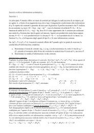
The implications of this hypothesis are illustrated in Fig. 1, 

which shows the change that would occur in production if, from 

an initial equilibrium position, demand were to fall by one unit 

at time zero and to remain constant thereafter, on the assumption 

that the rate of change of production, measured in units per year per 

year, is four times the difference between demand and production,

292 THE ECONOMIC JOURNAL [JUNE 

both measured in units per year. The factor of proportionality, 

4 in this case, is a measure of the speed of response of production 

to changes in demand, and is indicated in Fig. 1 by the slope of 

the line OB, drawn tangential to the production-response curve at 

0. Its reciprocal is a measure of the slowness of response, or time 

taken to adjust production to changes in demand, and is called 

the time constant of the production lag. In this case it is equal 

to 3 months or 025 of a year, and is indicated in Fig. 1 by the 

length of the line AB. The time constant may also be defined 

as the time that would be taken, after a sudden change in demand, 

for production to change by an amount equal to 0632 1 of the 

full adjustment required for a new equilibrium, if demand were 

meanwhile to remain constant at its new value. 

It is possible that a better representation of the real process 

of adjustment would be obtained by analysing the time lag into 

a number of separate components operating consecutively. For 

example, there may be a time lag in observing that an adjustment 

is necessary, another in making the decision to carry out the 

adjustment, and a third in actually making the adjustment. 

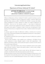
If two such lags are assumed, each with a time constant of 61 

weeks so that the combined time constant is 3 months as in the 

previous example, the time path of the adjustment becomes that 

shown in Curve (b) of Fig. 2, while if three consecutive lags are 

assumed, each with a time constant of 43 weeks, the time path 

becomes that shown in Curve (c) of Fig. 2.2 Although the slower 

adjustment obtained in the initial stages of the process with these 

multiple lags may be more realistic than that which results from 

the assumption of a single lag, the single lag is retained in the 

following analysis in order to simplify the mathematics.3 In all 

the illustrations given below, the time constant of this single 

production lag is assumed to be 3 months. 

In the complete model demand does not remain constant 

during the process of adjustment, but itself responds to changes 

in real income and production. It is therefore necessary to 

1 Or 1 - e1, where e is the base of Napierian logarithms. 

2 If the number of consecutive lags is increased indefinitely, the time constants 

of the separate lags being simultaneously reduced so that the combined time 

constant remains fixed, the time path approaches the limit of a step function, 

jumping from 0 to -1 after a period of time equal to the combined time constant. 

I am indebted to Mr. J. Wise for providing me with a rigorous mathematical 

proof of this. 

3 Since aggregate production includes services, the provision of which responds 

instantaneously to changes in the demand for them, the more rapid initial response 

obtained by assuming a single lag may in fact represent quite a good approxima- 

tion to the real process of adjustment.

1954] STABILISATION POLICY IN A CLOSED ECONOMY 293 

distinguish between an initial or spontaneous change in demand, 

representing a disturbance or change in the relationships of the 

model, and the additional or induced changes in demand which 

result from the dependence of demand on production and in turn 

induce further changes in production by the familiar multiplier 

process. When these induced effects are taken into account the 

-25- 

-.50- 

'-75 

-1 00 

Time in years 

0 *25 50 75 1[00 1 25 1'50 1L75 200 

0- --( 

(c) 

(a) 

(b) 

Production 

Demand 

FIG. 2 

Curve (a), single production lag. 

Curve (b), double production lag. 

Curve (c), triple production lag. 

response of production, measured from a-n initial equilibrium 

value, to a spontaneous fall in demand of one unit, occurring at 

time zero and continuing thereafter, is shown by Curve (a) of Fig. 

3. This is, of course, simply a continuous version of the ordinary 

multiplier process, the multiplier being the reciprocal of the 

marginal leakage, or 4. 

2. The Stabilisation Problem 

The adoption of a policy for stabilising production implies that 

there is some level of production which it is desired to maintain. 

The desired level may be that which, given the existing productive 

resources, would result in a certain level of employment, or it may 

be that which would result in a constant price index of consumers' 

goods, or the choice may be based on a number of other economic, 

political or social considerations. For the limited purpose of 

studying the principles of stabilisation in a closed economy the 

choice of desired production may be considered as given. The 

difference between the actual production and desired production 

at any time will be called the error in production. 

Stabilisation policy consists in detecting any error and taking


correcting action, by altering government expenditure, taxation, 

or monetary and credit conditions, in order to change demand in 

a direction which tends to eliminate the error. The amount by 

which aggregate demand would be changed as a direct result of, 

the stabilisation policy (i.e., excluding the further changes in 

demand which will be induced automatically through the operation- 

of the multiplier process) if the policy were to operate without 

time lag will be called the potential policy demand, and the 

amount by which aggregate demand is in fact changed at any 

time as a direct result of the policy will be called the actual 

policy demand. Both may, of course, be either positive or 

negative. 

The actual policy demand will usually be different from the 

potential policy demand, owing to the time required for observing 

changes in the error, adjusting the correcting action accordingly 

and for the changes in the correcting action to produce their full 

effects. A distributed time lag can again be introduced by the 

hypothesis that whenever such a difference exists the actual 

policy demand will be changing in a direction which tends to 

eliminate the difference and at a rate proportional to the difference. 

The time constant of this lag can then be defined in the same way 

as was done in the case of the production lag. The examples 

given below have been worked out for alternative correction lags 

with time constants of six months and six weeks respectively. 

A number of different types of stabilisation policy will now 

be considered, corresponding to the different ways in which the 

correcting action taken may be related to the error in production.' 

3. Proportional Stabilisation Policy 

The simplest type of stabilisation policy is one in which thIe 

correcting action taken is such that the potential policy demand 

is made proportional in magnitude and opposite in sign 2 to the 

error in production. The ratio of the potential policy demand to 

the error, which is a measure of the strength of the stabilisation 

policy, will be called the proportional correction factor. As an 

example, a proportional correction factor of 0.5 would mean that 

1 The following treatment is an application of the general principles of 

automatic regulating systems and closed-loop control systems, in the analysis of 

which notable advances have been made in recent years. Cf. G. H. Farrington, 

Fundanmentals of Automatic Control, Chapman and Hall, London, 1951; and Brown 

and Campbell, Principles of Servomechanisms, John Wiley and Sons, New York, 

1948. On the use of closed-loop control theory in economics, cf. A. Tustin, The 

Mechanism of Economic Systems, Heinemann, London, 1953. 

2 That is, the principle of " negative feed-back " is used.

19541 STABILISATION POLICY IN A CLOSED ECONOMY 295 

if production was 2% below the desired value the authorities 

cancerned would attempt directly to stimulate demand by an 

amount equal to 1% of production (excluding the further increase 

which would be induced through the multiplier effects), and as 

the error was gradually reduced as a result of this action they 

would decrease the potential policy demand proportionatcly. 

To show the effect of such a policy, it will be assumed that from 

an equilibrium position with production at the desired value 

there occurs at time zero and continues thereafter a spontaneous 

Years 

0 1 2 3 4 5 6 7 8 

(c) 

-1- / (b) 

-2 

-3 

-4 ~~~~~~~~~(a) 

FIG. 3 

Curve (a), no stabilisation policy. 

Curve (b), f,p = 0.5, T = 6 months. 

Curve (c), fp = 2, T = 6 months. 

Note.-The symbols used in Figs. 3 to 9 inclusive have the following meanings: 

P Change in production (measured from initial equilibrium). 

f,p Proportional correction factor. 

fi Integral correction factor. 

fd Derivative correction factor. 

T Time constant of the correction lag. 

fall in demand of one unit. The resulting time path of production, 

if the proportional correction factor is 0-5 and the correction lag 

has a time constant of 6 months, is shown by Curve (b) of Fig. 3. 

The marginal leakage is assumed, as before, to be 025 and the 

production lag to have a time constant of 3 months, so the effect 

of the stabilisation policy can be seen by comparing Curve (b) with 

Curve (a). Curve (c) of Fig. 3 shows the effect of a stronger 

policy with a proportional correction factor of 2, the time constant 

of the correction lag again being 6 months. In the examples 

illustrated in Fig. 4 the time constant of the correction lag has 

been reduced to 6 weeks, the proportional correction factor again 

being zero for Curve (a), 05 for Curve (b) and 2 for Curve (c).


Two defects of a proportional stabilisation policy are im- 

mediately apparent. First, complete correction of an error is 

not obtained, since the correcting action continues only because 

the error exists. If the spontaneous change in demand is denoted 

by 8, the error in the final equilibrium level of production by c, 

the proportional correction factor by fp and the marginal leakage 

by 1, in the final equilibrium the sum of the spontaneous and the 

policy changes in demand will be 8 -f,E. The usual multiplier 

formula applies, so the total change in demand and production, 

Years 

O 1 2 3 4 5 6 7 8 

^ _ _ _ 

_~~~~(C __ 

'-I t_ (b) 

-2 

P\ 

-3 

FIG. 4 

(a) 


Curve (b), fp- = O5, T = 6 weeks. 

Curve (c), fl, = 2, T = 6 weeks. 

including the change induced by the multiplier process, will be 

8 - 

But the change in production is also the error, so that 

_______ E, from which c e = _ + f* When this type of policy is 

applied, therefore, the static multiplier becomes the reciprocal of 

the sum of the marginal leakage and the proportional correction 

factor, and a proportional correction factor of infinity would be 

required if the error were to be completely eliminated. The 

second defect of a proportional stabilisation policy is that it 

tends to cause a cyclical fluctuation in the time path of production, 

this fluctuation being the greater, the stronger the policy and the 

longer the time lag involved in applying it. 

It may be noted that the proportional correction factor and 

the marginal propensity to save, or more generally any marginal 

leakage, have similar effects on the stability of the system. With


a marginal propensity to save of zero, the simple multiplier 

system assumed so far would have no inherent regulation at all, 

i.e., no stable equilibrium position would exist. With a positive 

marginal propensity to save, the change in demand resulting from 

a given change in production would differ from what it would 

have been if the marginal propensity to save had been zero by an 

amount proportional in magnitude and opposite in sign to the 

change in production. The marginal propensity to save therefore 

acts as a regulating mechanism of the proportional type inherent 

in the economy. 

4. Integral Stabilisation Policy 

An integral stabilisation policy is one in which the potential 

policy demand at any time is made proportional in magnitude 

and opposite in sign to the cumulated error up to that time, t.e., 

to the time integral of the error instead of to the magnitude of 

the error. In terms of Figs. 3 and 4, with an integral stabilisation 

policy the potential policy demand at any time is made propor- 

tional to the area between the actual production curve and the 

desired production curve (or zero line) up to that time, whereas 

with a proportional stabilisation policy it is made proportional to 

the vertical distance between the two curves at that time. The 

ratio of the potential policy demand to the time integral of the 

error will be called the integral correction factor. If an error in 

production of 2% -were to occur and to persist for a year, then 

with an integral correction factor of 0 5 the potential policy 

demand would be increased steadily from zero at the beginning 

to 1% of production at the end of the year. It is clear that with 

an integral stabilisation policy the final equilibrium position, if 

it exists, will be one in which the error is completely eliminated, 

since so long as even the smallest error persists the cumulated 

error or time integral of the error must be continuously increasing, 

and with it the magnitude of the correcting action, so that equili- 

brium is possible only when the error is zero. 

It will be found, however, that in thus avoiding the first defect 

of a proportional correction policy, the second defect, the intro- 

duction of cyclical fluctuations, is greatly aggravated, and for 

this reason integral correction is rarely used alone in automatic 

control systems. There may, however, be a tendency for monetary 

authorities, when attempting to correct an " error " in production, 

continuously to strengthen their correcting action the longer the 

error persists, in which case they would be applying an integral 

No. 254.-VOL. LXIV. x

298 THE ECONOMIC JO'URNAL [JUNxE 

correction policy.1 Also, it will be argued in Section II of this 

article that flexible prices in an economy operate as an inherent 

regulating mechanism of the integral type. The integral relation- 

ship may therefore be of some importance in a number of economic 

adjustments. 

-5 

3 

2 

0 

i 2~~ 3 ~~~ 4 6 7 

P~ 

FIG. 5 


Curve (b), fi X05, T _ 6 months. 

Curve (c), f = 2, T = 6 months. 

Figs. 5 and 6 show the effects of applying an integral stabil- 

isation policy. The assumptions of the basic model and the type 

of disturbance are the same as in the previous examples. Curves 

1 International adjustments are not dealt with in this article; but it may be 

worth noting here that a country which attempts to regulate its current balance 

of payments, whether by means of internal credit policy or quantitative import 

control, and in doing so responds mainly to the size of its foreign reserves (i.e., to 

the time integral of its current balance of payments) is applying an integral 

correction policy which is likely to cause cyclical fluctuations similar to those 

illustrated in Figs. 5 and 6. The short cycles which have occurred in the balances 

of payments of a number of countries since the war may be in part the result of 

such action.


(a) again show the response of production to unit spontaneous fall 

in demand when there is no stabilisation policy. In Fig. 5, Curve 

(b) shows the effect of adopting a stabilisation policy with an 

integral correction factor of 0.5, and Curve (c) the effect of a 

stronger policy with an integral correction factor of 2, the time 

constant of the correction lag being 6 months in each case. 

Curves (b) and (c) in Fig. 6 show how the response is modified 

when the time constant of the correction lag is reduced to 6 weeks, 

the integral correction factor again being 0.5 for Curve (b) and 2 

for Curve (c). 

2 

-2 

-3 

0 

-4C 

Years 

1 2 3 4 5 6 7 8 

(a)\ 

(b) 

FIG. 6 


Curve (b), fi = 0-5, T = 6 weeks. 

Curve (c), f- = 2, T = 6 weeks. 

It will be seen that even with a low value of the integral 

correction factor, cyclical fluctuations of considerable magnitude 

are caused by this type of policy, and also that the approach to 

the desired value of production is very slow. Moreover, any 

attempt to speed up the process by adopting a stronger policy is 

likely to do more harm than good by increasing the violence of 

the cyclical fluctuations, particularly when the time lag of the 

correcting action is long. With an integral correction factor of 

2 and a correction lag of 6 months, as illustrated in Curve (c) of 

Fig. 3, the svstem has become dynamically unstable. In such a 

case the oscillations would increase in amplitude until limited by 

non-linearities in the system and would then persist within those 

limits so long as the policy was continued.


5. Proportional Plus Integral Stabilisation Policy 

A combination of proportional and integral stabilisation 

policies gives much better results than either policy alone. This 

can be seen from Figs. 7 and 8, in which Curves (a) again show 

the response of production to unit spontaneous fall in demand 

in the absence of stabilisation policy. Curve (b) of Fig. 7 shows 

how this response is modified if a stabilisation policy is adopted 

having a proportional correction factor of 0.5 plus an integral 

correction factor of 0.5, the time constant of the correction lag 

being 6 months. The proportional element in the policy helps to 

speed up correction and to limit the fluctuations caused by the 

. (e) Years 

2 3 4 5 6 7 8 

0- 

-2. 

-3 

-4 

(a) 

FIG. 7 


Curve (b), fp = 05, f 05, T = 6 months. 

Curve (c), fp = 2, f 2, T 6 months. 

Curve (d), f, 8, f, 8, T 6 months. 

Curve (e),fp =f 8, fi 8, fd = 1, T = 6 months. 

integral policy, while the integral element provides the complete 

correction unobtainable with the proportional policy alone. 

Curve (c) of Fig. 7 shows the response when a stronger policy is 

adopted, keeping the same proportion between the two elements, 

both correction factors being raised to 2, while in Curve (d) they 

are raised to 8, the correction lag remaining at 6 months in each 

case. 

In the examples illustrated in Fig. 8 the time constant of the 

correction lag is reduced to 6 weeks. Curve (b) shows the response 

when both proportional and integral correction factors are 065. 

Comparing this with Curve (b) of Fig. 7, it may appear paradoxical 

that with a shorter correction lag a longer time elapses before


something near full correction is obtained. The reason for this is 

that the more rapid operation of the policy results in a smaller 

error in the early stages of the adjustment, so that the cumulated 

error which forms the basis of the integral element is reduced, so 

reducing the speed of the later stages of the -adjustment, which 

depend mainly on the integral element. The shorter the correction 

lag, therefore, the greater must be the integral correction factor 

if rapid correction is to be obtained. Conversely, of course, the 

longer the correction lag the smaller must be the integral correction 

factor if overshooting and fluctuations are to be avoided. A 

P\ -2 

-3 

-4 

I (f) (e) Years 

/1 2 3 4 5 6 7 8 

0' 

FIG. 8 


Curve (b), fp = 0 5, f = 0 5, T = 6 wdeks. 

Curve (c), fp = 0.5, fi = 2, T = 6 weeks. 

Curve (d), f, = 2, fi = 8, T = 6 weeks. 

Curve (e), fp = 8, fi = 32, T = 6 weeks. 

Curve (f), fp = 8, fi = 32, f = 0-25, T = 6 weeks. 

proportional correction factor of 0.5 plus an integral correction 

factor of 2 gives the response shown by Curve (c) of Fig. 8, while 

for Curve (d) the proportional and integral correction factors are 

2 and 8, and for Curve (e) 8 and 32 respectively. 

The fluctuations in the responses shown in Curves (b), (c) and 

(d) of Fig. 7 and in Curves (c), (d) and (e) of Fig. 8 could be elimin- 

ated by a sufficient reduction in the integral correction factor in 

each case; but only at the cost of increasing both the maximum 

size of the error and the time taken to correct it. A better method 

is available which not only eliminates the fluctuations, but also 

reduces both the maximum size of the error and the time taken 

to obtain complete correction.

302 THE ECONOMIC JOURNAT [JUNE 

6. The Addition of Derivative Correction 

This method is to add to the potential policy demand, as 

determined by the proportional and integral relationships, a 

third element, proportional in magnitude and opposite in sign 

to the rate of change, or time derivative, of production. The 

effect of this is to make demand lower than it would otherwise 

have been whenever production is rising, and higher than it would 

otherwise have been whenever production is falling, so tending to 

check movements in either direction without affecting the final 

equilibrium position. The ratio of the magnitude of this element 

in the potential policy demand to the rate of change of production 

is called the derivative correction factor. 

Curve (e) of Fig. 7 shows the response of production to a unit 

fall in demand when a proportional plus integral plus derivative 

stabilisation policy is applied, the correction factors being 8, 8 

and I respectively, with a correction lag of 6 months. This may 

be compared with Curve (d) of Fig. 7, which shows the response 

when the derivative element of the policy is omitted, the other 

elements being unchanged. Similarly, the addition of a derivative 

element with a correction factor of 0-25 to a proportional plus 

integral policy with correction factors of 8 and 32 respectively 

and a correction lag of 6 weeks modifies the response from that 

shown by Curve (e) of Fig. 8 to that shown by Curve (f). It will be 

noticed that in order to maintain a suitable balance between the 

three elements in the policy when the length of the correction lag 

is reduced, it is necessary to reduce the derivative correction 

factor in about the same proportion as the time constant of the 

correction lag, whereas the integral correction factor had to be 

increased in about the same proportion. 

The reader may have observed that the application of a 

derivative correction policy introduces into the system the same 

type of relationship as that postulated by the acceleration prin- 

ciple, but operating in the opposite direction, the additional 

policy demand being opposite in sign to the rate of change of 

production, whereas the additional investment demand resulting 

from the operation of the acceleration principle is of the same 

sign as the rate of change of production. This means that so far 

as its effect on system stability is concerned, the acceleration 

principle acts as a perverse or destabilising derivative correction 

element. The usefulness of the acceleration hypothesis has some- 

times been questioned. But stated in the moderate form, that 

when production is rising entrepreneurs will want to invest at a


greater rate, and after a time will in fact invest at a greater rate, 

than they would have done if production had not been rising, 

and conversely in the case of falling production, there can hardly 

be any doubt that the principle is a valid one. It seems desirable, 

therefore, to investigate the effects of stabilisation policies when 

the basic multiplier model is modified by the inclusion of an 

acceleration relationship. 

7. Stabilisation of a Multiplier--Accelerator Model 

We may define the term potential acceleration demand as the 

increase in investment demand that would occur as a direct result 

of rising production if the rise were to continue long enough for 

investment demand to become completely adjusted to it (and 

conversely in the case of falling production), and the term ac- 

celeration coefficient as the ratio between the potential acceleration 

demand and the rate of change of production which causes it.' 

Since investment demand will not respond instantaneously to 

alterations in the rate of change of production, a time lag may be 

introduced by the hypothesis that the actual acceleration demand 

tends continuously to approach the potential acceleration demand 

at a rate proportional to the difference between them. The time 

constant of this lag is defined in the same way as in the case of the 

production and correction lags. 

Curve (a) of Fig. 9 (drawn with a different production scale 

from that used in Figs. 3-8 because of the greater fluctuations 

obtained) shows the response of production to unit spontaneous 

fall in demand when there is a marginal leakage of 0-25, a produc- 

tion lag with a time constant of 3 months, an acceleration co- 

efficient of 0*6 and an acceleration lag with a time constant of 1 

year, and when there is no stabilisation policy. With these values 

an explosive cycle is generated,2 the fall in production in the first 

phase of the cycle being about 14 times as great as the spontaneous 

fall in demand. The cycle would eventually be limited by non- 

linearities in the system, and would then persist within those 

limits. 

1 Defined in this way, the acceleration coefficient is also the ratio of the change 

in the desired stock of capital to the change in the annual rate of production and 

real income, or what might be called the marginal desired capital-income ratio. 

2 The system gives damped oscillations when the acceleration coefficient lies 

between 0 and 0 5, explosive oscillations when it lies between 0.5 and 1, and is 

explosive without oscillations when the acceleration coefficient is greater than 1. 

All these values would probably be raised if the production and acceleration lags 

were divided, as they no doubt should be, into a number of separate shorter lags 

(observation lags, decision lags, process lags, etc.), and if similar lags were intro- 

duced in the response of demand to changes in income.

304 THE ECONOMIC JOURNAL [JINE 

The application of a stabilisation policy having a proportional 

correction factor of 2 and a correction lag with a time constant 

of 6 months would change the response to that shown by Curve 

(b) of Fig. 9, and the addition to this policy of an integral element 

with a correction factor of 2 would change the response to that 

shown by Curve (c). As might be expected, the effect of the ac- 

celeration relationship has been to increase both the magnitude 

and the duration of the fluctuations resulting from these policies. 

(These responses may be compared with those shown by Curve 

(c) of Fig. 3 and Curve (c) of Fig. 7.) 

Is 

P 4 

FIG. 9 


Curve (b), fp = 2, T = 6 months. 

Curve (c), fp = 2,fs = 2, T = 6 months. 

Curve (d), fp = 2, = 2, fd O055, T = 6 months. 

Curve (e), f = 8,fs = 8,fd =d 13, T = 6 months. 

To eliminate these fluctuations it would be necessary to add 

a derivative element to stabilisation policy. A derivative correc- 

tion factor of 0-3 would be needed to offset the acceleration 

coefficient of 0-6 (the derivative correction factor need be only 

half the size of the acceleration coefficient in this case, since the 

length of the correction lag is only half that of the acceleration 

lag), and an additional derivative correction factor of 0*25 would 

be needed to eliminate the fluctuations introduced by the propor- 

tional and integral elements of the stabilisation policy. Adding 

therefore a derivative element with a correction factor of 0.55 

the response shown by Curve (d) of Fig. 9 is obtained. Finally, 

if the stabilisation policy was strengthened by multiplying each

1954] STABLISATION POLICY IN A CLOSED ECONOMY 305 

correction factor (excepting that part of the derivative correction 

factor which was needed to offset the acceleration coefficient) by 

four, the response shown by Curve (e) would be obtained. 

These results appear to indicate that if any stabilisation 

policy 1 is to be successful it must be made up of a suitable com- 

bination of proportional, integral and derivative elements. A 

strong proportional element is needed as the main basis of the 

policy, sufficient integral correction should be added to obtain 

complete correction of an error within a reasonable time and an 

element of derivative correction is required to overcome the oscil- 

latory tendencies which may be introduced by the other two 

elements of the policy. If the system itself has a considerable 

tendency to oscillate as a result of a perverse derivative relation- 

ship inherent in it in the form of the acceleration principle, the 

integral element in the policy should be made very weak or 

avoided entirely, unless it can be accompanied by sufficient 

derivative correction to offset the destabilising effects of the 

perverse derivative relationship. 

8. Diagrammatic Representation of the System 

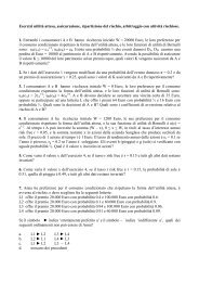
The system of relationships used in this Section can be represented 

by a block diagram of the type frequently employed in 

the analysis of closed-loop systems. In Fig. 10 the lines represent 

variables and the squares represent relationships between 

variables, the particular relationship in each case being indicated 

by the symbol within the square. D indicates differentiation 

with respect to time, f indicates integration with respect to time 

and L indicates the operation of a distributed time lag in the 

adjustment of one- variable to another. Brackets indicate multiplication 

by the parameter inside the brackets. The arrows 

show the direction of causation or the sequence of responses. 

Circles represent addition or subtraction according to the algebraic 

signs shown in each case. 

The simple multiplier model is represented by the single 

closed loop at the bottom of the diagram. Production P is 

related to demand E through the operation of the production 

time lag L., and in turn influences demand through the marginal 

propensity to spend (1 - 1), I being the marginal leakage. The 

1 The general principles of stabilisation have been illustrated here with 

particular reference to aggregate production in a closed economy, but they are 

of quite general applicability. They could equally well be used, for example, in 

investigating the stability of adjustments in international trade, or the problems 

involved in commodity price stabilisation schemes.

306 THE ECONOMIC JOTJZRNAL [JUNE 

loop immediately above this represents the acceleration principle, 

which adds another component to demand equal to the rate 

change of production dt- multiplied by the acceleration coefficiei.t 

k and subject to the acceleration time lag La. 

The three loops at the top of the diagram represent the three 

types of stabilisation policy. The error in production E is 

obtained by subtracting the desired production Pd from the 

actual production. (In the illustrations given in this article all 

variables are measured as deviations from their values in an 

initial equilibriunm position with production at the desired level. 

Pd-~ 

Pt_ 

dP 

D d (k La 

P ++ 

FIG. 10 

+? +E 

Pd is therefore zero and e equals P.) The error, the integral of 

the error and the derivative of the error are multiplied by-fp, 

- fi and - fd respectively, fp. being the proportional correction 

factor, fi the integral correction factor and fd the derivative 

correction factor. The potential policy demand - is the sum of 

these products, and subject to the operation of the correction 

time lag L, determines the actual policy demand which is added 

to the other components of aggregate demand. 

The variable u represents a disturbance to the system, assumed 

throughout this article to take the form of a spontaneous fall in 

demand of one unit at time zero. Other forms of disturbance 

could, of course, be assumed and their effects investigated, and 

disturbances could be applied to other variables instead of, or 

in addition to, demand. 

u 

P 

1p


SECTION II 

A Model with Flexible Prices 

1. The Relationship between Prices and Production 

If changes in the quantity and productivity of the factors of 

production are ignored, the change in the average level of product 

prices which results from a given change in the aggregate level 

of production will be the sum of two components. First, if the 

prices of the services of the factors of production (which will be 

referred to for brevity as factor prices) are absolutely rigid, 

product prices, tending to move with marginal costs, will vary 

directly with the level of production. This component of the 

change in product prices is probably not very large, and will be 

neglected in the following analysis. 

Second, if factor prices have some degree of flexibility, there 

will be changes in product prices resulting from the changes which 

take place in factor prices. Even with flexible factor prices, 

there will be some level of production and employment which, 

given the bargaining powers of the different groups in the economy, 

will just result in the average level of factor prices remaining 

constant, this level of production and employment being lower, 

the stronger and more aggressive the organisation of the factors 

of production. If aggregate real demand is high enough to make 

a higher level of production than this profitable, entrepreneurs 

will be more anxious to obtain (and to retain) the services of 

labour and other factors of production and so less inclined to 

resist demands for higher wages and other factor rewards. Factor 

prices will therefore rise. The level of demand being high, the rising 

costs will be passed on in the form of higher product prices. 

Factor and product prices will continue to rise in this way so long 

as the high level of demand and production is maintained, the 

rate at which they rise being greater, the higher the level of demand 

and production. 

Conversely, if aggregate real demand is so low that production 

at the level which would result in constant factor prices is un- 

profitable, entrepreneurs will be more anxious to force down 

factor prices, while at the lower level of employment factors will 

be less able to press for higher rewards and more inclined to 

accept lower rewards. Factor prices will therefore gradually 

move downwards, and the level of demand being low, the falling 

costs will be reflected in falling product prices. Prices will con- 

tinue to fall in this way so long as demand and production remain

308 TH:E ECONOMIC JOURNAL [JUNE 

low, the rate of fall being greater, the lower the level of demand 

and production. 

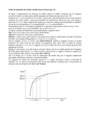
We may therefore postulate a relationship between the level 

of production and the rate of change of factor prices, which is 

probably of the form shown in Fig. 11, the fairly sharp bend in 

the curve where it passes through zero rate of change of prices 

being the result of the greater rigidity of factor prices in the 

downward than in the upward direction. The relationship 

between the level of production and the rate of change of product 

prices will be of a similar shape if productivity is constant. In 

Rate of 

change of 

prices 

FIG. 1 1 

Level of 

production 

spite of the marked curvature of the relationship, linearity may 

be assumed as an approximation for small changes in production. 

If the desired level of production is now taken to be that which 

would result in a constant level of product prices, we may say 

that the rate of change of product prices will be approximately 

proportional to the deviation of production from this level, i.e., 

to the error in production, this approximation being better, the 

smaller the fluctuations which occur in production. 

2. Additional Relationships when Prices and Interest Rates are 

Flexible 

The model used in Section I can now be extended by dropping 

the assumption of constant prices and interest rates. The com- 

plete model is shown diagrammatically in Fig. 12, which is the 

same as Fig. 10 excepting for the addition of the group of relation- 

ships in the centre of the diagram. Four additional sequences 

can be distinguished. 

(i) A deviation of production from the desired level will be 

accompanied by a change in the number of transactions and so 

a change in the amount of money needed for conducting them, 

even if prices are rigid. If the quantity of money is less than 

perfectly elastic, this will cause interest rates, i, to change in the 

same direction 1 as the error in production. As a result of this 

1 Provided that the liquidity preference schedule does not shift.

1954] STABLISATION POLICY IN A CLOSED ECONOMY 309 

change in interest rates there will be a potential change 1 i 

investment demand and production, in the opposite direction 

to the error in production and (assuming linearity throughout) 

proportional to the error. This sequence of responses is repre- 

sented in Fig. 12 by the closed loop of relationships (a), (b), 

Pd- 

+ 

+ 

(>~~-b Ls 

dP 

D dt (k) L_a. 

p ~ 1)+ + 4+ELP 

FIG. 12 

L1, Lp, giving a potential feed-back of - abP and so acting as a 

regulating mechanism of the proportional type. 

(ii) If prices, p, are flexible, the error in production will also 

cause prices to change at a rate proportional to the error. The 

amount by which prices have changed at any given time, being 

identical with the time integral of their rate of change up to that 

time, will be proportional to the time integral of the error. This 

1 It will be remembered that by a potential change in any variable we mean 

the change that would take place if no time lag was involved.


change in prices will cause a further change in the amount of 

money needed for conducting transactions, in addition to that 

caused by the change in the number of transactions conducted. 

There will therefore be an additional change in interest rates 1 in 

the same direction as the error, causing a further potential change 

in investment demand and production in the opposite direction 

to the error and proportional to the time integral of the error. 

This sequence of responses thus operates as a regulating mechanism 

of the integral type. The sequence is represented in Fig. 12 by 

the relationships (c), f, (h), ( b), L1, Lp, which give a potential 

feed-back of - chbfP. 

(iii) Professor Pigou has pointed out2 that even if the liquidity 

preference schedule was infinitely elastic at the prevailing level 

of interest rates, so that interest rates failed to move with a 

change in production and prices, a change in the level of prices 

would still influence demand by changing the real value of money 

balances and so the amount of saving at given incomes and interest 

rates. This potential change in demand would be in the same 

direction as the change in the real value of money balances, and 

therefore in the opposite direction to the change in prices. For 

small changes it would be approximately proportional to the 

change in prices and therefore proportional to the time integral 

of the error in production. The Pigou effect is therefore equivalent 

to another integral regulating mechanism inherent in the economy. 

It is represented in Fig. 12 by the closed loop of relationships 

(c), , (- n), L2, Lp, giving a potential feed-back of - cmfP. 

I The device of considering the quantity effects and price effects separately 

and then adding them can be justified as follows: Denoting interest rates, 

production and prices, measured from a zero base, by i0, PO and po respectively, 

and deviations from their initial equilibrium values by i, P and p, we have 

to = F(PO, Po) 

Expanding this expression in a Taylor series and dropping all but the first two 

terms gives 

or 

aio -- Aap az' o + apo APO 

+ .- 

at ai 

as an approximation valid for small changes. For small changes V. and V- may 

also be considered constant, so we may write 

i = aP + hp 

which is the relationship shown in Fig. 12. Similar approximations are involved 

in considering the change in aggregate demand as the sum of a number of separate 

components. 

2 " The Classical Stationary State," EcoNoMIc JoURNAL, December 1943, 

and " Economic Progress in a Stable Environment," Economica, August 1947.

1954] STABILISATION POLICY IN A CLOSED ECONOM Y 311 

(iv) Demand is also likely to be influenced by the rate at 

which prices are changing, oi have been changing in the recent 

past, as distinct from the amount by which they have changed, 

this influence on demand being greater, the greater the rate of 

change of prices. Since the rate of change of prices in turn depends 

on the error in production, the potential change in demand and 

production resulting from these relationships will be approximately 

proportional to the error in production. This sequence of re- 

sponses is represented in Fig. 12 by the relationships (c), (n), L3, 

Lp, the potential feed-back therefore being cnP. The direction 

of this change in demand will depend on expectations about 

future price changes. If changing prices induce expectations of 

further changes in the same direction, as will probably be the case 

after fairly rapid and prolonged movements, demand will change 

in the same direction as the changing prices. That is, n will be 

positive, and there will be a positive feed-back tending to intensify 

the error, the response of demand to changing prices thus acting 

as a perverse or destabilising mechanism of the proportional type. 

If, on the other hand, there is confidence that any movement of 

prices away from the level ruling in the recent past will soon be 

reversed, demand is likely to change in the opposite direction 

to the changing prices. n will then be negative, and the response 

of demand to changing prices will act as a normal proportional 

regulating mechanism. 

3. Inherent Regulation of the System 

Some examples will be given below to illustrate the stability 

of this system under different conditions of price flexibility and 

with different expectations concerning future price changes. As 

before, it will be assumed that the marginal leakage is 0-25 and 

that the time constant of the production lag is 3 months. The 

time constants of the lags L1, L2 and L3 will be taken as 6 months. 

The acceleration relationship will be omitted (by putting k _ 0) 

so that the effects of price flexibility can be seen by comparing 

the response of the system with that of the multiplier model. 

In deciding upon suitable values for the remaining parameters 

it will be convenient to think of the units being such that in the 

initial equilibrium position production is 100 units per year, the 

price index also being 100. Changes can be expressed in either 

absolute or percentage terms with negligible error so long as 

prices and production do not move too far from their initial 

equilibrium values. The product of the parameters a and b will be 

given the value 0-2, which is equivalent to assuming that if

312 THE ECONOMIC J,OuIRNAL [JUNE 

production were to fall by 1% or 1 unit, prices remaining constant, 

interest rates would fall sufficiently to stimulate investment 

demand by 0-2 of a unit. The product of the parameters h and b 

must be a little greater than this, since if the price level were to 

fall by 1%, production remaining constant, there would be the 

4 

3(d 

2 

(c) 

~~Years 

_12 

0 

3 4 6 7 

P (e) (b) 

-3 

-4 

-2 ~~Cre c,c=1,n=02 

-5 

-6 

(a) 

FIG. 13 

Curve (a), zero price flexibility (o 0). 

Curve (b), c = 05, n = 0-2. 

Curve (c), c =1, n = 0*2. 

Curve (di), c = 2, n = 0*2. 

Curve (e), with stabilisation policy. 

same reduction in the demand for money for transactions pur- 

poses; but the real value of money balances would be slightly 

increased so that the fall in interest rates would be rather greater. 

The product hb will therefore be given the value 0-25. m will be 

taken as 0 05, equivalent to assuming that a 1% fall in the price 

level would stimulate demand by 0.05% through its effect in

1954] STABILISATION POLICY IN, A CLOSED ECONOMY 313 

increasing the real value of money balances, if there was no 

change in interest rates. 

The responses shown in Fig. 13 have been worked out on the 

assumption that n has the value 0-2. This means, for example, 

that if prices are falling at the rate of 1% per-year, demand will 

tend to be 0-2 of 1% lower that it would have been if prices had 

been constant. Given these assumptions, Curve (a) shows the 

response of production to unit fall in demand when there is zero 

price flexibility (c - 0). This response is similar to that of the 

multiplier model (Curves (a) of Fig. 3-8); but the final error is 

less owing to the stabilising effects of the flexible interest rates. 

Curve (b) shows the response when c = 0.5, i.e., when for 

each 1% error in production prices change at the rate of 056% 

per year. The two integral regulating mechanisms now come 

into play, operating through interest rates and the Pigou effect 

respectively, so in the final equilibrium position the error is 

completely corrected. The total strength of the proportional 

regulating mechanisms is, however, reduced by the perverse 

effect of the response of demand to changing prices, with the 

result that the magnitude of the error in the early stages of the 

adjustment is slightly greater than in the case of zero price 

flexibility. 

When c = 1 the response is that shown by Curve (c) and when 

c = 2 it becomes that shown by Curve (d). The strength of the 

integral regulating mechanisms increases with the increasing 

degree of price flexibility, while the total strength of the propor- 

tional regulating mechanisms decreases as demand responds 

perversely to the more rapid rate of change of prices, and both 

these effects tend to introduce fluctuations when price flexibility 

is increased beyond a certain point. When price expectations 

operate in this way, therefore, the system has fairly satisfactory 

self-regulating properties when prices are moderately flexible; 

but becomes unstable when there is a high degree of price 

flexibility. 

If changing prices induce expectations of future changes in 

the reverse direction, n being given the value - 0-2, the response 

of the system when there are different degrees of price flexibility is 

as shown in Fig. 14. Curves (a), (b), (c) and (d) have been worked 

out for values of c of 0, 0.5, 1 and 2 respectively, and so can be 

compared with the- equivalent curves in Fig. 13. In this case 

the response of demand to changing prices provides a normal 

proportional regulating mechanism which increases in strength 

with the increasing degree of price flexibility. This increasing 

No. 254.-VOL. LXIV. y

314 TIHE ECONOMIC JOURNAL [JUNE 

proportional regulation limits the fluctuations which would other- 

wise be introduced as a result of integral mechanisms, the strength 

of which also increases with increasing price flexibility, and at the 

same time increases the speed with which the error is corrected in 

the early stages of the adjustment. We may conclude that the 

self-regulating properties of the system will be considerably 

p 

-2 

-3 

0'I 

Years 

I 2 3 4 5 6 7 8 

d (c) 

(a) 

FIG. 14 

Curve (a), zero price flexibility (c = 0). 

Curve (b), c = 0-5, n = -0-2. 

Curve (c), c = 1, n = -02. 

Curve (d), c = 2, n 0-02. 

improved if there is confidence that any movement of prices away 

from the level ruling in the recent past will soon be reversed, and 

that if such confidence is sufficiently great the self-regulating 

properties will also be better, the higher the degree of price 

flexibility in the system. 

4. Stabtilisation of the System 

If a stabilisation policy is applied to the system, the values of 

the correction factors required to produce any particular response 

will depend on the values of the parameters in the system. 

Examples of the values of correction factors which would result 

in the response shown by Curve (e) of Fig. 13 if the time constant 

of the correction lag was 6 months are given in the following 

table. 

Proposals have sometimes been made for improving the 

stability of the economic system by " building in " additional 

regulating mechanisms. In the British Government's White 

Paper on Employment Policy 1 reference is made to a scheme for 

influencing consumption spending by varying the rates of social- 

insurance contributions above or below the standard rates by 

1 Cmd. 6527, 1944, paragraphs 68-71 and Appendix II.


Stabilisation policy required to produce 

the response shown by Curve (e) of Fig. 13. 

Response of unstabilised 

system. Proportional Integral Derivative 

correction 

factor. 

correction 

factor. 

correction 

factor. 

Curve (a), Fig. 13 1-8 2-0 0-2 

Curve (b), Fig. 13 .19 1F85 0-2 

Curve (c), Fig. 13 2-0 1-7 0-2 

Curve (d), Fig. 13 2-2 1-4 0-2 

Curve (b), Fig. 14 . 1-7 1-85 0-2 

Curve (c), Fig. 14 1-6 1-7 0-2 

Curve (d), Fig. 14 . . 14 14 0-2 

Curve (a), Figs. 3-8 2-0 2-0 0-2 

Curve (a), Fig. 9 2-0 2-0 0-5 

amounts depending on the percentage by which the actual 

employment is above or below the average percentage over a 

period of years. On the basis of the figures given in the White 

Paper to illustrate how the scheme might operate, this would 

introduce a proportional regulating mechanism with a correction 

factor of about 0.2.1 If schemes of this sort could be administered 

successfully they would undoubtedly improve the stability of the 

system considerably, and would probably be more effective than 

attempts to forecast conditions a year or more ahead and adjust 

an annual budget accordingly. 

Monetary policy would be a more convenient instrument for 

stabilising an economy. Some may doubt whether it is a suffi- 

ciently powerful instrument; but if the right type of stabilisation 

policy is being applied continuously, comparatively small cor- 

recting forces are sufficient to hold the system near the desired 

position once that position has been attained. It is quite likely, 

therefore, that a monetary policy based on the principles of 

automatic regulating systems would be adequate to deal with all 

but the most severe disturbances to the economic system. 

1 Professor Meade has suggested a scheme, operating through special monthly 

taxes and credits related to the level of employment, which would have similar 

effects. With the scales of taxes and credits suggested by him the proportional 

correction factor would be about 0 4. The cumulative expansion and con- 

traction of the quantity of money resulting from the proposed method of financing 

the scheme would also introduce an integral correction element. Professor 

Meade must have been aware that there would be some disadvantage in having 

too much integral correction, since he recommended that this effect should be 

partially offset through appropriate action by the central bank. Cf. J. E. 

Meade, Con8umers' Credits and Unemployment, Oxford University Press, London, 

1938.


Mathematical Appendix 

1. Symbols Used 

P aggregate production, in units per year, measured from 

the initial equilibrium value. 

E aggregate demand, in units per year, measured from the 

initial equilibrium value. 

oc the speed of response of production to changes in demand. 

The time constant of the production lag is I years. 

D the differential operator d 

dt' 

t time in years. 

I the marginal leakage. 

u unit step function, equal to zero when t < 0 and to unity 

when t > 0. 

3 the speed of response of policy demand to changes in 

potential policy demand. The time constant of the 

correction lag is f years. 

fp proportional correction factor. 

fi integral correction factor. 

fd derivative correction factor. 

k acceleration coefficient. 

K speed of response of demand to changes in the rate of 

change of production. The time constant of the 

acceleration lag is 1 years. 

If the rate of interest is denoted by i, the price level by p, and 

potential demand by E', the parameters of the price relationships 

shown in Fig. 12 are defined as: 

ai 

a-p ba. 

aE' a(dt) 

ap 

ai 

ap 

aE' 

h- rm=-an ap 

aE' 

a dpA 

2. Distributed Time Lays 

A single distributed time lag in the response of production to 

changes in demand is represented by the equation 

from which 

DP=- (P-E) . (1) 

P . D + a (2)


Similarly, the value of any variable which responds with a 

distributed time lag to changes in another is obtained by multi- 

plying the value which that variable would have if there were no 

time lag by an operator of the form D + where - is the time 

constant of the lag. This rule will be used whenever a time lag is 

introduced. 

If, from equilibrium, demand were to fall by one unit at time 

t = 0, we may substitute E = - P when t > 0, giving 

with the initial condition 

(D + a)P- oc when t > O (3) 

P = O whentO . (4) 

since immediately after the change production will still be at its 

initial value. 

The solution 1 of equations (3) and (4) is 

P - (1 - e-t) 

which is plotted in Fig. 1 and Curve (a) of Fig. 2 for a = 4. 

If there were two consecutive time lags in the response of 

production to demand, the time constant of each being 8 year, 

equation (2) would become 

After the unit fall in demand, this gives 

with initial conditions 

The solution is 

( D + 8) * (2a) 

(D + 8)2P--82whent>O > . 

. (3a) 

P=0,1 DP =O whentO . . (4a) 

P- [1- (1 + 8t)e-8t] 

which is plotted as Curve (b) of Fig. 2. 

With three consecutive time lags each having a time constant 

1 For methods of solving ordinary linear differential equations with constant 

coefficients see Piaggio, Differential Equations, G. Bell & Sons, Ltd., London, 

1949, Chapter 3. For equations of order higher than the second a considerable 

saving of labour is obtained by using the Laplace Transformation instead of the 

classical methods of solution. See Carslaw and Jaeger, Operational Methods in 

Applied Mathematics, Oxford University Press, Oxford, 1948, and Gardner and 

Barnes, Transients in Linear Systems, John Wiley & Sons, New York, 1942.


of 1-- year the equations for the response to unit fall in demand 

would be 

(D + 12)3P --123 whent>0 . . (3b) 

The solution is 

P=0,DP=O,D2P-Owhent=0. . (4b) 

P -[1 - (1 + 12t + 72t2)e12t] 

which is plotted as Curve (c) of Fig. 2. 

3. The Multiplier Model 

The response of demand to changes in production or real 

inconme is represented by the equation 

E = (1- I)P-u . . . . (5) 

u being the spontaneous change in demand occurring at time 

t = 0. Substituting equation (5) in equation (1) and rearranging, 

we obtain 

(D + cl)P - CU. (6) 

After the initial change in demand this becomes 

with the initial condition 

(D + c)P = - cwhen t > 0 (7) 

P=Owhent=O. (8) 

since immediately after the change production will still be at its 

initial equilibrium value. 

The solution of equations (7) and (8) for o = 4 and I- 0-25 is 

p = - 4(1 - et) 

which is plotted as Curves (a) of Figs. 3-9 inclusive. 

4. Proportional Stabilisation Policy 

The potential policy demand is - fpP, giving an actual policy 

demand of - P' P. Adding this to the demand shown in 

equation (5) we obtain 

X = (1 -I)P - PfP P P-q u . (5a) 

Substituting this expression in equation (1) and rearranging gives 

[D2 + (cX + P)D + xt(l +fp)]P = (- ocD - cx3)u (6a)


After the initial change in demand u equals unity and the 

derivatives of u are zero, so that 

[D2 + (Lxl + t)D + oc(l + fp)]P oc= when t > 0 (7a) 

the initial conditions being 

P _ O, DP -oc when t = O (8a) 

The solutions of equations (7a) and (8a) for different values of 

fp and ,B, a and I having the same values as before, are given in 

the following table: 

f. /3. P. Curve. 

065 2 - 1-33- 169e-1 5t sin (1110 t - 52?) Fig. 3 (b) 

2 2 - 044 - 95e- "I" sin (2270 t - 280) Fig. 3 (c) 

0.5 8 - 1*33- 169e-4 5t sin (1110 t - 1280) Fig. 4 (b) 

2 8 - 044 -052e-4 5t sin (4120 t - 58?) Fig. 4 (c) 

5. Integral Stabili,sation'Policy 

With an integral stabilisation policy the actual policy demand 

is - D f fPdt. Adding this to equation (5), differentiating 

with respect to time, then substituting in equation (1) and re- 

arranging the terms, we obtain 

[D3 + (oal + 3)D2 + aclD + cP3fj]P (-acD2 - acD)u (6b) 

After the initial change in demand this becomes 

[D3 + (cl + P)D2 + oc4ID + c43fi]P = O when t > 0 . (7b) 

with initial conditions 1 

P 0, DP= - oc, D2P cx21 = when t == O . (8b) 

1 The initial conditions are not intuitively obvious when the equations are of 

the third or higher order. The following rules, derived from A. Porter, An 

Introduction to Servomechanisms, Methuen & Co., Ltd., London, 1950, pp. 50-3, 

to which the reader is referred for their justification, lay down a simple procedure 

for finding the initial conditions of the system in these cases. 

(i) Integrate the equation with respect to time between the limits t= -0 

and t = + 0. Terms containing integrals of P and u between these limits are 

equal to zero and may be omitted. 

(ii) Repeat the integrations until only the term in P remains. This gives the 

value of P when t = 0. 

(iii) Substitute this value of P in the preceding equation, setting u equal to 

1 and any derivatives of u equal to zero. This gives the value of DP when 

t = 0. 

(iv) Repeat the substitutions until all the initial conditions have been 

obtained.

320 THE ECONOMIC JOURNAIL [JUNE 

The solutions of equations (7b) and (8b) for different values of 

fi and P are given in the table below: 

fi. /. P. Curve. 

0 5 2 0-37e-2 80 - 255e-0?t sin (68.30 t + 8.30) Fig. 5 (b) 

2 

0 5 

2 

2 

8 

8 

0.33e-3 

0 02e-8 

0 04e-8 

65t - 

27 - 

91 - 

1.34e?'33' sin (1180 t + 140) 

2 88e0-037t sin (77.00 t + 0 340) 

135e-0?05t sin (1540 t + 1.80) 

Fig. 5 (c) 

Fig. 6 (b) 

Fig. 6 (c) 

6. Proportional plus Integral Stabilisation Policy 

The actual policy demand in this case is -D 

(fPp +fPdt). 

Following the same procedure as in the previous example, we 

obtain the equations 

[D3 + (cl + r)D2 + ac4(I +fp)D + c43fi]P - 0 when t > 0 (7c) 

P-O, DP - c, D2P _ C21 when t =O (8c) 

Solutions for different values of fp, fi and P are: 

fl,. fi. fd. P. Curve. 

0 5 0 5 2 -133e - 2 67e,t sin (99.40 t - 300) Fig. 7 (b) 

2 2 2 -027et - 1.07e,t sin (2210 t - 15?) Fig. 7 (c) 

8 8 2 -0-06et-' -051e-t sin (4550 t - 70) Fig. 7 (d) 

0 5 0 5 8 -311e-' + (3-11 + 5-33t)e-4t Fig. 8 (b) 

0 5 2 8 -0.11e686t - 1.62e-1,07t sin (1640 t - 4) Fig. 8 (c) 

2 8 8 -022e 4,93t - 0.70e2 03t sin (396? t - 180) Fig. 8 (d) 

8 32 8 -006e-42t - 027e-2 4' sin (8800 t - 130) Fig. 8 (e) 

7. Proportional plus Integral plus Derivative Stabilisation Policy 

The actual policy demand becomes 

- (fp ~-fi Pdt 4fdD)P 

D + p 

Applying these rules to equation (7b) we obtain: 

1st integration D2P + (ol + P)DP + ocplP = ocDu - oc;u (a) 

2nd integration DP + (al + fi)P = cu . . . (b) 

3rd integration P = 0 . . . (c) 

Substituting equation (e) in (b) and setting u equal to unity, 

DP = - c .. (d) 

Substitutilng (e) and (d) in (a) and setting u equal to unity and Du equal to zero, 

D2P - oc(oa + P) = - OCJ 

or D2P= oc21 . .(e) 

Equations (c), (d) and (e) give the initial conditions of the system.


Following the same procedure as before we obtain the equations 

[D3 + (ad + 3 + c4fd)D2 + oc((l +fr)D + cxfi]P = 0 

when t > 0 (7d) 

P = O, DP - - c, D2P - C2(l + 3fd) when t = O (8d) 

Solutions for various values of fv, fi, fd and f3 are: 

fl- fi. fd. f P. Curve. 

8 8 1 2 - 008e-118 -0-68$04 91t sin (3150 t - 60) Fig. 7 (e) 

8 32 025 8 - 007e 5 03t - 031e 5 99t sin (7410 t - 130) Fig. 8 (f) 

8. The Multiplier-Accelerator Model 

The acceleration demand is Kt DP. Adding this to the 

demand shown in equation (5) and following the usual procedure, 

the equations of the system are found to be 

[D2+ (aO + K - OCKk)D + OCKI]P -cK when t > ? (7e) 

P = O, DP =-a when t = 0 (8e) 

With a = 4, 1 = 0.25, K = 1 and k -= 0-6 the solution, plotted as 

Curve (a) of Fig. 9, is 

P = - 4-00 - 6-32 e0,2t sin (560 t - 390) 

When a proportional stabilisation policy is applied the 

equations become 

[D3 + (oca + P + K - OCKk)D2 + (acl + OCKl + 

- OC4Kk)D + 0CfK(l + fp)]P 

PK + OaCfp 

= - OC- K when t > 0 (7f) 

P - 0, DP- -c D2P =a2(l -Kk) when t = O (8f) 

With fv = 2, P - 2 and the other parameters retaining their 

previous values the solution, plotted as Curve (b) of Fig. 9, is 

P = - 0-44 - 0-025 e-1-15t - 1.10 e-0225' sin (2270 t - 250) 

With a proportional plus integral stabilisation policy the 

equations of the system are 

[D4 + (ad + f + K - XKk)D3 + (aOf+l + CKl + PK + Maff 

- CKk)D2 + (a4Kl + C4Kfp + oc4fi)D + G(FKfi]P - 0 

when t > 0 (7g) 

P = (ff + K2Jc) - o 2(l - K k)2 when t = 0 (8g)


With fi = 2, the other parameters retaining their previous values, 

the solution, plotted as Curve (c) of Fig. 9, is 

P - 007 e-143t -013 -069t - 1.08 6026t sin (2310 t - 11?) 

When a proportional plus integral plus derivative stabilisation 

policy is applied the equations of the system become 

[D4 + (Oc + 3 + K + aC(fd - OCKk)D3 + (oc(1 + OCKd + ?K 

+ c4fp + 43IKfd - GC3Kk)D2 + (GCPK1 + C4Kfp + oc4fi)D 

+ ocKfj]P O when t > O (7h) 

P - 0 DP - oc, D2P oc2(1 + rfd - Kk) 

D3P oc2(f + K2k - p2fd) - C3(12 

+ K2k2 + 2 fdl + 32fd2 - 2fKfdk) j 

2Kkl when 

t 0 (8h) 

With fd =/0 55, the other parameters retaining their previous 

values, the solution, plotted as Curve (d) of Fig. 9, is 

p -0.11 e-0 74t + 0.07 e-2 17t - 140 e- 155t sin (1580 t - 20) 

With fp- = 8, fi = 8, fd = 1X3 and the other parameters as before, 

the solution, plotted as Curve (e) of Fig. 9, is 

P = - 0.02 e-0 87t -0-04 e-1 44t - 073 e-0 48t sin (3000 t - 50) 

9. The Model with Flexible Prices and Interest Rates 

If the time constants of the lags L1, L2 and L3 in Fig. 12 are 

assumed for simplicity to be the same as the time constant of the 

correction lag, the total demand resulting from the system 

(excluding the acceleration relationship) is 

E = (1 I)P - ? [(ab - cn + fv)P + (cm + chb 

+ fi)fPdt + fdDP] - u 

Substituting this expression in equation (1) and carrying out the 

same operations as in previous examples, we obtain the following 

equations of the system: 

[D3 + (oc + ! + c'3fd)D2 + oc(l + ab -cn +fp)D 

+ o3(cm + chb +fi)]P = 0 when t > 0 (7i) 

P O, DP - o)D2P = C2(1 ? + fd) when t 0 (8i)


With oc = 4, 1 -025, C = 2, m = 005, ab = 02, hb - 025 

and fp, fi and fd equal to zero, the solutions for various values of 

c and n are shown in the table below: 

c. n. P. Curve. 

0 - - 2-22 - 2.30e1 5t sin (66.50 t - 75.50) Figs. 13 and 

14 (a) 

0 5 

1 

2 

0-2 

0-2 

0-2 

- 0-38e-183t - 800e0-059t sin (32.00 t - 272?) 

0-36e 2 59t - 3-36e-0o21t sin (53.90 t + 6-10) 

0.39e3 32t - 225e?16t sin (68.30 t + 10.00) 

Fig. 13 (b) 

Fig. 13 (c) 

Fig. 13 (d) 

0 5 

1 

2 

- 

- 

- 

0-2 

0-2 

0-2 

- 

- 

- 

2.46e-034t 

2.11e-066t 

1-05e' - 

- 27e-1 33t sin (75.20 t - 64.00) 

- 286e-1,171 sin (86.60 t - 47.60) 

2.31e-t sin (1120 t - 27.20) 

Fig. 14 (b) 

Fig. 14 (c) 

Fig. 14 (d) 

If for each set of values of c and n in the above table, fp, fi 

and fd are given the corresponding values shown in the table on 

page 315, the solution of the system becomes 

P _ - 026 e1141 - 1.10 e-1,73t sin (2070 t - 1361), 

which is plotted as Curve (e) of Fig. 13. 

London School of Economics. 

A. W. PHILLIPS

Stabilisation Policy in a Closed Economy Author(s): A. W. Phillips ...

Create successful ePaper yourself

Delete template?

Save as template?