Stabilisation Policy in a Closed Economy Author(s): A. W. Phillips ...

300 THE ECONOMIC JOURNAL [JUNE
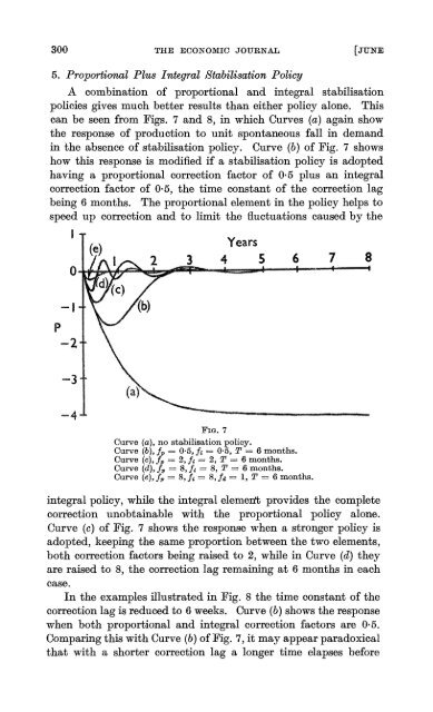
5. Proportional Plus Integral Stabilisation Policy
A combination of proportional and integral stabilisation
policies gives much better results than either policy alone. This
can be seen from Figs. 7 and 8, in which Curves (a) again show
the response of production to unit spontaneous fall in demand
in the absence of stabilisation policy. Curve (b) of Fig. 7 shows
how this response is modified if a stabilisation policy is adopted
having a proportional correction factor of 0.5 plus an integral
correction factor of 0.5, the time constant of the correction lag
being 6 months. The proportional element in the policy helps to
speed up correction and to limit the fluctuations caused by the
. (e) Years
2 3 4 5 6 7 8
0-
-2.
-3
-4
(a)
FIG. 7
Curve (a), no stabilisation policy.
Curve (b), fp = 05, f 05, T = 6 months.
Curve (c), fp = 2, f 2, T 6 months.
Curve (d), f, 8, f, 8, T 6 months.
Curve (e),fp =f 8, fi 8, fd = 1, T = 6 months.
integral policy, while the integral element provides the complete
correction unobtainable with the proportional policy alone.
Curve (c) of Fig. 7 shows the response when a stronger policy is
adopted, keeping the same proportion between the two elements,
both correction factors being raised to 2, while in Curve (d) they
are raised to 8, the correction lag remaining at 6 months in each
case.
In the examples illustrated in Fig. 8 the time constant of the
correction lag is reduced to 6 weeks. Curve (b) shows the response
when both proportional and integral correction factors are 065.
Comparing this with Curve (b) of Fig. 7, it may appear paradoxical
that with a shorter correction lag a longer time elapses before