A SAS® Macro to Compute Added Predictive Ability of New Markers ...

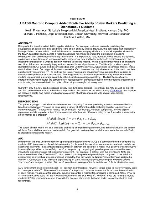
Paper SDA-07
A SAS® Macro to Compute Added Predictive Ability of New Markers Predicting a
Dichotomous Outcome
Kevin F Kennedy, St. Luke’s Hospital-Mid America Heart Institute, Kansas City, MO
Michael J Pencina, Dept. of Biostatistics, Boston University, Harvard Clinical Research
Institute, Boston, MA
ABSTRACT
Risk prediction is an important field in applied statistics. For example, in clinical research, predicting the
development of adverse medical conditions is the object of many studies. However, this concept is multi-disciplinary.
Many published models exist to predict dichotomous outcomes, ranging widely from a model to predict winners in
the NCAA basketball tournament to a recently published risk model to predict the likelihood of a bleeding
complication after percutaneous coronary intervention. It is important to note, however, these models are dynamic,
as changes in population and technology lead to discovery of new and better methods to predict outcomes. An
important consideration is when to add new markers to existing models. While a significant p-value is an important
condition, it does not necessarily imply an improvement in model performance. Traditionally, receiver operating
characteristic (ROC) curves and its corresponding area under the curve (AUC) are used to compare models, with a
statistical test due to DeLong et al. for two correlated AUCs. However, the clinical relevance of this metric has been
questioned by researchers 1,2,3 . To address this issue, Pencina and D’Agostino 1 have proposed two statistics to
evaluate the significance of novel markers. The Integrated Discrimination Improvement (IDI) measures the new
model’s improvement in average sensitivity without sacrificing average specificity. The Net Reclassification
Improvement (NRI) measures the correctness of reclassification of subjects based on their predicted probabilities of
events using the new model with the option of imposing meaningful risk categories.
Currently, only the AUC can be obtained directly from SAS (proc logistic). In contrast, the AUC as well as the NRI
and IDI, can both be outputted in R with the ImproveProb function under the Hmisc library (Click Here). In this paper
we present a single SAS macro which allows calculation of all three measures with several user-defined
specifications.
INTRODUCTION
This paper is going to cover situations where we are comparing 2 models predicting a yes/no outcome without a
time-to-event element. This can be done using a variety of different models, including; logistic, log-binomial, or
Modified Poisson 6,12 approach for relative risk estimation. For example, consider comparing 2 nested logistic
regression models to predict a dichotomous outcome with the main difference being model 2 includes a variable for
a new marker as a predictor:
Model1
: logit(
y)
= α + β x + ... + β x
Model2
: logit(
y)
= α + β x + ... + β x + β
1 1 n n n+
1 n+
1
The output of each model will be a predicted probability of experiencing an event, and each individual in the dataset
will have 2 probabilities, one from each model. Our goal is to evaluate how much the new variables to model2 add
to prediction compared to model1.
AUC
Difference in the area under the receiver operating characteristic curve (AUC) is a common method to compare two
models. AUC is a measure of model discrimination (i.e. how well the model separates subjects who did and did not
experience an event). It essentially depicts a tradeoff between the benefit of a model (true positive or sensitivity) vs.
its costs (false positive or 1-specificity). AUC is computed by comparing all possible pairs in a dataset between
individuals experiencing and not experiencing an event. For example, a dataset with 100 events and 1000 nonevents
would have 100*1000=100,000 pairs. In each pair the predicted probability is compared. If the individual
experiencing an event has a higher predicted probability, that pair would be labeled ‘concordant’ and assigned a
value of 1. Conversely, if the individual experiencing an event has a lower probability the pair would be labeled
‘discordant’ and assigned a value of 0. AUC would be an average of the 1s and 0s (and 0.5s for identical values).
AUC ranges from 0.5 (no discrimination) to 1 (perfect discrimination); however, values close to 1 are very rarely seen
in contemporary data 3,7 . The value of baseline AUC is important, but in our context the focus is on the contribution
of anew marker. To address this scenario, DeLong 4 presented a method for comparing 2 correlated AUCs. Prior to
SAS version 9.2 you could run the %roc macro located on the SAS website 8 . However, if you are running a logistic
model in 9.2 this comparison can be done with the two new statements that were added to proc logistic (roc and
roccontrast).
1
1
1
n
n
x

Sample code for SAS 9.2 Proc Logistic:
proc logistic data=auc;
model eve=x1 x2 x3 x4 x5;
roc 'first' x1 x2 x3 x4;
roc 'second' x1 x2 x3 x4 x5;
roccontrast reference('first')/estimate;
run;
The above code will return a comparison of model 1 (with the first 4 covariates) with model 2 (containing the
additional covariate). For a pre-version 9.2 example go to the SAS website [Click Here].
Many advantages exist for reporting the AUC. First, it is a well known statistic, commonly seen in any model
predicting a dichotomous outcome. Second, it is the default output in most all statistical software including proc
logistic in SAS. Third, there are recommend ranges for an excellent/good/poor value for AUC making it easier to
evaluate the model. In their textbook, Hosmer and Lemeshow 7 consider AUC values of 0.7 to 0.8 to show
acceptable discrimination, values of 0.8 to 0.9 to indicate excellent discrimination, and values of 0.9 to show
outstanding discrimination. However, they also note how unusual it is to observe AUC values over .9 and how it
could cause issues in the model due to complete separation of data.
There are also disadvantages to the AUC. First, it is a rank based statistic. A pair of individuals with probabilities
0.5 and 0.51 would be treated the same as with probabilities 0.1 and 0.9. Second, it focuses only on discrimination
which is not the only and may not be the most important in the context of risk prediction. Third, it is very difficult for a
new marker to significantly change the value of AUC 3 . Fourth, the magnitude of improvement in AUC is not nearly
as meaningful as the value of AUC itself. For this reason it is very difficult to use increase in the AUC to justify
adding new markers to a model even though these markers may have a major impact at the individual level 3 .
The next two measures (IDI/NRI) attempt to quantify the added predictive ability of a new marker by contributing
additional information beyond the AUC. IDI attempts to add to AUC by quantifying how far apart in probabilities the
events and non-events are when adding a new marker. And NRI attempts to quantify how many individuals are
correctly “reclassified” when adding a new marker.
IDI
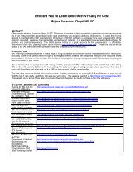
IDI is a measure of the new model’s improvement in average sensitivity (true positive rate) without sacrificing its
average specificity (true negative rate). In comparing the models, IDI measures the increment in the predicted
probabilities for the subset experiencing an event and the decrement for the subset not experiencing an event (see
figure1). This adds an important element that AUC lacks. The AUC is a rank based statistic in which all that matters
is which probability is higher or lower, whereas IDI gives a measure of how far apart on average they are.
Absolute _ IDI = ( p _ event _ 2 − p _ event _1)
+ ( p _ nonevent _1
− p _ nonevent _ 2)
(1)
p _ event _ 2 − p _ nonevent _ 2
Re lative _ IDI =
p _ event _1
− p _ nonevent _1
where :
p _ event _ 2 is
the mean
Mean Predicted Probability in %
50
40
30
20
10
0
predicted
probability
Mean ‘p’
decreased by 3%
for non-events
.03/.15=20%
improvement
15
−1
of
the subset experiencing
an event using model2
. 25 − . 12
Relative_I DI = − 1 = 1 . 6
. 2 − . 15
12
( . 25 − . 2 ) + ( . 15 − . 12 ) . 08
Absolute_I DI =
=
2
Mean ‘p’
increased by
5% for events
.05/.2=25%
improvement
20
25
Model1 Model2
Model1 Model2
Non-Events Events
Figure 1: Graphical Depiction of IDI
One caveat is that absolute IDI depends on the event rate observed in a given data. If the event rate of interest is
only 3% then the absolute IDI value will be seemingly small. This is where relative IDI is useful—it returns a
percentage (no units). Pencina and D’Agostino provide an example where the absolute IDI is only 0.009 but
(2)

epresents a 13% improvement on the relative scale. In Figure1 the relative IDI value of 1.6 indicates that the
difference in predicted probabilities between events and non-events increased 1.6 times between model1 and
model2.
NRI
NRI is based on a concept similar to IDI but its focus is on the upward and downward movement of predicted risks
among those with and without events. Upward and downward movement can be defined based on simple increases
and decreases in predicted risks using model2 instead model1, or applying categories and requiring movement
between categories. NRI evaluates the ‘net’ number of individuals reclassified correctly using model2 over model1.
This is done by calculating how many individuals experiencing an event increased in absolute risk or risk category
(e.g., from medium to high) and how many individuals not experiencing an event decreased in absolute risk or risk
category (e.g., medium to low).
NRI
⎡⎛
# Events moving up
= ⎢⎜
⎣⎝
# of Events
⎡⎛
# Non - events moving
⎢⎜
⎣⎝
# of Non - events
⎞
⎟
⎠
down
⎛
− ⎜
⎝
⎞
⎟
⎠
# Events moving down ⎞⎤
⎟⎥
+
# of Events ⎠⎦
⎛
− ⎜
⎝
# Non
#
- events moving
of Non - events
3
up ⎞⎤
⎟⎥
⎠⎦
The no category option can be seen as the categorical version with as many categories as there are estimated risks.
In this definition any movement in probabilities counts as an up or down movement. This is the definition used by
the ImproveProb function in R. Using this classification if an individual’s probability using model 1 was 0.17 and
using model 2 it became 0.18 this would be considered an upward movement. The category-based version involves
a user defined classification. This requires more intimate knowledge of the data and population; for example one
could define 3 groups: low (probability20%). Here if
an individual was a ‘low’ in model 1 but became a ‘moderate’ in model 2 it would be considered an upward
movement.
There are advantages to both category-based and category-free NRI. With the category-free definition the user
doesn’t have to worry about determining meaningful categories, with the potential drawback of a loss of practical
interpretation. The “user” defined classification can be easily seen in two nXn tables (see tables 1&2 below) if one
imposes only a few groups, and can be expressed in more practical terms (eg. 10 people who had an event went
from “medium” risk to “high” risk). Importantly, the developed macro has options to compute NRI using either or
both of these definitions, a helpful addition to current statistical software packages.
NRI COMPUTATION EXAMPLE:
A dataset with 100 events and 200 non-events, using 3 user defined categories: 20% (high). By making 2 separate (event and non-event) crosstabs of model1 groups by model2 groups one can
calculate NRI, by counting the numbers on the off-diagonal:
Table1: Crosstab for Events (n=100)
Model 1
Low
Mod
High
Low
10
3
2
Model 2
Mod
8
30
5
High
2
10
30
20 Events moving up
10 Events moving down
70 Events not moving
Net of 10/100 (10%) of
events getting
reclassified correctly
Table2: Crosstab for Non-events (n=200)
Model 1
Low
Mod
High
Low
50
20
5
Model 2
⎡ ⎛ 20 ⎞ ⎛ 10 ⎞ ⎤ ⎡ ⎛ 35 ⎞ ⎛ 15 ⎞ ⎤
NRI = ⎢ ⎜ ⎟ − ⎜ ⎟ ⎥ + ⎢ ⎜ ⎟ − ⎜ ⎟ ⎥ = . 2
⎣ ⎝ 100 ⎠ ⎝ 100 ⎠ ⎦ ⎣ ⎝ 200 ⎠ ⎝ 200 ⎠ ⎦
Mod
5
40
10
High
0
10
60
15 Non-events moving
up
35 Non-events moving
down
150 Non-events not
moving
Net of 20/200 (10%) of
non-events getting
reclassified correctly
It is important to remember that NRI is dependent on the groups chosen. For example, the results could be different
had the groups been 30%, by defining 4 groups instead of 3, or using category-free. Due to
this issue, defining your NRI strategy before data analysis is essential..
ADDITIONAL MEASURES: CALIBRATION
So far this paper has discussed 3 important measures for evaluating the added predictive ability: increase in AUC,
IDI, and NRI. However, one very important measure also needs to be addressed: calibration. Calibration quantifies
how close the predicted probabilities match the actual experience. It is very important to when adding a new marker
(3)

to a model that there is at least no worsening in model calibration (hopefully we might see an improvement).
A traditional measure of calibration is the Hosmer-Lemeshow Chi-Square Test. This test breaks the data into “j”
equal groups (frequently 10) based on ordered predicted probabilities and compares means of predicted predicted
probabilities to observed rates. This test statistic can be compared to a Chi-square distribution with j-2 degrees of
freedom, where a sufficiently large value will indicate a poorly calibrated model (eg, low p-values represent lack of fit)
⎡
2
⎛ n j n j ⎞ ⎤
⎢⎜
yij
p
⎟ ⎥
ij
j ⎢⎜∑
−∑
⎟ ⎥
i i
HL
⎢⎝
= 1 = 1
2
j =
⎠ ⎥
∑ ~ χ ( j − 2)
⎢ n j
⎥
j=
1 ⎢ pij
* ( 1−
p j ) ⎥
⎢ ∑
⎥
i=
1 ⎢⎣
⎥⎦
Where :
j is
n
y
p
p
j
ij
ij
j
the number of groups (usually 10)
is the number of subjects in the j' th group
is the i'th
outcome of the j' th group (0 or 1)
is the i' th predicted probability
of the j' th group
is the mean predicted probability
of the j' th group
This test statistic has recently come under scrutiny by the original authors since it is driven by the number of groups
and how they are defined. In a paper by Hosmer and Lemeshow they show that this test obtains different results
from various statistical packages due to the algorithm used to select cutpoints. In the same paper they recommend
other tests and the author refers the reader to this publication 5 . In Appendix A we provide a SAS macro to compute
the HL test statistic with a default of 10 groups for any set of predicted probabilities and observed outcomes., This
macro is then called in Appendix B for default output along with AUC/IDI/NRI. Alternatively, in SAS you can use proc
logistic’s “lackfit” option to compute the test statistic, however, the macro in appendix A is not limited to a logistic
model. Importantly, there exists a SAS macro to compute the other statistics in the Hosmer paper and was
presented at the 2001 SAS Global Forum (SUGI 26) 8 using proc IML. Additionally the resid function in R computes
one of the alternatives in the Hosmer & Lemeshow paper, unweighted sum of squares. (Click Here).
SAS MACRO TO OBTAIN OUTPUT
The entire code is in Appendix A&B and for more examples contact the corresponding author. In addition a worked
macro call is provided in Appendix C using the Cars data from the sashelp library.
%macro add_predictive(data= , y= , p_old= , p_new=, nripoints=%str(),
hoslemgrp=10);
This macro only has 4 required user inputs. By entering just the data, outcome(y), initial probabilities, and final
probabilities, the user will obtain output on AUC, IDI, NRI using the category-free definition, and the Hosmer-
Lemeshow chi-square test (see appendix C for an example using the macro). Below are the optional inputs:
1) If the user wants defined NRI groups (i.e. 20%) enter: nripoints=.1 .2
2) If the user wants a different number of groups for the HL test (other than 10) enter: hoslemgrp=#
TIME TO EVENT ANALYSIS
It’s important to note that this paper was set up under a model of predicting a dichotomous outcome without a timeto-event
element. This was done for a few reasons. First, I intended this paper to serve as an introduction to a very
important statistical concept and using this strategy allowed for ease of interpretation and explanation. Second,
predicting a yes/no outcome is a very common situation in essentially all areas of research, making this macro
applicable in many fields. Third, the new c-statistic options under version 9.2 in SAS with the ROC and
ROCCONTRAST statements was important enough to warrant the restrictive case.
However, these or equivalent measures are available for time-to-event data. Interestingly, the initial paper on
IDI/NRI was used analyzing the Framingham data (Click Here) which is a long term study; hence, time-to-event was
used as the frame of the first discussion. Because of this, using predicted rates from survival analysis (eg. Mortality
probability) could be inserted into the macro to get correct estimates of IDI and NRI. The difference comes in the
calculation of the C-statistic and Hosmer-Lemeshow. Currently there is a comparable AUC measure for Survival
data 9 along with tests of correlated AUC measures 10 and also papers to help compute survival AUC 11 .
4

CONCLUSION
Predicting dichotomous events will continue to be an important aspect of research. Additionally, improving already
useful models will be just as important. This paper presented 4 important measures in determining model
performance and improvement by the addition of new markers. Pencina and D’Agostino 1 state, “the choice of the
improvement metric should take into account the question to be answered”. If the primary goal is to determine if an
individual falls above or below a specific cut-off then NRI will probably be the preferred metric. On the other hand, if
no cut-offs exist it may be best to look at category-free NRI, IDI and AUC. Also, the example from Pencina and
D’Agostino shows a case where the addition of a new variable to a model results in a very small change in AUC but
a marked improvement in IDI and NRI. The small change in AUC is explained more fully by Pepe et al. 3 and may
justify not solely using increase in AUC as the guideline for model improvement but rather a combination of metrics.
It is also important to note that other factors will play a role in determining whether to add a new marker. For
example, if the new marker is more difficult and expensive to obtain guidelines on what constitutes a significant
improvement in model performance will likely be stricter. It is important to keep in mind all of these factors in
assessing model performance.
REFERENCES
1) Pencina MJ, D'Agostino RB Sr, D’Agostino RB Jr. Evaluating the added predictive ability of a new marker:
From area under the ROC curve to reclassification and beyond. Stat Med 2008; 27:157-72.
2) Cook NR. Use and Misuse of the receiver operating characteristics curve in risk prediction. Circulation 2007;
115:928-935.
3) Pepe MS, Janes H, Longton G, Leisenring W, Newcomb P. Limitations of the odds ratio in gauging the
performance of a diagnostic, prognostic, or screening marker. Am J Epidemiol. 2004;159:882-890.
4) E.R. DeLong, D.M. DeLong, and D.L. Clarke-Pearson (1988), "Comparing the Areas Under Two or More
Correlated Receiver Operating Characteristic Curves: A Nonparametric Approach," Biometrics, 44, 837-845.
5) Hosmer DW, Hosmer T, Le Cessie S, Lemeshow S. A comparison of goodness-of-fit tests for the logistic
regression model. Stat Med. 1997 May 15;16(9):965-80
6) McNutt LA, Wu C, Xue X, Hafner JP. Estimating the relative risk in cohort studies and clinical trials of common
outcomes. Am J Epidemiol. 2003 May 15;157(10):940-3
7) Hosmer DW, Lemeshow S. Applied Logistic Regression. 2nd ed. New York, NY: John Wiley & Sons, Inc;
2000.
8) Kuss O. A SAS/IML Macro for Goodness-of-Fit Testing in Logistic Regression Models with Sparse Data.
Proceedings of SUGI 26. Paper 265-26.
9) Pencina MJ, D'Agostino RB. Overall C as a measure of discrimination in survival analysis: model specific
population value and confidence interval estimation. Stat Med. 2004 Jul 15;23(13):2109-23.
10) Antolini L, Nam B, D'Agostino RB. 2004. Inference on Correlated Discrimination Measures in Survival
Analysis: A Nonparametric Approach. Communications in Statistics - Theory and Methods 33(9):2117-2135.
11) Liu L. Fitting Cox Model Using PROC PHREG and Beyond in SAS. Proceedings of SAS Global Forum 2009.
Paper 236-2009
12) Zou G. A modified poisson regression approach to prospective studies with binary data. Am J Epidemiol. 2004
Apr 1;159(7):702-6.
CONTACT INFORMATION
Your comments are very encouraged please contact me at
Kevin F. Kennedy
St. Luke’s Hospital-Mid America Heart Institute
4401 Wornall Rd, Kansas City, MO, 64111
816-932-1799
kfkennedy@saint-lukes.org or kfk3388@gmail.com
SAS and all other SAS Institute Inc. product or service names are registered trademarks or trademarks of SAS Institute Inc. in the
USA and other countries. ® indicates USA registration. Other brand and product names are trademarks of their respective
companies.
5

APPENDIX A: HOSMER LEMESHOW MACRO
%macro hoslem (data=, pred=, y=, ngro=10,print=T,out=hl);
/*---
Macro computes the Hosmer-Lemeshow Chi Square Statistic
for Calibration
Parameters (* = required)
-------------------------
data* input dataset
pred* Predicted Probabilities
y* Outcome 0/1 variable
ngro # of groups for the calibration test (default 10)
print Prints output (set to F to Suppress)
out output dataset (default HL)
Author: Kevin Kennedy
---*/
%let print = %upcase(&print);
proc format;
value pval 0-.0001='

APPENDIX B: ADD_PREDICTIVE MACRO (MACRO CALLS %HOSLEM IN APPENDIX A)
%macro add_predictive(data=, y=, p_old=, p_new= , nripoints=%str(),hoslemgrp=10) ;
/*---
this macro attempts to quantify the added predictive ability of a covariate(s)
in logistic regression based off of the statistics in: M. J. Pencina ET AL. Statistics
in Medicine (2008 27(2):157-72). Statistics returned with be: C-statistics (for 9.2 users),
IDI (INTEGRATED DISCRIMINATION IMPROVEMENT), NRI (net reclassification index)
for both Category-Free and User defined groups, and Hosmer Lemeshow GOF test
with associated pvalues and z scores.
Parameters (* = required)
-------------------------
data* Specifies the SAS dataset
y* Response variable (Outcome must be 0/1)
p_old* Predicted Probability of an Event using Initial Model
p_new* Predicted Probability of an Event using New Model
nripoints Groups for User defined classification (Optional),
Example 3 groups: (.2) then nripoints=.06 .2
hoslemgrp # of groups for the Hosmer Lemeshow test (default 10)
Author: Kevin Kennedy and Michael Pencina
Date: May 26, 2010
---*/
options nonotes nodate nonumber;
ods select none;
%local start end ;
%let start=%sysfunc(datetime());
proc format;
value pval 0-.0001='

cstat_up=&rocdiff_up; label cstat_up='Difference in ACU Upper 95% CI';
cstat_ci='('!!trim(left(cstat_low))!!','!!trim(left(cstat_up))!!')';
label cstat_ci='95% CI for Difference in AUC';
cstat_pval=&rocp/100; label cstat_pval='P-value for AUC Difference';
format cstat_pval pval.;
run;
%end;
%if %sysevalf(&sysver < 9.2) %then %do;
options notes ;
%put *********************;
%put NOTE: You are running a Pre 9.2 version of SAS;
%put NOTE: Go to SAS website to get example of ROC Macro for AUC Comps;
%put NOTE: http://support.sas.com/kb/25/017.html;
%put *********************;
%put;
options nonotes ;
%end;
/******************************/
/*****End step 1***************/
/******************************/
/******Step 2: IDI***************/
%put ********Running IDI Analysis************;
proc sql noprint;
create table idinri as select &y,&p_old, &p_new, (&p_new-&p_old) as pdiff
from &data
where &p_old^=. and &p_new^=.
order by &y;
quit;
proc sql noprint; /*define mean probabilities for old and new model and event and nonevent*/
select count(*),avg(&p_old), avg(&p_new),stderr(pdiff) into
:num_event, :p_event_old, :p_event_new,:eventstderr
from idinri
where &y=1 ;
select count(*),avg(&p_old), avg(&p_new),stderr(pdiff) into
:num_nonevent, :p_nonevent_old, :p_nonevent_new ,:noneventstderr
from idinri
where &y=0;
quit;
data fin(drop=slope_noadd slope_add);
pen=&p_event_new; label pen='Mean Probability for Events: Model2';
peo=&p_event_old; label peo='Mean Probability for Events: Model1';
pnen=&p_nonevent_new; label pnen='Mean Probability for NonEvents: Model2';
pneo=&p_nonevent_old; label pneo='Mean Probability for NonEvents: Model1';
idi=(&p_event_new-&p_nonevent_new)-(&p_event_old-&p_nonevent_old);
label idi='Integrated Discrimination Improvement';
idi_stderr=sqrt((&eventstderr**2)+(&noneventstderr**2));
label idi_stderr='IDI Standard Error';
idi_lowci=round(idi-1.96*idi_stderr,.0001);
idi_upci=round(idi+1.96*idi_stderr,.0001);
idi_ci='('!!trim(left(idi_lowci))!!','!!trim(left(idi_upci))!!')';
label idi_ci='IDI 95% CI';
z_idi=abs(idi/(sqrt((&eventstderr**2)+(&noneventstderr**2))));
label z_idi='Z-value for IDI';
pvalue_idi=2*(1-PROBNORM(abs(z_idi))); label pvalue_idi='P-value for IDI';
change_event=&p_event_new-&p_event_old;
label change_event='Probability change for Events';
change_nonevent=&p_nonevent_new-&p_nonevent_old;
label change_nonevent='Probability change for Nonevents';
slope_noadd=&p_event_old-&p_nonevent_old;
slope_add=&p_event_new-&p_nonevent_new;
relative_idi=slope_add/slope_noadd-1; label relative_idi='Relative IDI';
format pvalue_idi pval.;
run;
/************step 3 NRI analysis*******/
%put ********Running NRI Analysis************;
data nri_inf;
set idinri;
if &y=1 then do;
down_event=(pdiff0);down_nonevent=0;up_nonevent=0;
end;
if &y=0 then do;
down_nonevent=(pdiff0);down_event=0;up_event=0;
end;
8

un;
proc sql;
select sum(up_nonevent), sum(down_nonevent), sum(up_event),sum(down_event)
into :num_nonevent_up_user, :num_nonevent_down_user, :num_event_up_user, :num_event_down_user
from nri_inf
quit;
/* Category-Free Groups */
data nri1;
group="Category-Free NRI";
p_up_event=&num_event_up_user/&num_event;
p_down_event=&num_event_down_user/&num_event;
p_up_nonevent=&num_nonevent_up_user/&num_nonevent;
p_down_nonevent=&num_nonevent_down_user/&num_nonevent;
nri=(p_up_event-p_down_event)-(p_up_nonevent-p_down_nonevent);
nri_stderr=sqrt(((&num_event_up_user+&num_event_down_user)/&num_event**2-(&num_event_up_user-
&num_event_down_user)**2/&num_event**3)+
((&num_nonevent_down_user+&num_nonevent_up_user)/&num_nonevent**2-
(&num_nonevent_down_user-&num_nonevent_up_user)**2/&num_nonevent**3));
low_nrici=round(nri-1.96*nri_stderr,.0001);
up_nrici=round(nri+1.96*nri_stderr,.0001);
nri_ci='('!!trim(left(low_nrici))!!','!!trim(left(up_nrici))!!')';
z_nri=nri/sqrt(((p_up_event+p_down_event)/&num_event)
+((p_up_nonevent+p_down_nonevent)/&num_nonevent)) ;
pvalue_nri=2*(1-PROBNORM(abs(z_nri)));
event_correct_reclass=p_up_event-p_down_event;
nonevent_correct_reclass=p_down_nonevent-p_up_nonevent;
z_event=event_correct_reclass/sqrt((p_up_event+p_down_event)/&num_event);
pvalue_event=2*(1-probnorm(abs(z_event)));
z_nonevent=nonevent_correct_reclass/sqrt((p_up_nonevent+p_down_nonevent)/&num_nonevent);
pvalue_nonevent=2*(1-probnorm(abs(z_nonevent)));
format pvalue_nri pvalue_event pvalue_nonevent pval. event_correct_reclass
nonevent_correct_reclass percent.;
label nri='Net Reclassification Improvement'
nri_stderr='NRI Standard Error'
low_nrici='NRI lower 95% CI'
up_nrici='NRI upper 95% CI'
nri_ci='NRI 95% CI'
z_nri='Z-Value for NRI'
pvalue_nri='NRI P-Value'
pvalue_event='Event P-Value'
pvalue_nonevent='Non-Event P-Value'
event_correct_reclass='% of Events correctly reclassified'
nonevent_correct_reclass='% of Nonevents correctly reclassified';
run;
/*User Defined NRI*/
%if &nripoints^=%str() %then %do;
/*words macro*/
%macro words(list,delim=%str( ));
%local count;
%let count=0;
%do %while(%qscan(%bquote(&list),&count+1,%str(&delim)) ne %str());
%let count=%eval(&count+1);
%end;
&count
%mend words;
%let numgroups=%eval(%words(&nripoints)+1); /*figure out how many ordinal groups*/
proc format ;
value group
1 = "0 to %scan(&nripoints,1,%str( ))"
%do i=2 %to %eval(&numgroups-1);
%let j=%eval(&i-1);
&i="%scan(&nripoints,&j,%str( )) to %scan(&nripoints,&i,%str( ))"
%end;
%let j=%eval(&numgroups-1);
&numgroups="%scan(&nripoints,&j,%str( )) to 1";
run;
data idinri;
set idinri;
/*define first ordinal group for pre and post*/
if 0

if %scan(&nripoints,&i,%str( ))

%END;
/*output for IDI*/
proc print data=fin label noobs;
title1 "Evaluating added predictive ability of model2";
title2 'IDI Analysis';
var idi idi_stderr z_idi pvalue_idi idi_ci
pen peo pnen pneo change_event change_nonevent relative_idi;
run;
/*output for NRI*/
proc print data=nri1 label noobs;
title1 "Evaluating added predictive ability of model2";
title2 'NRI Analysis';
var group nri nri_stderr z_nri pvalue_nri nri_ci event_correct_reclass pvalue_event
nonevent_correct_reclass pvalue_nonevent;
run;
%if &nripoints^=%str() %then %do;
proc freq data=idinri;
where &y=0;
title 'NRI Table for Non-Events';
tables group_pre*group_post/nopercent nocol;
run;
proc freq data=idinri;
where &y=1;
title 'NRI Table for Events';
tables group_pre*group_post/nopercent nocol;
run;
%end;
/*print HL gof*/
proc print data=hoslem noobs label;
title "Hosmer Lemeshow Test with %sysevalf(&hoslemgrp-2) df";
run;
proc datasets library=work nolist;
delete fin idinri nri1 nri2 nri_inf stderr;
quit;
options notes;
%put NOTE: Macro %nrstr(%%)add_predictive completed.;
%let end=%sysfunc(datetime());
%let runtime=%sysfunc(round(%sysevalf(&end-&start)));
%put NOTE: Macro Real Run Time=&runtime seconds;
title;
%mend;
11

APPENDIX C: EXAMPLE
data cars;
set sashelp.cars;
msrp_40k=(msrp>40000); /*indicator for car being over $40,000*/
cnt+1;
run;
/*Test to see if Country of Origin adds to the prediction of
msrp_40k with engine size, weight, and
MPG_Highway in model
Using NRI groups (30%)*/
/*initial model*/
proc logistic data=cars descending;
model msrp_40k=enginesize weight mpg_highway;
output out=m1 pred=p1;
run;
/*new model*/
proc logistic data=cars descending;
class origin;
model msrp_40k=enginesize weight mpg_highway origin;
output out=m2 pred=p2;
run;
proc sql;
create table cars2 as select *
from m1 as a left join m2 as b on a.cnt=b.cnt;
quit;
%add_predictive(data=cars2,y=msrp_40k,p_old=p1,p_new=p2, nripoints=.1 .3);
/****************************************************/
/******************Output****************************/
/****************************************************/
1) AUC
2) IDI
Model1
AUC
Model2
AUC
Difference in
AUC
Standard
Error of
Difference in
AUC
Difference in
AUC Lower
95% CI
12
Difference in
ACU Upper
95% CI
95% CI for
Difference in AUC
P-value for
AUC
Difference
0.81748 0.93173 0.1142 0.0211 0.0729 0.1556 (0.0729,0.1556)

group
3) NRI
Category-Free
NRI
User Category
NRI
Net
Reclassificatio
n
Improvement
NRI
Standard
Error
Z-Value
for NRI
NRI
PValue NRI 95% CI
13
% of Events
correctly
reclassified
Event
PValue
% of
Nonevents
correctly
reclassified
Non-Event
PValue
0.99832 0.10154 8.79944