STA 137 Applied Time Series Analysis - Statistics - University of ...
STA 137 Applied Time Series Analysis - Statistics - University of ...
STA 137 Applied Time Series Analysis - Statistics - University of ...

Create successful ePaper yourself
Turn your PDF publications into a flip-book with our unique Google optimized e-Paper software.
Lecture Notes<br />
<strong>STA</strong> <strong>137</strong><br />
<strong>Applied</strong> <strong>Time</strong> <strong>Series</strong> <strong>Analysis</strong><br />
Alexander Aue<br />
<strong>University</strong> <strong>of</strong> California, Davis<br />
Spring 2010
Contents<br />
1 The Basic Concepts <strong>of</strong> <strong>Time</strong> <strong>Series</strong> <strong>Analysis</strong> 2<br />
1.1 Introduction and Examples . . . . . . . . . . . . . . . . . . . . . . . . . . . 2<br />
1.2 Stationary <strong>Time</strong> <strong>Series</strong> . . . . . . . . . . . . . . . . . . . . . . . . . . . . . 7<br />
1.3 Eliminating Trend Components . . . . . . . . . . . . . . . . . . . . . . . . 12<br />
1.4 Eliminating Trend and Seasonal Components . . . . . . . . . . . . . . . . . 17<br />
1.5 Assessing the Residuals . . . . . . . . . . . . . . . . . . . . . . . . . . . . . 20<br />
1.6 Summary . . . . . . . . . . . . . . . . . . . . . . . . . . . . . . . . . . . . 21<br />
2 The Estimation <strong>of</strong> Mean and Covariances 22<br />
2.1 Estimation <strong>of</strong> the Mean . . . . . . . . . . . . . . . . . . . . . . . . . . . . 22<br />
2.2 Estimation <strong>of</strong> the Autocovariance Function . . . . . . . . . . . . . . . . . . 25<br />
3 ARMA Processes 27<br />
3.1 Introduction . . . . . . . . . . . . . . . . . . . . . . . . . . . . . . . . . . . 27<br />
3.2 Causality and Invertibility . . . . . . . . . . . . . . . . . . . . . . . . . . . 30<br />
3.3 The PACF <strong>of</strong> a causal ARMA Process . . . . . . . . . . . . . . . . . . . . 35<br />
3.4 Forecasting . . . . . . . . . . . . . . . . . . . . . . . . . . . . . . . . . . . 41<br />
3.5 Parameter Estimation . . . . . . . . . . . . . . . . . . . . . . . . . . . . . 47<br />
3.6 Model Selection . . . . . . . . . . . . . . . . . . . . . . . . . . . . . . . . . 51<br />
3.7 Summary . . . . . . . . . . . . . . . . . . . . . . . . . . . . . . . . . . . . 52<br />
4 Spectral <strong>Analysis</strong> 54<br />
4.1 Introduction . . . . . . . . . . . . . . . . . . . . . . . . . . . . . . . . . . . 54<br />
4.2 The spectral density and the periodogram . . . . . . . . . . . . . . . . . . 58<br />
4.3 Large sample properties . . . . . . . . . . . . . . . . . . . . . . . . . . . . 64<br />
4.4 Linear filtering . . . . . . . . . . . . . . . . . . . . . . . . . . . . . . . . . 68<br />
4.5 Summary . . . . . . . . . . . . . . . . . . . . . . . . . . . . . . . . . . . . 70<br />
1
Chapter 1<br />
The Basic Concepts <strong>of</strong> <strong>Time</strong> <strong>Series</strong><br />
<strong>Analysis</strong><br />
The first chapter explains the basic notions and highlights some <strong>of</strong> the objectives <strong>of</strong><br />
time series analysis. In Section 1.1 we give several important examples, discuss their<br />
characteristic features and deduce a general approach to the data analysis. In Section<br />
1.2, stationary processes are identified as a reasonably broad class <strong>of</strong> random variables<br />
which are able to capture the main features extracted from the examples. Finally, we<br />
discuss how to treat deterministic trends and seasonal components in Sections 1.3 and<br />
1.4, and assess the residuals in Section 1.5. Section 1.6 concludes.<br />
1.1 Introduction and Examples<br />
The first definition clarifies the notion time series analysis.<br />
Definition 1.1.1 (<strong>Time</strong> <strong>Series</strong>) Let T = ∅ be an index set, conveniently being thought<br />
<strong>of</strong> as “time”. A family (Xt)t∈T <strong>of</strong> random variables (random functions) is called a stochastic<br />
process. A realization <strong>of</strong> (Xt)t∈T is called a time series. We will use the notation (xt)t∈T<br />
in the discourse.<br />
The most common choices for the index set T include the integers Z = {0, ±1, ±2, . . .},<br />
the positive integers N = {1, 2, . . .}, the nonnegative integers N0 = {0, 1, 2, . . .}, the real<br />
numbers R = (−∞, ∞) and the positive halfline R+ = [0, ∞). In this class, we are mainly<br />
concerned with the first three cases which are subsumed under the notion discrete time<br />
series analysis.<br />
Oftentimes the stochastic process (Xt)t∈T is itself referred to as a time series, in the<br />
sense that a realization is identified with the probabilistic mechanism. The objective <strong>of</strong><br />
time series analysis is to gain knowledge <strong>of</strong> this underlying random phenomenon through<br />
examining one (and typically only one) realization.<br />
We start with a number <strong>of</strong> well known examples emphasizing the multitude <strong>of</strong> possible<br />
applications <strong>of</strong> time series analysis in various scientific fields.<br />
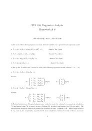
Example 1.1.1 (Wölfer’s sunspot numbers) In Figure 1.1, the number <strong>of</strong> sunspots<br />
(that is, dark spots observed on the surface <strong>of</strong> the sun) observed annually are plotted<br />
2
0 50 100 150<br />
•<br />
Number <strong>of</strong> Sun spots<br />
• •••<br />
•<br />
•<br />
•<br />
•<br />
•••• •<br />
•<br />
•<br />
• •<br />
• •<br />
• •<br />
•<br />
• • •<br />
• • •<br />
• •<br />
• ••• • •<br />
• •<br />
• • •<br />
• • •<br />
•<br />
•<br />
•<br />
•<br />
•<br />
• •<br />
• •<br />
•• •<br />
••<br />
•<br />
•<br />
•<br />
•<br />
• •<br />
•<br />
•<br />
• •<br />
•<br />
•<br />
• • •<br />
• •<br />
• •<br />
••<br />
•<br />
• •<br />
•<br />
• •<br />
••<br />
• •<br />
•<br />
•<br />
• •<br />
••<br />
•<br />
• •<br />
•<br />
••••• •••<br />
•<br />
•<br />
• • •<br />
•<br />
•<br />
• •<br />
•• •• ••<br />
•<br />
•<br />
• •<br />
•<br />
•<br />
•<br />
•<br />
•<br />
•<br />
•<br />
• •<br />
••<br />
•<br />
•<br />
• •<br />
• •<br />
• •<br />
••<br />
• •<br />
•<br />
•<br />
• •<br />
•<br />
•<br />
•<br />
•<br />
•<br />
•<br />
•<br />
•<br />
•<br />
•<br />
•<br />
•••<br />
•<br />
•<br />
• •<br />
•<br />
• ••<br />
• •<br />
• •<br />
•<br />
•<br />
• • •<br />
•<br />
•<br />
• •<br />
• • • •<br />
•<br />
• • ••<br />
•• •• •<br />
• ••• •<br />
•<br />
• •<br />
•<br />
•<br />
•<br />
• •<br />
• • •<br />
•<br />
•<br />
• • • •<br />
••<br />
•<br />
•<br />
•<br />
•<br />
• •<br />
• • •<br />
•<br />
•<br />
••<br />
•<br />
•<br />
•<br />
•<br />
•<br />
•<br />
• •<br />
•<br />
•<br />
•<br />
• • • •<br />
• •<br />
• •<br />
• ••<br />
• •<br />
• •<br />
•<br />
•<br />
•<br />
••<br />
1700 1750 1800 1850<br />
time<br />
1900 1950 2000<br />
Figure 1.1: Wölfer’s sunspot numbers from 1700 to 1994.<br />
against time. The horizontal axis labels time in years, while the vertical axis represents<br />
the observed values xt <strong>of</strong> the random variable<br />
Xt = # <strong>of</strong> sunspots at time t, t = 1700, . . . , 1994.<br />
The figure is called a time series plot. It is a useful device for a preliminary analysis.<br />
Sunspot numbers are used to explain magnetic oscillations on the sun surface.<br />
To reproduce a version <strong>of</strong> the time series plot in Figure 1.1 using the free s<strong>of</strong>tware package<br />
R 1 , download the file sunspots.dat from the course webpage and type the following<br />
commands:<br />
> spots = read.table("sunspots.dat")<br />
> spots = ts(spots, start=1700, frequency=1)<br />
> plot(spots, xlab="time", ylab="", main="Number <strong>of</strong> Sun spots")<br />
In the first line, the file sunspots.dat is read into the object spots, which is then in the<br />
second line transformed into a time series object using the function ts(). Using start<br />
sets the starting value for the x-axis to a prespecified number, while frequency presets<br />
the number <strong>of</strong> observations for one unit <strong>of</strong> time. (Here: one annual observation.) Finally,<br />
plot is the standard plotting command in R, where xlab and ylab determine the labels<br />
for the x-axis and y-axis, respectively, and main gives the headline.<br />
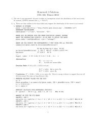
Example 1.1.2 (Canadian lynx data) The time series plot in Figure 1.2 comes from<br />
a biological data set. It contains the annual returns <strong>of</strong> lynx at auction in London by the<br />
Hudson Bay Company from 1821–1934 (on a log 10 scale). Here, we have observations <strong>of</strong><br />
the stochastic process<br />
Xt = log 10(number <strong>of</strong> lynx trapped at time 1820 + t), t = 1, . . . , 114.<br />
1 Downloads are available at http://cran.r-project.org.<br />
3<br />
•<br />
•<br />
•<br />
• •
2.0 2.5 3.0 3.5<br />
•<br />
• •<br />
•<br />
•<br />
•<br />
•<br />
• •<br />
•<br />
•<br />
•<br />
•<br />
•<br />
•<br />
• •<br />
•<br />
•<br />
•<br />
•<br />
•<br />
•<br />
•<br />
•<br />
•<br />
• •<br />
•<br />
•• •<br />
•<br />
•<br />
•<br />
•<br />
•<br />
•<br />
Number <strong>of</strong> trapped lynx<br />
•<br />
•<br />
•<br />
••<br />
•<br />
•<br />
•<br />
•<br />
•<br />
•<br />
•<br />
•<br />
•<br />
•<br />
••<br />
•<br />
•<br />
•<br />
• •<br />
•<br />
•<br />
•<br />
•<br />
•<br />
•<br />
•<br />
•<br />
•<br />
•<br />
•<br />
•<br />
•<br />
•<br />
• •<br />
•<br />
•<br />
•<br />
•<br />
•<br />
•<br />
•<br />
• •<br />
•<br />
•<br />
• •<br />
•<br />
•<br />
• •<br />
••<br />
•<br />
0 20 40 60 80 100<br />
Figure 1.2: Number <strong>of</strong> lynx trapped in the MacKenzie River district between 1821 and<br />
1934.<br />
The data is used as an estimate for the number <strong>of</strong> lynx trapped along the MacKenzie River<br />
in Canada. This estimate is <strong>of</strong>ten used as a proxy for the true population size <strong>of</strong> the lynx.<br />
A similar time series plot could be obtained for the snowshoe rabbit, the primary food<br />
source <strong>of</strong> the Canadian lynx, hinting at an intricate predator-prey relationship.<br />
Assuming that the data is stored in the file lynx.dat, the corresponding R commands<br />
leading to the time series plot in Figure 1.2 are<br />
> lynx = read.table("lynx.dat")<br />
> lynx = ts(log10(lynx), start=1821, frequency=1)<br />
> plot(lynx, xlab="", ylab="", main="Number <strong>of</strong> trapped lynx")<br />
Example 1.1.3 (Treasury bills) Another important field <strong>of</strong> application for time series<br />
analysis lies in the area <strong>of</strong> finance. To hedge the risks <strong>of</strong> portfolios, investors commonly<br />
use short-term risk-free interest rates such as the yields <strong>of</strong> three-month, six-month, and<br />
twelve-month Treasury bills plotted in Figure 1.3. The (multivariate) data displayed<br />
consists <strong>of</strong> 2,386 weekly observations from July 17, 1959, to December 31, 1999. Here,<br />
Xt = (Xt,1, Xt,2, Xt,3), t = 1, . . . , 2386,<br />
where Xt,1, Xt,2 and Xt,3 denote the three-month, six-month, and twelve-month yields at<br />
time t, respectively. It can be seen from the graph that all three Treasury bills are moving<br />
very similarly over time, implying a high correlation between the components <strong>of</strong> Xt.<br />
To produce the three-variate time series plot in Figure 1.3, you can use the R code<br />
> bills03 = read.table("bills03.dat");<br />
> bills06 = read.table("bills06.dat");<br />
> bills12 = read.table("bills12.dat");<br />
4<br />
•<br />
•<br />
•<br />
••<br />
•<br />
•<br />
•<br />
•<br />
•<br />
•<br />
•<br />
•<br />
•<br />
•<br />
•<br />
•<br />
•
5 10 15<br />
2 4 6 8 10 12 14 16<br />
4 6 8 10 12 14<br />
Yields <strong>of</strong> 3-month Treasury Bills<br />
0 500 1000<br />
(a)<br />
1500 2000<br />
Yields <strong>of</strong> 6-month Treasury Bills<br />
0 500 1000<br />
(b)<br />
1500 2000<br />
Yields <strong>of</strong> 12-month Treasury Bills<br />
0 500 1000 1500 2000<br />
(c)<br />
Figure 1.3: Yields <strong>of</strong> Treasury bills from July 17, 1959, to December 31, 1999.<br />
5
4.5 5.0 5.5 6.0 6.5 7.0<br />
The Standard and Poor’s 500 Index<br />
0 2000 4000 6000<br />
Figure 1.4: S&P 500 from January 3, 1972, to December 31, 1999.<br />
> par(mfrow=c(3,1))<br />
> plot.ts(bills03, xlab="(a)", ylab="",<br />
main="Yields <strong>of</strong> 3-month Treasury Bills")<br />
> plot.ts(bills06, xlab="(b)", ylab="",<br />
main="Yields <strong>of</strong> 6-month Treasury Bills")<br />
> plot.ts(bills12, xlab="(c)", ylab="",<br />
main="Yields <strong>of</strong> 12-month Treasury Bills")<br />
It is again assumed that the data can be found in the corresponding files bills03.dat,<br />
bills06.dat and bills12.dat. The command line par(mfrow=c(3,1)) is used to set<br />
up the graphics. It enables you to save three different plots in the same file.<br />
Example 1.1.4 (S&P 500) The Standard and Poor’s 500 index (S&P 500) is a valueweighted<br />
index based on the prices <strong>of</strong> 500 stocks that account for approximately 70%<br />
<strong>of</strong> the U.S. equity market capitalization. It is a leading economic indicator and is also<br />
used to hedge market portfolios. Figure 1.4 contains the 7,076 daily S&P 500 closing<br />
prices from January 3, 1972, to December 31, 1999, on a natural logarithm scale. We are<br />
consequently looking at the time series plot <strong>of</strong> the process<br />
Xt = ln(closing price <strong>of</strong> S&P 500 at time t), t = 1, . . . , 7076.<br />
Note that the logarithm transform has been applied to make the returns directly comparable<br />
to the percentage <strong>of</strong> investment return. The time series plot can be reproduced in<br />
R using the file sp500.dat.<br />
There are countless other examples from all areas <strong>of</strong> science. To develop a theory<br />
capable <strong>of</strong> handling broad applications, the statistician needs to rely on a mathematical<br />
framework that can explain phenomena such as<br />
• trends (apparent in Example 1.1.4);<br />
6
• seasonal or cyclical effects (apparent in Examples 1.1.1 and 1.1.2);<br />
• random fluctuations (all Examples);<br />
• dependence (all Examples?).<br />
The classical approach taken in time series analysis is to postulate that the stochastic<br />
process (Xt)t∈T under investigation can be divided into deterministic trend and seasonal<br />
components plus a centered random component, giving rise to the model<br />
Xt = mt + st + Yt, t ∈ T, (1.1.1)<br />
where (mt)t∈T denotes the trend function (“mean component”), (st)t∈T the seasonal effects<br />
and (Yt)t∈T a (zero mean) stochastic process. After an appropriate model has been chosen,<br />
the statistician may aim at<br />
• estimating the model parameters for a better understanding <strong>of</strong> the time series;<br />
• forecasting future values, for example, to develop investing strategies;<br />
• checking the goodness <strong>of</strong> fit to the data to confirm that the chosen model is indeed<br />
appropriate.<br />
We shall deal in detail with estimation procedures and forecasting techniques in later<br />
chapters <strong>of</strong> these notes. The rest <strong>of</strong> this chapter will be devoted to introducing the classes<br />
<strong>of</strong> strictly and weakly stationary stochastic processes (in Section 1.2) and to providing<br />
tools to eliminate trends and seasonal components from a given time series (in Sections<br />
1.3 and 1.4), while some goodness <strong>of</strong> fit tests will be presented in Section 1.5.<br />
1.2 Stationary <strong>Time</strong> <strong>Series</strong><br />
Fitting solely independent and identically distributed random variables to data is too<br />
narrow a concept. While, on one hand, they allow for a somewhat nice and easy mathematical<br />
treatment, their use is, on the other hand, <strong>of</strong>ten hard to justify in applications.<br />
Our goal is therefore to introduce a concept that keeps some <strong>of</strong> the desirable properties<br />
<strong>of</strong> independent and identically distributed random variables (“regularity”), but that also<br />
considerably enlarges the class <strong>of</strong> stochastic processes to choose from by allowing dependence<br />
as well as varying distributions. Dependence between two random variables X and<br />
Y is usually measured in terms <strong>of</strong> the covariance function<br />
Cov(X, Y ) = E (X − E[X])(Y − E[Y ]) <br />
and the correlation function<br />
Corr(X, Y ) =<br />
Cov(X, Y )<br />
Var(X)Var(Y ) .<br />
With these notations, we can now introduce the classes <strong>of</strong> strictly and weakly dependent<br />
stochastic processes.<br />
7
Definition 1.2.1 (Strict Stationarity) A stochastic process (Xt)t∈T is called strictly<br />
stationary if, for all t1, . . . , tn ∈ T and h such that t1 + h, . . . , tn + h ∈ T , it holds that<br />
(Xt1, . . . , Xtn) D = (Xt1+h, . . . , Xtn+h).<br />
That is, the so-called finite-dimensional distributions <strong>of</strong> the process are invariant under<br />
time shifts. Here = D indicates equality in distribution.<br />
The definition in terms <strong>of</strong> the finite-dimensional distribution can be reformulated equivalently<br />
in terms <strong>of</strong> the cumulative joint distribution function equalities<br />
P (Xt1 ≤ x1, . . . , Xtn ≤ xn) = P (Xt1+h ≤ x1, . . . , Xtn+h ≤ xn)<br />
holding true for all x1, . . . , xn ∈ R, t1, . . . , tn ∈ T and h such that t1 + h, . . . , tn + h ∈ T .<br />
This can be quite difficult to check for a given time series, especially if the generating<br />
mechanism <strong>of</strong> a time series is far from simple, since too many model parameters have to<br />
be estimated from the available data rendering concise statistical statements impossible.<br />
A possible exception is provided by the case <strong>of</strong> independent and identically distributed<br />
random variables.<br />
To get around these difficulties, a time series analyst will commonly only specify the<br />
first- and second-order moments <strong>of</strong> the joint distributions. Doing so then leads to the<br />
notion <strong>of</strong> weak stationarity.<br />
Definition 1.2.2 (Weak Stationarity) A stochastic process (Xt)t∈T is called weakly<br />
stationary if<br />
• the second moments are finite: E[X 2 t ] < ∞ for all t ∈ T ;<br />
• the means are constant: E[Xt] = m for all t ∈ T ;<br />
• the covariance <strong>of</strong> Xt and Xt+h depends on h only:<br />
γ(h) = γX(h) = Cov(Xt, Xt+h), h ∈ T such that t + h ∈ T,<br />
is independent <strong>of</strong> t ∈ T and is called the autocovariance function (ACVF). Moreover,<br />
ρ(h) = ρX(h) = γ(h)<br />
, h ∈ T,<br />
γ(0)<br />
is called the autocorrelation function (ACF).<br />
Remark 1.2.1 If (Xt)t∈T is a strictly stationary stochastic process with finite second<br />
moments, then it is also weakly stationary. The converse is not necessarily true. If<br />
(Xt)t∈T , however, is weakly stationary and Gaussian, then it is also strictly stationary.<br />
Recall that a stochastic process is called Gaussian if, for any t1, . . . , tn ∈ T , the random<br />
vector (Xt1, . . . , Xtn) is multivariate normally distributed.<br />
This section is concluded with examples <strong>of</strong> stationary and nonstationary stochastic<br />
processes.<br />
8
−0.5 0.0 0.5<br />
0 20 40 60 80 100<br />
−0.5 0.0 0.5 1.0<br />
0 20 40 60 80 100<br />
−1.0 −0.5 0.0 0.5 1.0<br />
0 20 40 60 80 100<br />
Figure 1.5: 100 simulated values <strong>of</strong> the cyclical time series (left panel), the stochastic<br />
amplitude (middle panel), and the sine part (right panel).<br />
Example 1.2.1 (White Noise) Let (Zt)t∈Z be a sequence <strong>of</strong> real-valued, pairwise uncorrelated<br />
random variables with E[Zt] = 0 and 0 < Var(Zt) = σ 2 < ∞ for all t ∈ Z.<br />
Then (Zt)t∈Z is called white noise, which shall be abbreviated by (Zt)t∈Z ∼ WN(0, σ 2 ). It<br />
defines a centered, weakly stationary process with ACVF and ACF given by<br />
γ(h) =<br />
σ 2 , h = 0,<br />
0, h = 0,<br />
and ρ(h) =<br />
1, h = 0,<br />
0, h = 0,<br />
respectively. If the (Zt)t∈Z are moreover independent and identically distributed, they are<br />
called iid noise, shortly (Zt)t∈Z ∼ IID(0, σ 2 ). The left panel <strong>of</strong> Figure 1.6 displays 1000<br />
observations <strong>of</strong> an iid noise sequence (Zt)t∈Z based on standard normal random variables.<br />
The corresponding R commands to produce the plot are<br />
> z = rnorm(1000, 0, 1)<br />
> plot.ts(z, xlab="", ylab="", main="")<br />
The command rnorm simulates here 1000 normal random variables with mean 0 and variance<br />
1. There are various built-in random variable generators in R such as the functions<br />
runif(n,a,b) and rbinom(n,m,p) which simulate the n values <strong>of</strong> a uniform distribution<br />
on the interval (a, b) and a binomial distribution with repetition parameter m and success<br />
probability p, respectively.<br />
Example 1.2.2 (Cyclical <strong>Time</strong> <strong>Series</strong>) Let A and B be uncorrelated random variables<br />
with zero mean and variances Var(A) = Var(B) = σ 2 , and let λ ∈ R be a frequency<br />
parameter. Define<br />
Xt = A cos(λt) + B sin(λt), t ∈ R.<br />
The resulting stochastic process (Xt)t∈R is then weakly stationary. Since sin(λt + ϕ) =<br />
sin(ϕ) cos(λt) + cos(ϕ) sin(λt), the process can be represented as<br />
Xt = R sin(λt + ϕ), t ∈ R,<br />
so that R is the stochastic amplitude and ϕ ∈ [−π, π] the stochastic phase <strong>of</strong> a sinusoid.<br />
Easy computations show that we must have A = R sin(ϕ) and B = R cos(ϕ). In the left<br />
panel <strong>of</strong> Figure 1.5, 100 observed values <strong>of</strong> a series (Xt)t∈Z have been displayed. Therein,<br />
9
−3 −2 −1 0 1 2 3<br />
0 200 400 600 800 1000<br />
0 10 20 30<br />
0 200 400 600 800 1000<br />
Figure 1.6: 1000 simulated values <strong>of</strong> iid N (0, 1) noise (left panel) and a random walk<br />
with iid N (0, 1) innovations (right panel).<br />
we have used λ = π/25, while R and ϕ are random variables uniformly distributed on the<br />
interval (−.5, 1) and (0, 1), respectively. The middle panel shows the realization <strong>of</strong> R, the<br />
right panel the realization <strong>of</strong> sin(λt+ϕ). Using cyclical time series bears great advantages<br />
when seasonal effects, such as annually recurrent phenomena, have to be modeled. You<br />
can apply the following R commands:<br />
> t = 1:100; R = runif(100,-.5,1); phi = runif(100,0,1); lambda = pi/25<br />
> cyc = R*sin(lambda*t+phi)<br />
> plot.ts(cyc, xlab="", ylab="")<br />
This produces the left panel <strong>of</strong> Figure 1.5. The middle and right panels follow in a similar<br />
fashion.<br />
Example 1.2.3 (Random Walk) Let (Zt)t∈N ∼ WN(0, σ 2 ). Let S0 = 0 and<br />
St = Z1 + . . . + Zt, t ∈ N.<br />
The resulting stochastic process (St)t∈N0 is called a random walk and is the most important<br />
nonstationary time series. Indeed, it holds here that, for h > 0,<br />
Cov(St, St+h) = Cov(St, St + Rt,h) = tσ 2 ,<br />
where Rt,h = Zt+1 + . . . + Zt+h, and the ACVF obviously depends on t. In R, you may<br />
construct a random walk, for example, with the following simple command that utilizes<br />
the 1000 normal observations stored in the array z <strong>of</strong> Example 1.2.1.<br />
> rw = cumsum(z)<br />
The function cumsum takes as input an array and returns as output an array <strong>of</strong> the same<br />
length that contains as its jth entry the sum <strong>of</strong> the first j input entries. The resulting<br />
time series plot is shown in the right panel <strong>of</strong> Figure 1.6.<br />
10
In Chapter 3 below, we shall discuss in detail so-called autoregressive moving average<br />
processes which have become a central building block in time series analysis. They are<br />
constructed from white noise sequences by an application <strong>of</strong> a set <strong>of</strong> stochastic difference<br />
equations similar to the ones defining the random walk (St)t∈N0 <strong>of</strong> Example 1.2.3.<br />
In general, however, the true parameters <strong>of</strong> a stationary stochastic process (Xt)t∈T are<br />
unknown to the statistician. Therefore, they have to be estimated from a realization<br />
x1, . . . , xn. We shall mainly work with the following set <strong>of</strong> estimators. The sample mean<br />
<strong>of</strong> x1, . . . , xn is defined as<br />
¯x = 1<br />
n<br />
n<br />
xt.<br />
The sample autocovariance function (sample ACVF) is given by<br />
t=1<br />
ˆγ(h) = 1 n−h<br />
(xt+h − ¯x)(xt − ¯x), h = 0, 1, . . . , n − 1. (1.2.1)<br />
n<br />
t=1<br />
Finally, the sample autocorrelation function (sample ACF) is<br />
ˆρ(h) = ˆγ(h)<br />
, h = 0, 1, . . . , n − 1.<br />
ˆγ(0)<br />
Example 1.2.4 Let (Zt)t∈Z be a sequence <strong>of</strong> independent standard normally distributed<br />
random variables (see the left panel <strong>of</strong> Figure 1.6 for a typical realization <strong>of</strong> size n = 1,000).<br />
Then, clearly, γ(0) = ρ(0) = 1 and γ(h) = ρ(h) = 0 whenever h = 0. Table 1.1 gives the<br />
corresponding estimated values ˆγ(h) and ˆρ(h) for h = 0, 1, . . . , 5. The estimated values<br />
h 0 1 2 3 4 5<br />
ˆγ(h) 1.069632 0.072996 −0.000046 −0.000119 0.024282 0.0013409<br />
ˆρ(h) 1.000000 0.068244 −0.000043 −0.000111 0.022700 0.0012529<br />
Table 1.1: Estimated ACVF and ACF for selected values <strong>of</strong> h.<br />
are all very close to the true ones, indicating that the estimators work reasonably well for<br />
n = 1,000. Indeed it can be shown that they are asymptotically unbiased and consistent.<br />
Moreover, the sample autocorrelations ˆρ(h) are approximately normal with zero mean<br />
and variance 1/1000. See also Theorem 1.2.1 below. In R, you may use the function acf<br />
to compute the sample ACF.<br />
Theorem 1.2.1 Let (Zt)t∈Z ∼ WN(0, σ 2 ) and let h = 0. Under a general set <strong>of</strong> conditions,<br />
it holds that the sample ACF at lag h, ˆρ(h), is for large n approximately normally<br />
distributed with zero mean and variance 1/n.<br />
Theorem 1.2.1 and Example 1.2.4 suggest a first method to assess whether or not a<br />
given data set can be modeled conveniently by a white noise sequence: for a white noise<br />
sequence, approximately 95% <strong>of</strong> the sample ACFs should be within the the confidence<br />
interval ±2/ √ n. Using the data files on the course webpage, you can compute with R<br />
the corresponding sample ACFs to check for whiteness <strong>of</strong> the underlying time series. We<br />
will come back to properties <strong>of</strong> the sample ACF in Chapter 2.<br />
11
6 7 8 9 10 11 12<br />
1880 1900 1920 1940 1960<br />
−2 −1 0 1 2<br />
1880 1900 1920 1940 1960<br />
Figure 1.7: Annual water levels <strong>of</strong> Lake Huron (left panel) and the residual plot obtained<br />
from fitting a linear trend to the data (right panel).<br />
1.3 Eliminating Trend Components<br />
In this section we develop three different methods to estimate the trend <strong>of</strong> a time series<br />
model. We assume that it makes sense to postulate the model (1.1.1) with st = 0 for all<br />
t ∈ T , that is,<br />
Xt = mt + Yt, t ∈ T, (1.3.1)<br />
where (without loss <strong>of</strong> generality) E[Yt] = 0. In particular, we will discuss three different<br />
methods, (1) the least squares estimation <strong>of</strong> mt, (2) smoothing by means <strong>of</strong> moving averages<br />
and (3) differencing.<br />
Method 1 (Least squares estimation) It is <strong>of</strong>ten useful to assume that a trend component<br />
can be modeled appropriately by a polynomial,<br />
mt = b0 + b1t + . . . + bpt p , p ∈ N0.<br />
In this case, the unknown parameters b0, . . . , bp can be estimated by the least squares<br />
method. Combined, they yield the estimated polynomial trend<br />
ˆmt = ˆ b0 + ˆ b1t + . . . + ˆ bpt p , t ∈ T,<br />
where ˆ b0, . . . , ˆ bp denote the corresponding least squares estimates. Note that we do not<br />
estimate the order p. It has to be selected by the statistician—for example, by inspecting<br />
the time series plot. The residuals ˆ Yt can be obtained as<br />
ˆYt = Xt − ˆmt = Xt − ˆ b0 − ˆ b1t − . . . − ˆ bpt p , t ∈ T.<br />
How to assess the goodness <strong>of</strong> fit <strong>of</strong> the fitted trend will be subject <strong>of</strong> Section 1.5 below.<br />
12
Example 1.3.1 (Level <strong>of</strong> Lake Huron) The left panel <strong>of</strong> Figure 1.7 contains the time<br />
series <strong>of</strong> the annual average water levels in feet (reduced by 570) <strong>of</strong> Lake Huron from 1875<br />
to 1972. We are dealing with a realization <strong>of</strong> the process<br />
Xt = (Average water level <strong>of</strong> Lake Huron in the year 1874 + t) − 570, t = 1, . . . , 98.<br />
There seems to be a linear decline in the water level and it is therefore reasonable to fit a<br />
polynomial <strong>of</strong> order one to the data. Evaluating the least squares estimators provides us<br />
with the values<br />
ˆ b0 = 10.202 and ˆ b1 = −0.0242<br />
for the intercept and the slope, respectively. The resulting observed residuals ˆyt = ˆ Yt(ω)<br />
are plotted against time in the right panel <strong>of</strong> Figure 1.7. There is no apparent trend left<br />
in the data. On the other hand, the plot does not strongly support the stationarity <strong>of</strong> the<br />
residuals. Additionally, there is evidence <strong>of</strong> dependence in the data.<br />
To reproduce the analysis in R, assume that the data is stored in the file lake.dat.<br />
Then use the following commands.<br />
> lake = read.table("lake.dat")<br />
> lake = ts(lake, start=1875)<br />
> t = 1:length(lake)<br />
> lsfit = lm(lake ∼ t)<br />
> plot(t, lake, xlab="", ylab="", main="")<br />
> lines(lsfit$fit)<br />
The function lm fits a linear model or regression line to the Lake Huron data. To plot both<br />
the original data set and the fitted regression line into the same graph, you can first plot<br />
the water levels and then use the lines function to superimpose the fit. The residuals<br />
corresponding to the linear model fit can be accessed with the command lsfit$resid.<br />
Method 2 (Smoothing with Moving Averages) Let (Xt)t∈Z be a stochastic process<br />
following model (1.3.1). Choose q ∈ N0 and define the two-sided moving average<br />
Wt = 1<br />
2q + 1<br />
q<br />
Xt+j, t ∈ Z. (1.3.2)<br />
j=−q<br />
The random variables Wt can be utilized to estimate the trend component mt in the<br />
following way. First note that<br />
Wt = 1<br />
2q + 1<br />
q<br />
j=−q<br />
mt+j + 1<br />
2q + 1<br />
q<br />
Yt+j ≈ mt,<br />
assuming that the trend is locally approximately linear and that the average <strong>of</strong> the Yt<br />
over the interval [t − q, t + q] is close to zero. Therefore, mt can be estimated by<br />
j=−q<br />
ˆmt = Wt, t = q + 1, . . . , n − q.<br />
13
7 8 9 10 11<br />
−1.0 −0.5 0.0 0.5 1.0<br />
1880 1900 1920 1940 1960<br />
1880 1900 1920 1940 1960<br />
7 8 9 10 11<br />
−2 −1 0 1 2 3<br />
1880 1900 1920 1940 1960<br />
1880 1900 1920 1940 1960<br />
8.5 9.0 9.5 10.0<br />
−2 −1 0 1 2<br />
1880 1900 1920 1940 1960<br />
1880 1900 1920 1940 1960<br />
Figure 1.8: The two-sided moving average filters Wt for the Lake Huron data (upper<br />
panel) and their residuals (lower panel) with bandwidth q = 2 (left), q = 10 (middle) and<br />
q = 35 (right).<br />
Notice that there is no possibility <strong>of</strong> estimating the first q and last n − q drift terms due<br />
to the two-sided nature <strong>of</strong> the moving averages. In contrast, one can also define one-sided<br />
moving averages by letting<br />
ˆm1 = X1, ˆmt = aXt + (1 − a) ˆmt−1, t = 2, . . . , n.<br />
Figure 1.8 contains estimators ˆmt based on the two-sided moving averages for the Lake<br />
Huron data <strong>of</strong> Example 1.3.1 for selected choices <strong>of</strong> q (upper panel) and the corresponding<br />
estimated residuals (lower panel).<br />
The moving average filters for this example can be produced in R in the following way:<br />
> t = 1:length(lake)<br />
> ma2 = filter(lake, sides=2, rep(1,5)/5)<br />
> ma10 = filter(lake, sides=2, rep(1,21)/21)<br />
> ma35 = filter(lake, sides=2, rep(1,71)/71)<br />
> plot(t, ma2, xlab="", ylab="")<br />
> lines(ma10); lines(ma35)<br />
Therein, sides determines if a one- or two-sided filter is going to be used. The phrase<br />
rep(1,5) creates a vector <strong>of</strong> length 5 with each entry being equal to 1.<br />
More general versions <strong>of</strong> the moving average smoothers can be obtained in the following<br />
way. Observe that in the case <strong>of</strong> the two-sided version Wt each variable Xt−q, . . . , Xt+q<br />
obtains a “weight” aj = (2q + 1) −1 . The sum <strong>of</strong> all weights thus equals one. The same<br />
is true for the one-sided moving averages with weights a and 1 − a. Generally, one can<br />
14
hence define a smoother by letting<br />
ˆmt =<br />
q<br />
ajXt+j, t = q + 1, . . . , n − q, (1.3.3)<br />
j=−q<br />
where a−q + . . . + aq = 1. These general moving averages (two-sided and one-sided) are<br />
commonly referred to as linear filters. There are countless choices for the weights. The<br />
one here, aj = (2q + 1) −1 , has the advantage that linear trends pass undistorted. In the<br />
next example, we introduce a filter which passes cubic trends without distortion.<br />
Example 1.3.2 (Spencer’s 15-point moving average) Suppose that the filter in display<br />
(1.3.3) is defined by weights satisfying aj = 0 if |j| > 7, aj = a−j and<br />
(a0, a1, . . . , a7) = 1<br />
(74, 67, 46, 21, 3, −5, −6, −3).<br />
320<br />
Then, the corresponding filters passes cubic trends mt = b0 + b1t + b2t 2 + b3t 3 undistorted.<br />
To see this, observe that<br />
7<br />
aj = 1 and<br />
j=−7<br />
7<br />
j r aj = 0, r = 1, 2, 3.<br />
j=−7<br />
Now apply Proposition 1.3.1 below to arrive at the conclusion. Assuming that the observations<br />
are in data, you may use the R commands<br />
> a =c(-3, -6, -5, 3, 21, 46, 67, 74, 67, 46, 21, 3, -5, -6, -3)/320<br />
> s15 = filter(data, sides=2, a)<br />
to apply Spencer’s 15-point moving average filter. This example also explains how to<br />
specify a general tailor-made filter for a given data set.<br />
Proposition 1.3.1 A linear filter (1.3.3) passes a polynomial <strong>of</strong> degree p if and only if<br />
<br />
aj = 1 and <br />
j r aj = 0, r = 1, . . . , p.<br />
j<br />
j<br />
Pro<strong>of</strong>. It suffices to show that <br />
j aj(t + j) r = t r for r = 0, . . . , p. Using the binomial<br />
theorem, we can write<br />
<br />
aj(t + j) r = <br />
j<br />
=<br />
= t r<br />
j<br />
r<br />
k=0<br />
aj<br />
r<br />
k=0<br />
<br />
r<br />
t<br />
k<br />
k<br />
<br />
r<br />
t<br />
k<br />
k j r−k<br />
<br />
<br />
ajj r−k<br />
<br />
for any r = 0, . . . , p if and only if the above conditions hold. This completes the pro<strong>of</strong>.✷<br />
15<br />
j
−2 −1 0 1 2<br />
1880 1900 1920 1940 1960<br />
−3 −2 −1 0 1 2<br />
1880 1900 1920 1940 1960<br />
Figure 1.9: <strong>Time</strong> series plots <strong>of</strong> the observed sequences (∇xt) in the left panel and (∇ 2 xt)<br />
in the right panel <strong>of</strong> the differenced Lake Huron data described in Example 1.3.1.<br />
Method 3 (Differencing) A third possibility to remove drift terms from a given time<br />
series is differencing. To this end, we introduce the difference operator ∇ as<br />
∇Xt = Xt − Xt−1 = (1 − B)Xt, t ∈ T,<br />
where B denotes the backshift operator BXt = Xt−1. Repeated application <strong>of</strong> ∇ is defined<br />
in the intuitive way:<br />
∇ 2 Xt = ∇(∇Xt) = ∇(Xt − Xt−1) = Xt − 2Xt−1 + Xt−2<br />
and, recursively, the representations follow also for higher powers <strong>of</strong> ∇. Suppose that you<br />
are applying the difference operator to a linear trend mt = b0 + b1t, then you obtain<br />
∇mt = mt − mt−1 = b0 + b1t − b0 − b1(t − 1) = b1<br />
which is a constant. Inductively, this leads to the conclusion that for a polynomial drift <strong>of</strong><br />
degree p, namely mt = p j=0 bjtj , we have that ∇pmt = p!bp and thus constant. Applying<br />
this technique to a stochastic process <strong>of</strong> the form (1.3.1) with a polynomial drift mt, yields<br />
then<br />
∇ p Xt = p!bp + ∇ p Yt, t ∈ T.<br />
This is a stationary process with mean p!bp. The plots in Figure 1.9 contain the first<br />
and second differences for the Lake Huron data. In R, they may be obtained from the<br />
commands<br />
> d1 = diff(lake)<br />
> d2 = diff(d1)<br />
> par(mfrow=c(1,2))<br />
> plot.ts(d1, xlab="", ylab="")<br />
> plot.ts(d2, xlab="", ylab="")<br />
The next example shows that the difference operator can also be applied to a random<br />
walk to create stationary data.<br />
16
Example 1.3.3 Let (St)t∈N0 be the random walk <strong>of</strong> Example 1.2.3. If we apply the difference<br />
operator ∇ to this stochastic process, we obtain<br />
∇St = St − St−1 = Zt, t ∈ N.<br />
In other words, ∇ does nothing else but recover the original white noise sequence that was<br />
used to build the random walk.<br />
1.4 Eliminating Trend and Seasonal Components<br />
Let us go back to the classical decomposition (1.1.1),<br />
Xt = mt + st + Yt, t ∈ T,<br />
with E[Yt] = 0. In this section, we shall discuss three methods that aim at estimating both<br />
the trend and seasonal components in the data. As additional requirement on (st)t∈T , we<br />
assume that<br />
d<br />
st+d = st, sj = 0,<br />
where d denotes the period <strong>of</strong> the seasonal component. (If we are dealing with yearly data<br />
sampled monthly, then obviously d = 12.) It is convenient to relabel the observations<br />
x1, . . . , xn in terms <strong>of</strong> the seasonal period d as<br />
j=1<br />
xj,k = xk+d(j−1).<br />
In the case <strong>of</strong> yearly data, observation xj,k thus represents the data point observed for<br />
the kth month <strong>of</strong> the jth year. For convenience we shall always refer to the data in this<br />
fashion even if the actual period is something other than 12.<br />
Method 1 (Small trend method) If the changes in the drift term appear to be small,<br />
then it is reasonable to assume that the drift in year j, say, mj is constant. As a natural<br />
estimator we can therefore apply<br />
ˆmj = 1<br />
d<br />
To estimate the seasonality in the data, one can in a second step utilize the quantities<br />
ˆsk = 1<br />
N<br />
d<br />
k=1<br />
xj,k.<br />
N<br />
(xj,k − ˆmj),<br />
j=1<br />
where N is determined by the equation n = Nd, provided that data has been collected<br />
over N full cycles. Direct calculations show that these estimators possess the property<br />
ˆs1 + . . . + ˆsd = 0 (as in the case <strong>of</strong> the true seasonal components st). To further assess<br />
the quality <strong>of</strong> the fit, one needs to analyze the observed residuals<br />
ˆyj,k = xj,k − ˆmj − ˆsk.<br />
17
500 1000 1500 2000 2500 3000<br />
1980 1982 1984 1986 1988 1990 1992<br />
6.5 7.0 7.5 8.0<br />
1980 1982 1984 1986 1988 1990 1992<br />
Figure 1.10: <strong>Time</strong> series plots <strong>of</strong> the red wine sales in Australia from January 1980 to<br />
October 1991 (left) and its log transformation with yearly mean estimates (right).<br />
Note that due to the relabeling <strong>of</strong> the observations and the assumption <strong>of</strong> a slowly changing<br />
trend, the drift component is solely described by the “annual” subscript j, while the<br />
seasonal component only contains the “monthly” subscript k.<br />
Example 1.4.1 (Australian wine sales) The left panel <strong>of</strong> Figure 1.10 shows the monthly<br />
sales <strong>of</strong> red wine (in kiloliters) in Australia from January 1980 to October 1991. Since<br />
there is an apparent increase in the fluctuations over time, the right panel <strong>of</strong> the same<br />
figure shows the natural logarithm transform <strong>of</strong> the data. There is clear evidence <strong>of</strong> both<br />
trend and seasonality. In the following, we will continue to work with the log transformed<br />
data. Using the small trend method as described above, we first estimate the annual<br />
means, which are already incorporated in the right time series plot <strong>of</strong> Figure 1.10. Note<br />
that there are only ten months <strong>of</strong> data available for the year 1991, so that the estimation<br />
has to be adjusted accordingly. The detrended data is shown in the left panel <strong>of</strong> Figure<br />
1.11. The middle plot in the same figure shows the estimated seasonal component, while<br />
the right panel displays the residuals. Even though the assumption <strong>of</strong> small changes in<br />
the drift is somewhat questionable, the residuals appear to look quite nice. They indicate<br />
that there is dependence in the data (see Section 1.5 below for more on this subject).<br />
Method 2 (Moving average estimation) This method is to be preferred over the<br />
first one whenever the underlying trend component is not constant. Three steps are to<br />
be applied to the data.<br />
1st Step: Trend estimation. At first, we focus on the removal <strong>of</strong> the trend component<br />
with the linear filters discussed in the previous section. If the period d is odd, then we<br />
can directly use ˆmt = Wt as in (1.3.2) with q specified by the equation d = 2q + 1. If the<br />
period d = 2q is even, then we slightly modify Wt and use<br />
ˆmt = 1<br />
d (.5xt−q + xt−q+1 + . . . + xt+q−1 + .5xt+q), t = q + 1, . . . , n − q.<br />
18
−0.6 −0.2 0.0 0.2 0.4 0.6<br />
1980 1982 1984 1986 1988 1990 1992<br />
−1.0 −0.5 0.0 0.5<br />
1980 1982 1984 1986 1988 1990 1992<br />
−0.6 −0.2 0.0 0.2 0.4 0.6<br />
1980 1982 1984 1986 1988 1990 1992<br />
Figure 1.11: The detrended log series (left), the estimated seasonal component (center)<br />
and the corresponding residuals series (right) <strong>of</strong> the Australian red wine sales data.<br />
2nd Step: Seasonality estimation. To estimate the seasonal component, let<br />
Define now<br />
µk = 1<br />
N − 1<br />
N<br />
(xk+d(j−1) − ˆmk+d(j−1)), k = 1, . . . , q,<br />
j=2<br />
µk = 1<br />
N−1 <br />
(xk+d(j−1) − ˆmk+d(j−1)), k = q + 1, . . . , d.<br />
N − 1<br />
j=1<br />
ˆsk = µk − 1<br />
d<br />
d<br />
µℓ, k = 1, . . . , d,<br />
ℓ=1<br />
and set ˆsk = ˆsk−d whenever k > d. This will provide us with deseasonalized data which<br />
can be examined further. In the final step, any remaining trend can be removed from the<br />
data.<br />
3rd Step: Trend Reestimation. Apply any <strong>of</strong> the methods from Section 1.3.<br />
Method 3 (Differencing at lag d) Introducing the lag-d difference operator ∇d, defined<br />
by letting<br />
∇dXt = Xt − Xt−d = (1 − B d )Xt, t = d + 1, . . . , n,<br />
and assuming model (1.1.1), we arrive at the transformed random variables<br />
∇dXt = mt − mt−d + Yt − Yt−d, t = d + 1, . . . , n.<br />
Note that the seasonality is removed, since st = st−d. The remaining noise variables<br />
Yt − Yt−d are stationary and have zero mean. The new trend component mt − mt−d can<br />
be eliminated using any <strong>of</strong> the methods developed in Section 1.3.<br />
Example 1.4.2 (Australian wine sales) We revisit the Australian red wine sales data<br />
<strong>of</strong> Example 1.4.1 and apply the differencing techniques just established. The left plot <strong>of</strong><br />
Figure 1.12 shows the the data after an application <strong>of</strong> the operator ∇12. If we decide to<br />
estimate the remaining trend in the data with the differencing method from Section 1.3,<br />
we arrive at the residual plot given in the right panel <strong>of</strong> Figure 1.12. Note that the order <strong>of</strong><br />
application does not change the residuals, that is, ∇∇12xt = ∇12∇xt. The middle panel<br />
<strong>of</strong> Figure 1.12 displays the differenced data which still contains the seasonal component.<br />
19
−0.2 0.0 0.2 0.4<br />
0 20 40 60 80 100 120<br />
−0.8 −0.4 0.0 0.2 0.4<br />
0 20 40 60 80 100 120 140<br />
−0.4 −0.2 0.0 0.2 0.4<br />
0 20 40 60 80 100 120<br />
Figure 1.12: The differenced observed series ∇12xt (left), ∇xt (middle) and ∇∇12xt =<br />
∇12∇xt (right) for the Australian red wine sales data.<br />
1.5 Assessing the Residuals<br />
In this subsection, we introduce several goodness-<strong>of</strong>-fit tests to further analyze the residuals<br />
obtained after the elimination <strong>of</strong> trend and seasonal components. The main objective<br />
is to determine whether or not these residuals can be regarded as obtained from a sequence<br />
<strong>of</strong> independent, identically distributed random variables or if there is dependence<br />
in the data. Throughout we denote by Y1, . . . , Yn the residuals and by y1, . . . , yn a typical<br />
realization.<br />
Method 1 (The sample ACF) We have seen in Example 1.2.4 that, for j = 0, the<br />
estimators ˆρ(j) <strong>of</strong> the ACF ρ(j) are asymptotically independent and normally distributed<br />
with mean zero and variance n −1 , provided the underlying residuals are independent and<br />
identically distributed with a finite variance. Therefore, plotting the sample ACF for<br />
a certain number <strong>of</strong> lags, say h, we expect that approximately 95% <strong>of</strong> these values are<br />
within the bounds ±1.96/ √ n. The R function acf helps you to perform this analysis.<br />
(See Theorem 1.2.1.)<br />
Method 2 (The Portmanteau test) The Portmanteau test is based on the test statistic<br />
Q = n<br />
h<br />
ˆρ 2 (j).<br />
j=1<br />
Using the fact that the variables √ nˆρ(j) are asymptotically standard normal, it becomes<br />
apparent that Q itself can be approximated with a chi-squared distribution possessing<br />
h degrees <strong>of</strong> freedom. We now reject the hypothesis <strong>of</strong> independent and identically distributed<br />
residuals at the level α if Q > χ 2 1−α(h), where χ 2 1−α(h) is the 1 − α quantile <strong>of</strong><br />
the chi-squared distribution with h degrees <strong>of</strong> freedom. Several refinements <strong>of</strong> the original<br />
Portmanteau test have been established in the literature. We refer here only to the papers<br />
Ljung and Box (1978), and McLeod and Li (1983) for further information on this topic.<br />
Method 3 (The rank test) This test is very useful for finding linear trends. Denote by<br />
Π = #{(i, j) : Yi > Yj, i > j, i = 2, . . . , n}<br />
the random number <strong>of</strong> pairs (i, j) satisfying the conditions Yi > Yj and i > j. Clearly,<br />
there are n 1 = 2 2n(n − 1) pairs (i, j) such that i > j. If Y1, . . . , Yn are independent and<br />
20
identically distributed, then P (Yi > Yj) = 1/2 (assuming a continuous distribution). Now<br />
it follows that µΠ = E[Π] = 1<br />
4n(n − 1) and, similarly, σ2 1<br />
Π = Var(Π) = n(n − 1)(2n + 5).<br />
72<br />
Moreover, for large enough sample sizes n, Π has an approximate normal distribution with<br />
mean µΠ and variance σ2 Π . Consequently, one would reject the hypothesis <strong>of</strong> independent,<br />
identically distributed data at the level α if<br />
P =<br />
|Π − µΠ|<br />
σΠ<br />
> z1−α/2,<br />
where z1−α/2 denotes the 1 − α/2 quantile <strong>of</strong> the standard normal distribution.<br />
Method 4 (Tests for normality) If there is evidence that the data are generated by<br />
Gaussian random variables, one can create the qq plot to check for normality. It is based<br />
on a visual inspection <strong>of</strong> the data. To this end, denote by Y(1) < . . . < Y(n) the order<br />
statistics <strong>of</strong> the residuals Y1, . . . , Yn which are normally distributed with expected value<br />
µ and variance σ 2 . It holds that<br />
E[Y(j)] = µ + σE[X(j)], (1.5.1)<br />
where X(1) < . . . < X(n) are the order statistics <strong>of</strong> a standard normal distribution. The<br />
qq plot is defined as the graph <strong>of</strong> the pairs (E[X(1)], Y(1)), . . . , (E[X(n)], Y(n)). According<br />
to display (1.5.1), the resulting graph will be approximately linear with the squared<br />
correlation R 2 <strong>of</strong> the points being close to 1. The assumption <strong>of</strong> normality will thus be<br />
rejected if R 2 is “too” small. It is common to approximate E[X(j)] ≈ Φj = Φ −1 ((j −.5)/n)<br />
(Φ being the distribution function <strong>of</strong> the standard normal distribution) and the previous<br />
statement is made precise by letting<br />
R 2 =<br />
n<br />
j=1 (Y(j) − ¯ Y )Φj<br />
2<br />
n<br />
j=1 (Y(j) − ¯ Y ) 2 n<br />
j=1 Φ2 j<br />
where ¯ Y = 1<br />
n (Y1 + . . . + Yn). The critical values for R 2 are tabulated and can be found,<br />
for example in Shapiro and Francia (1972). The corresponding R function is qqnorm.<br />
1.6 Summary<br />
In this chapter, we have introduced the classical decomposition (1.1.1) <strong>of</strong> a time series<br />
into a drift component, a seasonal component and a sequence <strong>of</strong> residuals. We have<br />
provided methods to estimate the drift and the seasonality. Moreover, we have identified<br />
the class <strong>of</strong> stationary processes as a reasonably broad class <strong>of</strong> random variables. We have<br />
introduced several ways to check whether or not the resulting residuals can be considered<br />
to be independent, identically distributed. In Chapter 3, we will discuss in depth the<br />
class <strong>of</strong> autoregressive moving average (ARMA) processes, a parametric class <strong>of</strong> random<br />
variables that are at the center <strong>of</strong> linear time series analysis because they are able to<br />
capture a wide range <strong>of</strong> dependence structures and allow for a thorough mathematical<br />
treatment. Before, we are dealing with the properties <strong>of</strong> the sample mean, sample ACVF<br />
and ACF in the next chapter.<br />
21<br />
,
Chapter 2<br />
The Estimation <strong>of</strong> Mean and<br />
Covariances<br />
In this brief second chapter, we will collect some results concerning asymptotic properties<br />
<strong>of</strong> the sample mean and the sample ACVF. Throughout, we denote by (Xt)t∈Z a weakly<br />
stationary stochastic process with mean µ and ACVF γ. In Section 1.2 we have seen that<br />
such a process is completely characterized by these two quantities. We have estimated<br />
µ by computing the sample mean ¯x, and γ by ˆγ defined in (1.2.1). In the following, we<br />
shall discuss the properties <strong>of</strong> these estimators in more detail.<br />
2.1 Estimation <strong>of</strong> the Mean<br />
Assume that we have to find an appropriate guess for the unknown mean µ <strong>of</strong> some<br />
weakly stationary stochastic process (Xt)t∈Z. The sample mean ¯x, easily computed as<br />
the average <strong>of</strong> n observations x1, . . . , xn <strong>of</strong> the process, has been identified as suitable<br />
in Section 1.2. To investigate its theoretical properties, we need to analyze the random<br />
variable associated with it, that is,<br />
Two facts can be quickly established.<br />
¯Xn = 1<br />
n (X1 + . . . + Xn).<br />
• ¯ Xn is an unbiased estimator for µ, since<br />
E[ ¯ <br />
n<br />
<br />
1<br />
Xn] = E Xt =<br />
n<br />
1<br />
n<br />
t=1<br />
n<br />
t=1<br />
E[Xt] = 1<br />
nµ = µ.<br />
n<br />
This means that “on average”, we estimate the true but unknown µ. Notice that<br />
there is no difference in the computations between the standard case <strong>of</strong> independent<br />
and identically distributed random variables and the more general weakly stationary<br />
process considered here.<br />
22
• If γ(n) → 0 as n → ∞, then ¯ Xn is a consistent estimator for µ, since<br />
Var( ¯ <br />
n 1<br />
Xn) = Cov Xi,<br />
n<br />
1<br />
n<br />
<br />
Xj =<br />
n<br />
1<br />
n2 n n<br />
Cov(Xi, Xj)<br />
= 1<br />
n 2<br />
n<br />
i−j=−n<br />
i=1<br />
j=1<br />
(n − |i − j|)γ(i − j) = 1<br />
n<br />
i=1<br />
j=1<br />
n<br />
h=−n<br />
<br />
1 − |h|<br />
<br />
γ(h).<br />
n<br />
Now, the quantity on the right-hand side converges to zero as n → ∞ because<br />
γ(n) → 0 as n → ∞ by assumption. The first equality sign in the latter equation<br />
array follows from the fact that Var(X) = Cov(X, X) for any random variable X, the<br />
second equality sign uses that the covariance function is linear in both arguments.<br />
For the third equality, you can use that Cov(Xi, Xj) = γ(i−j) and that each γ(i−j)<br />
appears exactly n − |i − j| times in the double summation. Finally, the right-hand<br />
side is obtained by replacing i − j with h and pulling one n −1 inside the summation.<br />
In the standard case <strong>of</strong> independent and identically distributed random variables<br />
Var( ¯ X) = σ 2 . The condition γ(n) → 0 is automatically satisfied. However, in the<br />
general case <strong>of</strong> weakly stationary processes, it cannot be omitted.<br />
More can be proved using an appropriate set <strong>of</strong> assumptions. We only collect the results<br />
as a theorem without giving the pro<strong>of</strong>s.<br />
Theorem 2.1.1 Let (Xt)t∈Z be a weakly stationary stochastic process with mean µ and<br />
ACVF γ. Then, the following statements hold true as n → ∞.<br />
(a) If ∞ h=−∞ |γ(h)| < ∞, then<br />
nVar( ¯ Xn) →<br />
∞<br />
h=−∞<br />
(b) If the process is “close to Gaussianity”, then<br />
√ n( ¯ Xn − µ) ∼ AN(0, τ 2 n), τ 2 n =<br />
γ(h) = τ 2 ;<br />
n<br />
h=−n<br />
<br />
1 − |h|<br />
<br />
γ(h).<br />
n<br />
Here, ∼ AN(0, τ 2 n) stands for approximately normally distributed with mean zero and<br />
variance τ 2 n.<br />
Theorem 2.1.1 can be utilized to construct confidence intervals for the unknown mean<br />
parameter µ. To do so, we must, however, estimate the unknown variance parameter<br />
τn. For a large class <strong>of</strong> stochastic processes, it holds that τ 2 n converges to τ 2 as n → ∞.<br />
Therefore, we can use τ 2 as an approximation for τ 2 n. Moreover, τ 2 can be estimated by<br />
ˆτ 2 n =<br />
√ n<br />
<br />
h=− √ n<br />
<br />
1 − |h|<br />
<br />
ˆγ(h),<br />
n<br />
23
where ˆγ(h) denotes the ACVF estimator defined in (1.2.1). An approximate 95% confidence<br />
interval for µ can now be constructed as<br />
<br />
¯Xn − 1.96 ˆτn<br />
√n , ¯ Xn + 1.96 ˆτn<br />
<br />
√n .<br />
Example 2.1.1 (Autoregressive Processes) Let (Xt)t∈Z be given by the equations<br />
Xt − µ = φ(Xt−1 − µ) + Zt, t ∈ Z, (2.1.1)<br />
where (Zt)t∈Z ∼ WN(0, σ 2 ) and |φ| < 1. We will see in Chapter 3 that (Xt)t∈Z defines<br />
a weakly stationary process. Utilizing the stochastic difference equations (2.1.1), we can<br />
determine both mean and autocovariances. It holds that E[Xt] = φE[Xt−1] + µ(1 − φ).<br />
Since, by stationarity, E[Xt−1] can be substituted with E[Xt], we finally obtain that<br />
E[Xt] = µ, t ∈ Z.<br />
In the following we shall work with the process (Yt)t∈Z given by letting Yt = Xt − µ.<br />
Clearly, E[Yt] = 0. From the definition, it follows also that the covariances <strong>of</strong> (Xt)t∈Z and<br />
(Yt)t∈Z coincide. So let us first compute the second moment <strong>of</strong> Y 2<br />
t : We have<br />
E[Y 2<br />
t ] = E (φYt−1 + Zt) 2 = φ 2 E[Y 2<br />
t−1] + σ 2<br />
and consequently, since E[Y 2<br />
t−1] = E[Y 2<br />
t ] by weak stationarity <strong>of</strong> (Yt)t∈Z,<br />
E[Y 2<br />
t ] = σ2<br />
, t ∈ Z.<br />
1 − φ2 It becomes apparent from the latter equation, why the condition |φ| < 1 was needed in<br />
display (2.1.1). In the next step, we compute the autocovariance function. For h > 0, it<br />
holds that<br />
γ(h) = E[Yt+hYt] = E <br />
(φYt+h−1 + Zt+h)Yt = φE[Yt+h−1Yt] = φγ(h − 1) = φ h γ(0)<br />
after h iterations. But since γ(0) = E[Y 2<br />
t ], we obtain by symmetry <strong>of</strong> the ACVF that<br />
γ(h) = σ2φ |h|<br />
, h ∈ Z.<br />
1 − φ2 After these theoretical considerations, we can now construct a 95% confidence interval for<br />
the mean parameter µ. To check if Theorem 2.1.1 is applicable here, we need to check if<br />
the autocovariances are absolutely summable:<br />
τ 2 ∞<br />
= γ(h) = σ2<br />
1 − φ2 <br />
∞<br />
1 + 2 φ h<br />
<br />
h=−∞<br />
= σ2<br />
1 − φ 2<br />
1<br />
(1 + φ) =<br />
1 − φ<br />
h=1<br />
σ2 < ∞.<br />
(1 − φ) 2<br />
= σ2<br />
1 − φ2 <br />
1 + 2<br />
<br />
− 2<br />
1 − φ<br />
Therefore, a 95% confidence interval for µ which is based on the observed values x1, . . . , xn<br />
is given by <br />
<br />
σ<br />
σ<br />
¯x − 1.96√<br />
, ¯x + 1.96√<br />
.<br />
n(1 − φ) n(1 − φ)<br />
Therein, the parameters σ and φ have to be replaced with appropriate estimators. These<br />
will be introduced in Chapter 3 below.<br />
24
2.2 Estimation <strong>of</strong> the Autocovariance Function<br />
In this section, we deal with the estimation <strong>of</strong> the ACVF and ACF at lag h. Recall from<br />
equation (1.2.1) that we can use the estimator<br />
ˆγ(h) = 1<br />
n−|h| <br />
(Xt+|h| −<br />
n<br />
¯ Xn)(Xt − ¯ Xn), h = 0, ±1, . . . , ±(n − 1),<br />
t=1<br />
as a proxy for the unknown γ(h). As estimator for the ACF ρ(h), we have identified<br />
ˆρ(h) = ˆγ(h)<br />
, h = 0, ±1, . . . , ±(n − 1).<br />
ˆγ(0)<br />
We quickly collect some <strong>of</strong> the theoretical properties <strong>of</strong> ˆρ(h). They are not as obvious to<br />
derive as in the case <strong>of</strong> the sample mean, and we skip all pro<strong>of</strong>s. Note also that similar<br />
statements hold for ˆγ(h) as well.<br />
• The estimator ˆρ(h) is generally biased, that is, E[ˆρ(h)] = ρ(h). It holds, however,<br />
under non-restrictive assumptions that<br />
E[ˆρ(h)] → ρ(h) (n → ∞).<br />
This property is called asymptotic unbiasedness.<br />
• The estimator ˆρ(h) is consistent for ρ(h) under an appropriate set <strong>of</strong> assumptions,<br />
that is, Var(ˆρ(h) − ρ(h)) → 0 as n → ∞.<br />
We have already established in Section 1.5 how the sample ACF ˆρ can be used to test if<br />
residuals consist <strong>of</strong> white noise variables. For more general statistical inference, we need<br />
to know the sampling distribution <strong>of</strong> ˆρ. Since the estimation <strong>of</strong> ρ(h) is based on only a<br />
few observations for h close to the sample size n, estimates tend to be unreliable. As a<br />
rule <strong>of</strong> thumb, given by Box and Jenkins (1976), n should at least be 50 and h less than<br />
or equal to n/4.<br />
Theorem 2.2.1 For m ≥ 1, let ρ m = (ρ(1), . . . , ρ(m)) T and ˆρ m = (ˆρ(1), . . . , ˆρ(m)) T ,<br />
where T denotes the transpose <strong>of</strong> a vector. Under a set <strong>of</strong> suitable assumptions, it holds<br />
that<br />
√ n(ˆρm − ρ m) ∼ AN(0, Σ) (n → ∞),<br />
where ∼ AN(0, Σ) stands for approximately normally distributed with mean vector 0 and<br />
covariance matrix Σ = (σij) given by Bartlett’s formula<br />
σij =<br />
∞ <br />
ρ(k + i) + ρ(k − i) − 2ρ(i)ρ(k) ρ(k + j) + ρ(k − j) − 2ρ(j)ρ(k) .<br />
k=1<br />
The section is concluded with two examples. The first one recollects the results already<br />
known for independent, identically distributed random variables, the second deals with<br />
the autoregressive process <strong>of</strong> Example 2.1.1.<br />
25
Example 2.2.1 Let (Xt)t∈Z ∼ IID(0, σ 2 ). Then, ρ(0) = 1 and ρ(h) = 0 for all h = 0.<br />
The covariance matrix Σ is therefore given by<br />
σij = 1 if i = j and σij = 0 if i = j.<br />
This means that Σ is a diagonal matrix. In view <strong>of</strong> Theorem 2.2.1 it holds thus that<br />
the estimators ˆρ(1), . . . , ˆρ(k) are approximately independent and identically distributed<br />
normal random variables with mean 0 and variance 1/n. This was the basis for Methods<br />
1 and 2 in Section 1.6 (see also Theorem 1.2.1).<br />
Example 2.2.2 Let us reconsider the autoregressive process (Xt)t∈Z from Example 2.1.1<br />
with µ = 0. Dividing γ(h) by γ(0) yields that<br />
ρ(h) = φ |h| , h ∈ Z.<br />
We can now compute the diagonal entries <strong>of</strong> Σ as<br />
σii =<br />
=<br />
∞ 2 ρ(k + i) + ρ(k − i) − 2ρ(i)ρ(k)<br />
k=1<br />
i<br />
k=1<br />
φ 2i (φ −k − φ k ) 2 +<br />
∞<br />
k=i+1<br />
φ 2k (φ −i − φ i ) 2<br />
= (1 − φ 2i )(1 + φ 2 )(1 − φ 2 ) −1 − 2iφ 2i .<br />
26
Chapter 3<br />
ARMA Processes<br />
3.1 Introduction<br />
In this chapter we discuss autoregressive moving average processes, which play a crucial<br />
role in specifying time series models for applications. They are defined as the solutions<br />
<strong>of</strong> stochastic difference equations with constant coefficients and therefore possess a linear<br />
structure.<br />
Definition 3.1.1 (ARMA processes) (a) A weakly stationary process (Xt)t∈Z is called<br />
an autoregressive moving average time series <strong>of</strong> order (p, q), abbreviated by ARMA(p, q),<br />
if it satisfies the difference equations<br />
Xt = φ1Xt−1 + . . . + φpXt−p + Zt + θ1Zt−1 + . . . + θqZt−q, t ∈ Z, (3.1.1)<br />
where φ1, . . . , φp and θ1, . . . , θq are real constants, φp = 0 = θq, and (Zt)t∈Z ∼ WN(0, σ 2 ).<br />
(b) A weakly stationary stochastic process (Xt)t∈Z is called an ARMA(p, q) time series<br />
with mean µ if the process (Xt − µ)t∈Z satisfies the equation system (3.1.1).<br />
A more concise representation <strong>of</strong> (3.1.1) can be obtained with the use <strong>of</strong> the backshift<br />
operator B. To this end, we define the autoregressive polynomial and the moving average<br />
polynomial by<br />
φ(z) = 1 − φ1z − φ2z 2 − . . . − φpz p , z ∈ C,<br />
and<br />
θ(z) = 1 + θ1z + θ2z 2 + . . . + θqz q , z ∈ C,<br />
respectively, where C denotes the set <strong>of</strong> complex numbers. Inserting the backshift operator<br />
into these polynomials, the equations in (3.1.1) become<br />
φ(B)Xt = θ(B)Zt, t ∈ Z. (3.1.2)<br />
Example 3.1.1 Figure 3.1 displays realizations <strong>of</strong> three different autoregressive moving<br />
average time series based on independent, standard normally distributed (Zt)t∈Z. The<br />
left panel is an ARMA(2,2) process with parameter specifications φ1 = .2, φ2 = −.3,<br />
θ1 = −.5 and θ2 = .3. The middle plot is obtained from an ARMA(1,4) process with<br />
parameters φ1 = .3, θ1 = −.2, θ2 = −.3, θ3 = .5, and θ4 = .2, while the right plot is from<br />
27
−3 −2 −1 0 1 2 3<br />
−4 −2 0 2 4<br />
0 20 40 60 80 100<br />
−3 −2 −1 0 1 2 3<br />
0 20 40 60 80 100<br />
−3 −2 −1 0 1 2 3<br />
0 20 40 60 80 100<br />
Figure 3.1: Realizations <strong>of</strong> three autoregressive moving average processes.<br />
0 20 40 60 80 100<br />
−4 −3 −2 −1 0 1 2 3<br />
0 20 40 60 80 100<br />
Figure 3.2: Realizations <strong>of</strong> three autoregressive processes.<br />
−3 −2 −1 0 1 2 3 4<br />
0 20 40 60 80 100<br />
an ARMA(4,1) with parameters φ1 = −.2, φ2 = −.3, φ3 = .5 and φ4 = .2 and θ1 = .6.<br />
The plots indicate that ARMA models can provide a flexible tool for modeling diverse<br />
residual sequences. We shall find out in the next section that all three realizations here<br />
come from (strictly) stationary processes. Similar time series plots can be produced in R<br />
using the commands<br />
> arima22 =<br />
arima.sim(list(order=c(2,0,2), ar=c(.2,-.3), ma=c(-.5,.3)), n=100)<br />
> arima14 =<br />
arima.sim(list(order=c(1,0,4), ar=.3, ma=c(-.2,-.3,.5,.2)), n=100)<br />
> arima41 =<br />
arima.sim(list(order=c(4,0,1), ar=c(-.2,-.3,.5,.2), ma=.6), n=100)<br />
Some special cases which we cover in the following two examples have particular relevance<br />
in time series analysis.<br />
Example 3.1.2 (AR processes) If the moving average polynomial in (3.1.2) is equal to<br />
one, that is, if θ(z) ≡ 1, then the resulting (Xt)t∈Z is referred to as autoregressive process<br />
<strong>of</strong> order p, AR(p). These time series interpret the value <strong>of</strong> the current variable Xt as a<br />
linear combination <strong>of</strong> p previous variables Xt−1, . . . , Xt−p plus an additional distortion by<br />
the white noise Zt. Figure 3.2 displays two AR(1) processes with respective parameters<br />
φ1 = −.9 (left) and φ1 = .8 (middle) as well as an AR(2) process with parameters φ1 = −.5<br />
and φ2 = .3. The corresponding R commands are<br />
> ar1neg = arima.sim(list(order=c(1,0,0), ar=-.9), n=100)<br />
28
−3 −2 −1 0 1 2 3 4<br />
0 20 40 60 80 100<br />
−2 −1 0 1<br />
0 20 40 60 80 100<br />
Figure 3.3: Realizations <strong>of</strong> three moving average processes.<br />
> ar1pos = arima.sim(list(order=c(1,0,0), ar=.8), n=100)<br />
> ar2 = arima.sim(list(order=c(2,0,0), ar=c(-.5,.3)), n=100)<br />
−2 −1 0 1 2 3<br />
0 20 40 60 80 100<br />
Example 3.1.3 (MA processes) If the autoregressive polynomial in (3.1.2) is equal<br />
to one, that is, if φ(z) ≡ 1, then the resulting (Xt)t∈Z is referred to as moving average<br />
process <strong>of</strong> order q, MA(q). Here the present variable Xt is obtained as superposition <strong>of</strong><br />
q white noise terms Zt, . . . , Zt−q. Figure 3.3 shows two MA(1) processes with respective<br />
parameters θ1 = .5 (left) and θ1 = −.8 (middle). The right plot is observed from an<br />
MA(2) process with parameters θ1 = −.5 and θ2 = .3. In R you may use<br />
> ma1pos = arima.sim(list(order=c(0,0,1), ma=.5), n=100)<br />
> ma1neg = arima.sim(list(order=c(0,0,1), ma=-.8), n=100)<br />
> ma2 = arima.sim(list(order=c(0,0,2), ma=c(-.5,.3)), n=100)<br />
For the analysis upcoming in the next chapters, we now introduce moving average<br />
processes <strong>of</strong> infinite order (q = ∞). They are an important tool for determining stationary<br />
solutions to the difference equations (3.1.1).<br />
Definition 3.1.2 (Linear processes) A stochastic process (Xt)t∈Z is called linear process<br />
or MA(∞) time series if there is a sequence (ψj)j∈N0 with ∞<br />
j=0 |ψj| < ∞ such that<br />
where (Zt)t∈Z ∼ WN(0, σ 2 ).<br />
Xt =<br />
∞<br />
ψjZt−j, t ∈ Z, (3.1.3)<br />
j=0<br />
Moving average time series <strong>of</strong> any order q are special cases <strong>of</strong> linear processes. Just<br />
pick ψj = θj for j = 1, . . . , q and set ψj = 0 if j > q. It is common to introduce the power<br />
series<br />
∞<br />
ψ(z) = ψjz j , z ∈ C,<br />
j=0<br />
to express a linear process in terms <strong>of</strong> the backshift operator. We can now rewrite display<br />
(3.1.3) in the form<br />
Xt = ψ(B)Zt, t ∈ Z.<br />
29
With the definitions <strong>of</strong> this section at hand, we shall investigate properties <strong>of</strong> ARMA<br />
processes such as stationarity and invertibility in the next section. We close the current<br />
section giving meaning to the notation Xt = ψ(B)Zt. Note that we are possibly dealing<br />
with an infinite sum <strong>of</strong> random variables.<br />
For completeness and later use, we derive in the following example the mean and ACVF<br />
<strong>of</strong> a linear process.<br />
Example 3.1.4 (Mean and ACVF <strong>of</strong> a linear process) Let (Xt)t∈Z be a linear process<br />
according to Definition 3.1.2. Then, it holds that<br />
<br />
∞<br />
<br />
∞<br />
E[Xt] = E<br />
= ψjE[Zt−j] = 0, t ∈ Z.<br />
Next observe also that<br />
j=0<br />
ψjZt−j<br />
j=0<br />
γ(h) = Cov(Xt+h, Xt)<br />
<br />
∞<br />
= E<br />
= σ 2<br />
j=0<br />
ψjZt+h−j<br />
∞<br />
k=0<br />
∞<br />
ψk+hψk < ∞<br />
k=0<br />
by assumption on the sequence (ψj)j∈N0.<br />
3.2 Causality and Invertibility<br />
ψkZt−k<br />
While a moving average process <strong>of</strong> order q will always be stationary without conditions<br />
on the coefficients θ1, . . . , θq, some deeper thoughts are required in the case <strong>of</strong> AR(p) and<br />
ARMA(p, q) processes. For simplicity, we start by investigating the autoregressive process<br />
<strong>of</strong> order one, which is given by the equations Xt = φXt−1 +Zt (writing φ = φ1). Repeated<br />
iterations yield that<br />
Xt = φXt−1 + Zt = φ 2 Xt−2 + Zt + φZt−1 = . . . = φ N Xt−N +<br />
Letting N → ∞, it could now be shown that, with probability one,<br />
Xt =<br />
∞<br />
j=0<br />
φ j Zt−j<br />
<br />
N−1 <br />
j=0<br />
φ j Zt−j.<br />
is the weakly stationary solution to the AR(1) equations, provided that |φ| < 1. These<br />
calculations would indicate moreover, that an autoregressive process <strong>of</strong> order one can be<br />
represented as linear process with coefficients ψj = φ j .<br />
30
Example 3.2.1 (Mean and ACVF <strong>of</strong> an AR(1) process) Since we have identified<br />
an autoregressive process <strong>of</strong> order one as an example <strong>of</strong> a linear process, we can easily<br />
determine its expected value as<br />
∞<br />
E[Xt] = φ j E[Zt−j] = 0, t ∈ Z.<br />
For the ACVF, we obtain that<br />
j=0<br />
γ(h) = Cov(Xt+h, Xt)<br />
<br />
∞<br />
= E<br />
= σ 2<br />
j=0<br />
∞<br />
k=0<br />
φ j Zt+h−j<br />
∞<br />
k=0<br />
φ k+h φ k = σ 2 φ h<br />
φ k Zt−k<br />
∞<br />
k=0<br />
<br />
φ 2k = σ2φh ,<br />
1 − φ2 where h ≥ 0. This determines the ACVF for all h using that γ(−h) = γ(h). It is also<br />
immediate that the ACF satisfies ρ(h) = φ h . See also Example 3.1.1 for comparison.<br />
Example 3.2.2 (Nonstationary AR(1) processes) In Example 1.2.3 we have introduced<br />
the random walk as a nonstationary time series. It can also be viewed as a nonstationary<br />
AR(1) process with parameter φ = 1. In general, autoregressive processes <strong>of</strong><br />
order one with coefficients |φ| > 1 are called explosive for they do not admit a weakly<br />
stationary solution that could be expressed as a linear process. However, one may proceed<br />
as follows. Rewrite the defining equations <strong>of</strong> an AR(1) process as<br />
Xt = −φ −1 Zt+1 + φ −1 Xt+1, t ∈ Z.<br />
Apply now the same iterations as before to arrive at<br />
Xt = φ −N Xt+N −<br />
N<br />
j=1<br />
φ −j Zt+j, t ∈ Z.<br />
Note that in the weakly stationary case, the present observation has been described in<br />
terms <strong>of</strong> past innovations. The representation in the last equation however contains only<br />
future observations with time lags larger than the present time t. From a statistical point<br />
<strong>of</strong> view this does not make much sense, even though by identical arguments as above we<br />
may obtain<br />
∞<br />
Xt = −<br />
j=1<br />
φ −j Zt+j, t ∈ Z,<br />
as the weakly stationary solution in the explosive case.<br />
The result <strong>of</strong> the previous example leads to the notion <strong>of</strong> causality which means that<br />
the process (Xt)t∈Z has a representation in terms <strong>of</strong> the white noise (Zs)s≤t and that is<br />
hence independent <strong>of</strong> the future as given by (Zs)s>t. We give the definition for the general<br />
ARMA case.<br />
31
Definition 3.2.1 (Causality) An ARMA(p, q) process given by (3.1.1) is causal if there<br />
is a sequence (ψj)j∈N0 such that ∞<br />
j=0 |ψj| < ∞ and<br />
Xt =<br />
∞<br />
ψjZt−j, t ∈ Z.<br />
j=0<br />
Causality means that an ARMA time series can be represented as a linear process.<br />
We have seen earlier in this section how an AR(1) process whose coefficient satisfies the<br />
condition |φ| < 1 can be converted into a linear process. We have also seen that this is<br />
impossible if |φ| > 1. The conditions on the autoregressive parameter φ can be restated<br />
in terms <strong>of</strong> the corresponding autoregressive polynomial φ(z) = 1−φz as follows. It holds<br />
that<br />
|φ| < 1 if and only if φ(z) = 0 for all |z| ≤ 1,<br />
|φ| > 1 if and only if φ(z) = 0 for all |z| ≥ 1.<br />
It turns out that the characterization in terms <strong>of</strong> the zeroes <strong>of</strong> the autoregressive polynomials<br />
carries over from the AR(1) case to the general ARMA(p, q) case. Moreover,<br />
the ψ-weights <strong>of</strong> the resulting linear process have an easy representation in terms <strong>of</strong> the<br />
polynomials φ(z) and θ(z).The result is summarized in the next theorem.<br />
Theorem 3.2.1 Let (Xt)t∈Z be an ARMA(p, q) process such that the polynomials φ(z)<br />
and θ(z) have no common zeroes. Then (Xt)t∈Z is causal if and only if φ(z) = 0 for all<br />
z ∈ C with |z| ≤ 1. The coefficients (ψj)j∈N0 are determined by the power series expansion<br />
ψ(z) =<br />
∞<br />
j=0<br />
ψjz j = θ(z)<br />
, |z| ≤ 1.<br />
φ(z)<br />
A concept closely related to causality is invertibility. We motivate this notion with the<br />
following example that studies properties <strong>of</strong> a moving average time series <strong>of</strong> order 1.<br />
Example 3.2.3 Let (Xt)t∈N be an MA(1) process with parameter θ = θ1. It is an easy<br />
exercise to compute the ACVF and the ACF as<br />
⎧<br />
⎧<br />
⎨<br />
⎨<br />
γ(h) =<br />
ρ(h) =<br />
⎩<br />
⎩<br />
(1 + θ 2 )σ 2 , h = 0,<br />
θσ 2 , h = 1<br />
0 h > 1,<br />
1 h = 0.<br />
θ(1 + θ 2 ) −1 , h = 1.<br />
0 h > 1.<br />
These results lead to the conclusion that ρ(h) does not change if the parameter θ is<br />
replaced with θ −1 . Moreover, there exist pairs (θ, σ 2 ) that lead to the same ACVF, for<br />
example (5, 1) and (1/5, 25). Consequently, we arrive at the fact that the two MA(1)<br />
models<br />
Xt = Zt + 1<br />
5 Zt−1, t ∈ Z, (Zt)t∈Z ∼ iid N (0, 25),<br />
and<br />
Xt = ˜ Zt + 5 ˜ Zt−1, t ∈ Z, ( ˜ Z)t∈Z ∼ iid N (0, 1),<br />
are indistinguishable because we only observe Xt but not the noise variables Zt and ˜ Zt.<br />
32
For convenience, the statistician will pick the model which satisfies the invertibility<br />
criterion which is to be defined next. It specifies that the noise sequence can be represented<br />
as a linear process in the observations.<br />
Definition 3.2.2 (Invertibility) An ARMA(p, q) process given by (3.1.1) is invertible<br />
if there is a sequence (πj)j∈N0 such that ∞<br />
j=0 |πj| < ∞ and<br />
Zt =<br />
∞<br />
πjXt−j, t ∈ Z.<br />
j=0<br />
Theorem 3.2.2 Let (Xt)t∈Z be an ARMA(p, q) process such that the polynomials φ(z)<br />
and θ(z) have no common zeroes. Then (Xt)t∈Z is invertible if and only if θ(z) = 0 for all<br />
z ∈ C with |z| ≤ 1. The coefficients (πj)j∈N0 are determined by the power series expansion<br />
π(z) =<br />
∞<br />
j=0<br />
πjz j = φ(z)<br />
, |z| ≤ 1.<br />
θ(z)<br />
From now on we assume that all ARMA sequences specified in the sequel are causal<br />
and invertible ones if not explicitly stated otherwise. The final example <strong>of</strong> this section<br />
highlights the usefulness <strong>of</strong> the theory we have established. It deals with parameter<br />
redundancy and the calculation <strong>of</strong> the causality and invertibility sequences (ψj)j∈N0 and<br />
(πj)j∈N0.<br />
Example 3.2.4 (Parameter redundancy) Consider the ARMA equations<br />
Xt = .4Xt−1 + .21Xt−2 + Zt + .6Zt−1 + .09Zt−2,<br />
which seem to generate an ARMA(2,2) sequence. However, the autoregressive and moving<br />
average polynomials have a common zero:<br />
˜φ(z) = 1 − .4z − .21z 2 = (1 − .7z)(1 + .3z),<br />
˜θ(z) = 1 + .6z + .09z 2 = (1 + .3z) 2 .<br />
Therefore, we can reset the ARMA equations to a sequence <strong>of</strong> order (1,1) and obtain<br />
Xt = .7Xt−1 + Zt + .3Zt−1.<br />
Now, the corresponding polynomials have no common roots. Note that the roots <strong>of</strong><br />
φ(z) = 1 − .7z and θ(z) = 1 + .3z are 10/7 > 1 and −10/3 < −1, respectively. Thus<br />
Theorems 3.2.1 and 3.2.2 imply that causal and invertible solutions exist. In the following,<br />
we are going to calculate the corresponding coefficients in the expansions<br />
Xt =<br />
∞<br />
j=0<br />
ψjZt−j and Zt =<br />
33<br />
∞<br />
πjXt−j, t ∈ Z.<br />
j=0
We start with the causality sequence (ψj)j∈N0. Writing, for |z| ≤ 1,<br />
∞<br />
j=0<br />
ψjz j = ψ(z) = θ(z)<br />
φ(z)<br />
= 1 + .3z<br />
1 − .7z<br />
= (1 + .3z)<br />
it can be obtained from a comparison <strong>of</strong> coefficients that<br />
∞<br />
(.7z) j ,<br />
ψ0 = 1 and ψj = (.7 + .3)(.7) j−1 = (.7) j−1 , j ∈ N.<br />
Similarly one computes the invertibility coefficients (πj)j∈N0 from the equation<br />
(|z| ≤ 1) as<br />
∞<br />
j=0<br />
πjz j = π(z) = φ(z)<br />
θ(z)<br />
= 1 − .7z<br />
1 + .3z<br />
= (1 − .7z)<br />
j=0<br />
∞<br />
(−.3z) j<br />
π0 = 1 and πj = (−1) j (.3 + .7)(.3) j−1 = (−1) j (.3) j−1 .<br />
Together, the previous calculations yield to the explicit representations<br />
Xt = Zt +<br />
∞<br />
j=1<br />
(.7) j−1 Zt−j and Zt = Xt +<br />
∞<br />
j=1<br />
j=0<br />
(−1) j (.3) j−1 Xt−j.<br />
In the remainder <strong>of</strong> this section, we provide a general way to determine the weights<br />
(ψj)j≥1 for a causal ARMA(p, q) process given by φ(B)Xt = θ(B)Zt, where φ(z) = 0 for<br />
all z ∈ C such that |z| ≤ 1. Since ψ(z) = θ(z)/φ(z) for these z, the weight ψj can be<br />
computed by matching the corresponding coefficients in the equation ψ(z)φ(z) = θ(z),<br />
that is,<br />
(ψ0 + ψ1z + ψ2z 2 + . . .)(1 − φ1z − . . . − φpz p ) = 1 + θ1z + . . . + θqz q .<br />
Recursively solving for ψ0, ψ1, ψ2, . . . gives<br />
ψ0 = 1,<br />
ψ1 − φ1ψ0 = θ1,<br />
ψ2 − φ1ψ1 − φ2ψ0 = θ2,<br />
and so on as long as j < max{p, q + 1}. The general solution can be stated as<br />
ψj −<br />
ψj −<br />
j<br />
φkψj−k = θj, 0 ≤ j < max{p, q + 1}, (3.2.1)<br />
k=1<br />
p<br />
φkψj−k = 0, j ≥ max{p, q + 1}, (3.2.2)<br />
k=1<br />
if we define φj = 0 if j > p and θj = 0 if j > q. To obtain the coefficients ψj one therefore<br />
has to solve the homogeneous linear difference equation (3.2.2) subject to the initial<br />
34
1.0000000000 0.7000000000 0.4900000000 0.3430000000 0.2401000000<br />
0.1680700000 0.1176490000 0.0823543000 0.0576480100 0.0403536070<br />
0.0282475249 0.0197732674 0.0138412872 0.0096889010 0.0067822307<br />
0.0047475615 0.0033232931 0.0023263051 0.0016284136 0.0011398895<br />
0.0007979227 0.0005585459 0.0003909821 0.0002736875 0.0001915812<br />
0.0 0.2 0.4 0.6 0.8 1.0<br />
5 10 15 20 25<br />
Figure 3.4: The R output for the ARMA(1,1) process <strong>of</strong> Example 3.2.4.<br />
conditions specified by (3.2.1). For more on this subject, see Section 3.6 <strong>of</strong> Brockwell and<br />
Davis (1991) and Section 3.3 <strong>of</strong> Shumway and St<strong>of</strong>fer (2006).<br />
In R, these computations can be performed using the command ARMAtoMA. For example,<br />
you can use the commands<br />
> ARMAtoMA(ar=.7,ma=.3,25)<br />
> plot(ARMAtoMA(ar=.7,ma=.3,25))<br />
which will produce the output displayed in Figure 3.4. The plot shows nicely the exponential<br />
decay <strong>of</strong> the ψ-weights which is typical for ARMA processes. The table shows<br />
row-wise the weights ψ0, . . . , ψ24. This is enabled by the choice <strong>of</strong> 25 in the argument <strong>of</strong><br />
the function ARMAtoMA.<br />
3.3 The PACF <strong>of</strong> a causal ARMA Process<br />
In this section, we introduce the partial autocorrelation function (PACF) to further assess<br />
the dependence structure <strong>of</strong> stationary processes in general and causal ARMA processes<br />
in particular. To start with, let us compute the ACVF <strong>of</strong> an moving average process <strong>of</strong><br />
order q.<br />
35
Example 3.3.1 (The ACVF <strong>of</strong> an MA(q) process) Let (Xt)t∈Z be an MA(q) process<br />
specified by the polynomial θ(z) = 1 + θ1z + . . . + θqzq . Then, letting θ0 = 1, it holds<br />
that<br />
q<br />
E[Xt] = θjE[Zt−j] = 0.<br />
j=0<br />
To compute the ACVF, suppose that h ≥ 0 and write<br />
γ(h) = Cov(Xt+h, Xt) = E[Xt+hXt]<br />
<br />
q<br />
<br />
q<br />
= E<br />
=<br />
q<br />
j=0<br />
q<br />
j=0 k=0<br />
θjZt+h−j<br />
k=0<br />
θjθkE[Zt+h−jZt−k]<br />
θkZt−k<br />
⎧<br />
⎪⎨<br />
σ<br />
=<br />
⎪⎩<br />
2<br />
q−h <br />
θk+hθk, 0 ≤ h ≤ q.<br />
k=0<br />
0, h > q.<br />
The result here is a generalization <strong>of</strong> the MA(1) case, which was treated in Example<br />
3.2.3. It is also a special case <strong>of</strong> the linear process in Example 3.1.4. The structure <strong>of</strong><br />
the ACVF for MA processes indicates a possible strategy to determine in practice the<br />
unknown order q: plot the the sample ACF and select as order q the largest lag such that<br />
ρ(h) is significantly different from zero.<br />
While the sample ACF can potentially reveal the true order <strong>of</strong> an MA process, the<br />
same is not true anymore in the case <strong>of</strong> AR processes. Even for the AR(1) time series<br />
it has been shown in Example 3.2.1 that its ACF ρ(h) = φ |h| is nonzero for all lags. As<br />
further motivation, however, we discuss the following example.<br />
Example 3.3.2 Let (Xt)t∈Z be a causal AR(1) process with parameter |φ| < 1. It holds<br />
that<br />
γ(2) = Cov(X2, X0) = Cov(φ 2 X0 + φZ1 + Z2, X0) = φ 2 γ(0) = 0.<br />
To break the linear dependence between X0 and X2, subtract φX1 from both variables.<br />
Calcualting the resulting covariance yields<br />
<br />
Cov(X2 − φX1, X0 − φX1) = Cov(Z2, X0 − φX1) = 0,<br />
since, due to the causality <strong>of</strong> this AR(1) process, X0 − φX1 is a function <strong>of</strong> Z1, Z0, Z−1, . . .<br />
and therefore uncorrelated with X2 − φX1 = Z2.<br />
The previous example motivates the following general definition.<br />
36
Definition 3.3.1 (Partial autocorrelation function) Let (Xt)t∈Z be a weakly stationary<br />
stochastic process with zero mean. Then, we call the sequence (φhh)h∈N given by<br />
φ11 = ρ(1) = Corr(X1, X0),<br />
φhh = Corr(Xh − X h−1<br />
h , X0 − X h−1<br />
0 ), h ≥ 2,<br />
the partial autocorrelation function (PACF) <strong>of</strong> (Xt)t∈Z. Therein,<br />
X h−1<br />
h<br />
X h−1<br />
0<br />
= regression <strong>of</strong> Xh on (Xh−1, . . . , X1)<br />
= β1Xh−1 + β2Xh−2 + . . . + βh−1X1<br />
= regression <strong>of</strong> X0 on (X1, . . . , Xh−1)<br />
= β1X1 + β2X2 + . . . + βh−1Xh−1.<br />
Notice that there is no intercept coefficient β0 in the regression parameters, since it is<br />
assumed that E[Xt] = 0. We demonstrate how to calculate the regression parameters in<br />
the case <strong>of</strong> an AR(1) process.<br />
Example 3.3.3 (PACF <strong>of</strong> an AR(1) process) If (Xt)t∈Z is a causal AR(1) process,<br />
then we have that φ11 = ρ(1) = φ. To calculate φ22, we first calculate X 1 2 = βX1, that is<br />
β. This coefficient is determined by minimizing the mean-squared error between X2 and<br />
βX1:<br />
E[X2 − βX1] 2 = γ(0) − 2βγ(1) + β 2 γ(0)<br />
which is minimized by β = ρ(1) = φ. (This follows easily by taking the derivative and<br />
setting it to zero.) Therefore X 1 2 = φX1. Similarly, one computes X 1 0 = φX1 and it<br />
follows from Example 3.3.2 that φ22 = 0. Indeed all lags h ≥ 2 <strong>of</strong> the PACF are zero.<br />
More generally, let us briefly consider a causal AR(p) process given by φ(B)Xt = Zt<br />
with φ(z) = 1 − φ1z − . . . − φpz p . Then, for h > p,<br />
and consequently<br />
φhh = Corr(Xh − X h−1<br />
h<br />
X h−1<br />
h<br />
=<br />
p<br />
j=1<br />
, X0 − X h−1<br />
0<br />
φjXh−j<br />
) = Corr(Zh, X0 − X h−1<br />
) = 0<br />
if h > p by causality (the same argument used in Example 3.3.2 applies here as well).<br />
Observe, however, that φhh is not necessarily zero if h ≤ p. The forgoing suggests that<br />
the sample version <strong>of</strong> the PACF can be utilized to identify the order <strong>of</strong> an autoregressive<br />
process from data: use as p the largest lag h such that φhh is significantly different from<br />
zero.<br />
On the other hand, for an invertible MA(q) process, we can write Zt = π(B)Xt or,<br />
equivalently,<br />
∞<br />
Xt = −<br />
j=1<br />
πjXt−j + Zt<br />
37<br />
0
−0.4 0.0 0.2 0.4 0.6 0.8 1.0<br />
0.0 0.2 0.4 0.6 0.8 1.0<br />
0.0 0.2 0.4 0.6 0.8 1.0<br />
0 5 10 15 20 25<br />
0 5 10 15 20 25<br />
0 5 10 15 20 25<br />
−0.5 0.0 0.5<br />
−0.2 −0.1 0.0 0.1 0.2 0.3<br />
−0.2 0.0 0.2 0.4 0.6 0.8<br />
5 10 15 20 25<br />
5 10 15 20 25<br />
5 10 15 20 25<br />
Figure 3.5: The ACFs and PACFs <strong>of</strong> an AR(2) process (upper panel), and MA(3) process<br />
(middle panel) and and ARMA(1,1) process (lower panel).<br />
38
AR(p) MA(q) ARMA(p, q)<br />
ACF tails <strong>of</strong>f cuts <strong>of</strong>f tails <strong>of</strong>f<br />
after lag q<br />
PACF cuts <strong>of</strong>f tails <strong>of</strong>f tails <strong>of</strong>f<br />
after lag p<br />
Table 3.1: The behavior <strong>of</strong> ACF and PACF for AR, MA, and ARMA processes.<br />
which shows that the PACF <strong>of</strong> an MA(q) process will be nonzero for all lags, since for a<br />
“perfect” regression one would have to use all past variables (Xs)s ar2.acf = ARMAacf(ar=c(1.5,-.75), ma=0, 25)<br />
> ar2.pacf = ARMAacf(ar=c(1.5,-.75), ma=0, 25, pacf=T)<br />
for the AR(2) process. The other two cases follow from straightforward adaptations <strong>of</strong><br />
this code.<br />
Example 3.3.5 (Recruitment <strong>Series</strong>) The data considered in this example consists <strong>of</strong><br />
453 months <strong>of</strong> observed recruitment (number <strong>of</strong> new fish) in a certain part <strong>of</strong> the Pacific<br />
39
0 20 40 60 80 100<br />
1950 1960 1970 1980<br />
−0.2 0.0 0.2 0.4 0.6 0.8 1.0<br />
0 1 2 3 4<br />
−0.4 0.0 0.2 0.4 0.6 0.8<br />
0 1 2 3 4<br />
Figure 3.6: The recruitment series <strong>of</strong> Example 3.3.5 (left), its sample ACF (middle) and<br />
sample PACF (right).<br />
−20 20 60 100<br />
rec<br />
rec<br />
−20 20 60 100<br />
rec<br />
0 40 80<br />
● ●<br />
●<br />
●<br />
●<br />
●● ● ● ● ●<br />
●<br />
● ●●●<br />
● ●<br />
●<br />
● ●<br />
●<br />
●● ●●●<br />
● ●<br />
●<br />
●●● ● ●<br />
●<br />
●<br />
●<br />
●<br />
●●<br />
● ● ●<br />
●<br />
●<br />
● ●<br />
● ●<br />
●<br />
●<br />
● ● ●<br />
●<br />
●<br />
● ●<br />
● ●<br />
●<br />
●<br />
●<br />
● ●<br />
● ●<br />
● ● ●<br />
●<br />
●<br />
●<br />
●● ●●●<br />
●<br />
●●● ● ●<br />
●●●<br />
●<br />
●<br />
● ● ●<br />
●<br />
●<br />
●●<br />
●● ●<br />
●<br />
●●● ●<br />
● ●<br />
●<br />
●<br />
●<br />
●<br />
● ●<br />
● ●<br />
●<br />
●<br />
●<br />
●<br />
●<br />
● ●<br />
●<br />
●<br />
●<br />
●<br />
●<br />
● ● ●<br />
●<br />
●<br />
●<br />
●<br />
●●●<br />
●<br />
● ●●<br />
● ●● ●<br />
●<br />
●<br />
●<br />
●<br />
● ● ● ●<br />
●<br />
●<br />
●● ●<br />
● ●<br />
●●<br />
●●<br />
●<br />
● ● ● ●<br />
● ● ●<br />
●● ●<br />
●<br />
● ●<br />
● ●<br />
●<br />
●<br />
●<br />
●<br />
●<br />
●<br />
●●●<br />
●● ●<br />
● ●<br />
●●<br />
●●<br />
●<br />
●<br />
●<br />
●<br />
●<br />
● ●<br />
● ● ●<br />
● ●<br />
●●● ●<br />
●<br />
●<br />
●<br />
●<br />
●●●●<br />
●<br />
● ● ●<br />
●<br />
●●●●<br />
●<br />
●●● ●●● ●<br />
●<br />
●<br />
● ●<br />
●<br />
●<br />
● ●<br />
●<br />
●<br />
●<br />
●●● ●<br />
●<br />
●<br />
●<br />
●<br />
● ●<br />
● ●<br />
●<br />
●●●<br />
●<br />
●<br />
● ●<br />
●<br />
● ● ●<br />
● ●<br />
● ●<br />
●●● ●<br />
●<br />
●<br />
●<br />
●<br />
●<br />
●<br />
● ●<br />
●<br />
● ●<br />
●●<br />
●<br />
●<br />
●● ●<br />
●<br />
●<br />
●<br />
● ●<br />
●<br />
● ●<br />
● ●<br />
● ●<br />
●<br />
● ●<br />
●<br />
●<br />
●● ●●●● ●<br />
●<br />
●<br />
● ●<br />
●<br />
●<br />
●<br />
●<br />
●<br />
●<br />
● ●<br />
● ● ●<br />
●<br />
●<br />
●<br />
●<br />
●<br />
●<br />
● ● ●<br />
● ● ● ●● ● ● ●<br />
●●●●<br />
●<br />
● ●<br />
●<br />
●<br />
●<br />
●<br />
●<br />
●<br />
●<br />
●<br />
●<br />
●<br />
lag 1<br />
●●●<br />
● ●<br />
●<br />
●●● ●●● ● ● ●<br />
● ●<br />
●●<br />
● ●<br />
●<br />
●<br />
●<br />
●<br />
●<br />
●<br />
●<br />
●<br />
●<br />
● ● ● ●<br />
●● ●● ●<br />
●<br />
●<br />
●● ●<br />
● ● ●<br />
● ●<br />
●<br />
●<br />
●●<br />
●<br />
●●<br />
●<br />
●<br />
● ●<br />
●<br />
● ●<br />
● ●<br />
● ●<br />
●<br />
● ●<br />
●<br />
●<br />
● ●<br />
●●<br />
● ● ●<br />
●<br />
●●<br />
● ●●<br />
●●●<br />
● ● ● ●● ●●<br />
● ● ●●<br />
● ●<br />
●<br />
● ● ●<br />
●●<br />
●●<br />
●<br />
●<br />
●●<br />
●<br />
●● ●<br />
●<br />
● ●<br />
● ●<br />
●<br />
● ●<br />
●<br />
●<br />
●<br />
●<br />
● ●<br />
●<br />
●<br />
● ●<br />
●<br />
●<br />
●●●<br />
●<br />
●<br />
●<br />
●<br />
● ● ● ●<br />
● ● ●<br />
● ● ●● ● ●●<br />
● ●● ● ● ●<br />
●●<br />
● ●<br />
● ●<br />
● ● ● ●<br />
●●<br />
●● ●●<br />
●<br />
●<br />
●●<br />
● ●<br />
● ●<br />
● ●<br />
● ● ●<br />
●<br />
● ●<br />
●<br />
●<br />
●<br />
●<br />
●● ● ● ●● ●●<br />
● ● ● ● ● ● ●<br />
●<br />
●<br />
●●<br />
●<br />
●<br />
●<br />
●●<br />
●<br />
●<br />
●<br />
●<br />
●●●<br />
●<br />
● ●<br />
●<br />
● ●●<br />
● ● ●<br />
● ●● ●●●<br />
●<br />
●<br />
●<br />
●<br />
● ●<br />
● ● ●<br />
● ●<br />
●<br />
●<br />
●●● ●● ●<br />
● ● ●<br />
● ●<br />
●<br />
●<br />
●<br />
●<br />
●<br />
● ●<br />
● ● ●●<br />
●<br />
● ● ● ● ● ● ● ● ● ●<br />
●<br />
●<br />
●<br />
●<br />
● ●<br />
●<br />
● ●<br />
●<br />
●<br />
●<br />
●<br />
● ●<br />
●●<br />
●<br />
● ●● ●<br />
●●<br />
●<br />
●<br />
● ●<br />
● ● ●<br />
●<br />
●<br />
● ●<br />
●<br />
●<br />
● ● ●<br />
●<br />
● ●<br />
●● ● ● ●●<br />
●<br />
● ●<br />
● ● ● ●●<br />
● ●●●<br />
● ●<br />
● ●<br />
●<br />
●<br />
● ●<br />
●<br />
●<br />
● ●<br />
●<br />
●<br />
●<br />
●●<br />
●●<br />
●<br />
●<br />
●<br />
● ● ●●<br />
●<br />
●<br />
●<br />
●<br />
●<br />
●<br />
●<br />
● ●●<br />
●<br />
●<br />
●<br />
lag 5<br />
●● ●<br />
●●●<br />
● ●<br />
● ● ●<br />
●<br />
● ● ●<br />
● ● ● ●<br />
● ●<br />
●<br />
●<br />
●●● ●●<br />
●<br />
● ● ●●● ●<br />
●<br />
● ●●<br />
●●<br />
●<br />
●<br />
●<br />
●<br />
●●●<br />
● ●<br />
● ●<br />
●<br />
● ●<br />
● ●<br />
●<br />
● ●<br />
●<br />
●<br />
●<br />
● ●<br />
● ●<br />
●<br />
●<br />
●<br />
● ●<br />
●<br />
●●●<br />
●<br />
●<br />
●●● ●<br />
●●● ● ●●●●● ●<br />
●<br />
●<br />
●●●●●<br />
● ●<br />
● ● ● ●● ●●<br />
● ●<br />
● ● ●<br />
●<br />
●<br />
●<br />
●<br />
●<br />
● ●<br />
● ●<br />
●● ● ●<br />
● ●<br />
● ● ●<br />
● ● ●<br />
●<br />
●<br />
●<br />
●●<br />
●<br />
●<br />
●<br />
● ●<br />
●<br />
●<br />
●<br />
●<br />
●●<br />
● ●<br />
●<br />
●<br />
●<br />
●● ●<br />
●<br />
●●<br />
●<br />
●● ●<br />
● ● ●●●<br />
● ● ●<br />
● ●●<br />
●<br />
● ●<br />
● ●<br />
● ● ●<br />
●<br />
● ●●<br />
●<br />
● ●<br />
● ●<br />
●●<br />
● ●<br />
●●●●<br />
●● ●<br />
●<br />
●<br />
●<br />
● ●<br />
●●<br />
● ●● ● ● ● ● ●●<br />
●● ●<br />
●●<br />
● ●<br />
● ●<br />
● ● ●<br />
●<br />
● ●<br />
●<br />
●<br />
●<br />
●<br />
●<br />
●<br />
●<br />
● ●<br />
●<br />
●● ●●●<br />
● ●<br />
●<br />
●<br />
●<br />
●<br />
●<br />
● ●<br />
●<br />
●<br />
●<br />
●<br />
●<br />
●<br />
●<br />
●<br />
●<br />
●<br />
●<br />
●<br />
●<br />
● ●<br />
● ●<br />
●●●●<br />
●<br />
● ●<br />
●● ●<br />
●●●●●●<br />
● ●<br />
●<br />
●● ● ●<br />
●●<br />
● ●●<br />
●<br />
● ●●<br />
●<br />
●<br />
● ● ●<br />
●<br />
●<br />
●<br />
● ● ● ●<br />
● ● ●<br />
●<br />
●<br />
●● ●<br />
● ●<br />
●●<br />
●<br />
● ●● ●<br />
●<br />
● ● ●<br />
● ● ● ● ● ●<br />
●● ● ●<br />
● ● ●<br />
● ● ●<br />
●<br />
●<br />
●<br />
● ●<br />
●<br />
●<br />
●<br />
●●<br />
●<br />
●<br />
●<br />
●<br />
●<br />
● ●<br />
● ● ●<br />
●<br />
● ●<br />
●<br />
● ● ●<br />
●<br />
●<br />
●<br />
lag 9<br />
rec<br />
rec<br />
rec<br />
● ● ●<br />
●<br />
●<br />
●●<br />
●●<br />
● ● ● ●<br />
●● ●<br />
● ● ●<br />
● ●<br />
●<br />
●<br />
●<br />
●<br />
●<br />
●<br />
●●● ●● ●<br />
●<br />
●<br />
●<br />
● ●<br />
●● ●<br />
●● ●●●<br />
● ● ●<br />
●<br />
●<br />
●<br />
● ●<br />
●<br />
●●● ● ●<br />
●<br />
● ●<br />
● ●<br />
●●<br />
● ●<br />
●<br />
●<br />
●<br />
● ●<br />
● ●<br />
●<br />
● ●<br />
●<br />
●●<br />
●●● ●●<br />
●<br />
●●●● ● ● ●<br />
●<br />
● ●<br />
● ●●<br />
● ●<br />
●<br />
●<br />
● ●<br />
●<br />
●<br />
●<br />
● ● ●●<br />
● ●<br />
●<br />
●●●<br />
●<br />
●<br />
●<br />
●●● ● ●<br />
● ● ● ●<br />
●<br />
● ●<br />
●<br />
●● ●<br />
● ●<br />
● ●<br />
● ●<br />
● ●<br />
●●<br />
● ●●<br />
●<br />
●<br />
●<br />
●<br />
●● ●<br />
●<br />
● ●<br />
● ●<br />
● ● ●<br />
●●<br />
●<br />
●●<br />
●<br />
● ●<br />
● ● ● ●<br />
● ●<br />
●<br />
● ●<br />
●<br />
●<br />
● ●<br />
● ●<br />
● ●●● ●● ● ● ●<br />
● ●<br />
● ● ●<br />
●<br />
●<br />
●<br />
●<br />
●<br />
● ● ●<br />
●<br />
●<br />
● ●<br />
●<br />
● ●<br />
● ●<br />
●●●<br />
● ●<br />
●<br />
●<br />
●<br />
● ●<br />
●●●●<br />
●<br />
● ●<br />
●<br />
● ●●<br />
●● ●●● ● ● ●<br />
● ●<br />
● ● ●<br />
●● ●<br />
●<br />
●<br />
●<br />
●<br />
●<br />
●<br />
● ●<br />
●<br />
●<br />
●<br />
● ●<br />
● ●●<br />
●<br />
●●●<br />
●<br />
●<br />
●<br />
●<br />
● ●<br />
● ● ●<br />
●<br />
● ●●<br />
● ● ●<br />
● ●●<br />
●<br />
● ●<br />
●<br />
● ●<br />
● ●<br />
●<br />
●●<br />
●<br />
●<br />
● ●<br />
● ●<br />
●<br />
● ●<br />
● ●<br />
●<br />
●<br />
● ● ●<br />
●<br />
● ●<br />
●<br />
● ●<br />
● ●<br />
●<br />
●●● ●●●<br />
●●<br />
●<br />
●<br />
●<br />
●<br />
●<br />
●<br />
●<br />
●<br />
●<br />
●<br />
● ● ●<br />
●<br />
● ●<br />
● ●<br />
●<br />
● ●<br />
●<br />
●<br />
●<br />
● ●<br />
●● ● ● ● ●●<br />
● ●● ●<br />
●<br />
● ● ●<br />
●<br />
●<br />
●<br />
● ●<br />
●<br />
●<br />
●<br />
●<br />
●<br />
lag 2<br />
●●●<br />
●<br />
●<br />
● ● ● ●<br />
●<br />
● ●<br />
●<br />
● ●<br />
●●<br />
● ●<br />
●<br />
●<br />
●<br />
●<br />
●<br />
●<br />
●●●● ●<br />
●<br />
● ● ● ●<br />
●<br />
●<br />
●<br />
●<br />
●<br />
●<br />
●●<br />
●<br />
● ● ● ●<br />
●●<br />
●<br />
●<br />
●<br />
●<br />
●<br />
● ●<br />
●<br />
● ●<br />
●<br />
● ●<br />
●<br />
●<br />
● ●<br />
● ●<br />
●<br />
● ● ● ● ● ●<br />
●●● ●● ● ●<br />
●<br />
●●●<br />
●<br />
●● ●<br />
●●<br />
● ●<br />
● ● ●●●<br />
●● ● ●<br />
● ● ●<br />
● ● ●<br />
●<br />
● ●● ●<br />
● ●<br />
● ●<br />
●<br />
●<br />
●● ●<br />
● ●<br />
● ● ●<br />
●<br />
●<br />
●<br />
●<br />
● ● ●<br />
● ●<br />
●<br />
●●<br />
● ● ●<br />
●●<br />
●●<br />
●●●<br />
●<br />
●<br />
●<br />
● ●<br />
● ● ●<br />
● ●<br />
●<br />
●<br />
●<br />
●<br />
●<br />
●<br />
●<br />
● ● ●<br />
●<br />
●<br />
● ● ● ●<br />
●●<br />
● ●<br />
●<br />
●<br />
● ●●<br />
● ● ●<br />
● ●●<br />
● ●<br />
● ●<br />
● ● ●<br />
●<br />
●<br />
●<br />
●<br />
●●<br />
●<br />
●<br />
● ● ●● ● ●●<br />
●<br />
●<br />
● ●<br />
●●<br />
● ●<br />
●<br />
●<br />
●●<br />
●<br />
●<br />
●<br />
●<br />
●<br />
●●●● ●<br />
●<br />
● ●●<br />
● ● ●<br />
●<br />
● ●●● ●●<br />
● ●<br />
●<br />
●● ●<br />
●<br />
●<br />
●<br />
●<br />
●<br />
● ● ●<br />
● ●<br />
●<br />
●<br />
●<br />
●<br />
● ●<br />
●<br />
●<br />
●<br />
●<br />
● ●<br />
● ●●<br />
●●<br />
● ● ●<br />
●<br />
●●<br />
● ● ● ● ●●●<br />
●<br />
●<br />
●<br />
●<br />
● ●<br />
●<br />
●●<br />
●<br />
●<br />
●<br />
●<br />
● ●<br />
● ●<br />
●<br />
● ●●● ●<br />
● ●<br />
●<br />
●<br />
● ●● ● ● ●<br />
● ●<br />
●<br />
●●<br />
●<br />
● ●<br />
●● ●● ● ●<br />
●<br />
● ●<br />
● ●●<br />
● ● ●<br />
● ● ●<br />
● ● ●<br />
●<br />
●<br />
●<br />
●<br />
●<br />
● ●<br />
●<br />
●<br />
●<br />
●<br />
●<br />
●<br />
● ●<br />
● ●<br />
●<br />
● ● ●<br />
● ●<br />
●<br />
●<br />
●<br />
● ●●<br />
● ●●<br />
●●<br />
●<br />
●<br />
●<br />
lag 6<br />
●● ●<br />
●●<br />
●<br />
● ●●<br />
●<br />
● ●<br />
●<br />
●<br />
●<br />
● ●<br />
●<br />
●<br />
●<br />
●●● ● ● ● ●<br />
●<br />
● ●● ●<br />
● ●<br />
● ● ●<br />
● ●● ●<br />
● ●<br />
●<br />
●●●<br />
●<br />
●●<br />
● ● ●<br />
●<br />
●<br />
●<br />
●<br />
●<br />
●<br />
● ●<br />
●●<br />
●<br />
●<br />
●●●<br />
●<br />
●<br />
●<br />
● ● ●●● ● ●●●●●● ●<br />
●●<br />
●<br />
●<br />
●<br />
● ●●● ●●●<br />
●● ●<br />
● ●<br />
● ●<br />
●<br />
● ●<br />
●●●<br />
●<br />
● ●<br />
●●● ●<br />
● ●<br />
● ●<br />
● ●<br />
●<br />
● ●<br />
● ●<br />
● ●<br />
●<br />
●<br />
● ● ●●●<br />
●<br />
● ●● ●<br />
●<br />
●<br />
●<br />
●<br />
● ●<br />
● ●<br />
●<br />
●<br />
●<br />
● ●<br />
● ● ●<br />
● ●<br />
● ●<br />
●<br />
●● ●<br />
●●<br />
● ●<br />
●<br />
● ● ●<br />
● ● ●<br />
●<br />
● ●<br />
● ●<br />
● ●●●<br />
●<br />
●<br />
● ●<br />
● ● ●●●<br />
●●●<br />
●●<br />
●● ●<br />
●●<br />
●<br />
●<br />
● ● ●<br />
●<br />
●<br />
●<br />
●<br />
● ●<br />
● ●<br />
● ●<br />
●<br />
●<br />
●<br />
● ●<br />
●<br />
●<br />
●<br />
●<br />
●●<br />
● ●<br />
● ●<br />
●●<br />
● ●<br />
●<br />
●● ●●● ●<br />
● ●<br />
● ●<br />
●<br />
● ●<br />
●●<br />
●<br />
●<br />
●<br />
●<br />
●● ●<br />
●<br />
●<br />
●<br />
●<br />
● ●<br />
●●● ●<br />
●<br />
●<br />
●<br />
●<br />
● ● ●<br />
●●<br />
●<br />
●<br />
●<br />
● ●<br />
●<br />
●<br />
●●<br />
●<br />
● ● ●<br />
●<br />
●<br />
● ●<br />
● ●<br />
●<br />
●<br />
● ●●●●● ●<br />
●<br />
● ●<br />
● ●●<br />
●<br />
●<br />
●<br />
●<br />
●<br />
● ●<br />
● ●<br />
●●<br />
●<br />
● ●<br />
● ●<br />
●<br />
● ● ●<br />
● ● ● ● ●<br />
●<br />
●●<br />
●<br />
●<br />
●<br />
●<br />
●<br />
●<br />
●<br />
● ●<br />
● ● ●<br />
●<br />
●<br />
●<br />
●<br />
●●<br />
●●<br />
●<br />
●<br />
●●<br />
●<br />
●<br />
●<br />
● ●<br />
●<br />
●<br />
●<br />
●<br />
●<br />
● ●<br />
●<br />
●<br />
●<br />
0<br />
lag 10<br />
40 80<br />
rec<br />
rec<br />
●<br />
●<br />
● ●<br />
● ● ●●<br />
● ● ●<br />
●<br />
●<br />
●<br />
●<br />
● ●<br />
● ●<br />
●<br />
● ●<br />
●<br />
●<br />
●●●<br />
● ● ●<br />
●● ●<br />
●<br />
●<br />
●● ● ●<br />
●●<br />
●●●<br />
● ●●<br />
●<br />
●<br />
●<br />
●<br />
● ● ●<br />
●<br />
●<br />
●<br />
●<br />
● ●<br />
● ●<br />
● ●<br />
● ●<br />
●<br />
●<br />
●<br />
● ●<br />
● ●<br />
● ● ●● ●<br />
●<br />
●●● ●<br />
●<br />
● ●● ● ● ●●<br />
● ●<br />
●<br />
●●<br />
●●<br />
●<br />
●<br />
●<br />
● ●●<br />
● ● ●●<br />
● ●<br />
●●<br />
●●●<br />
●● ●<br />
●<br />
●●<br />
●<br />
●<br />
●● ●<br />
● ●<br />
●<br />
●<br />
●<br />
●<br />
●● ●<br />
●<br />
●<br />
●<br />
●● ●<br />
●<br />
●<br />
●<br />
●<br />
●<br />
●<br />
●●<br />
● ●<br />
●<br />
● ●●<br />
●<br />
● ●<br />
●<br />
●<br />
●<br />
● ● ● ●●<br />
●<br />
●<br />
● ●●<br />
●● ●<br />
● ● ●<br />
●<br />
● ●<br />
● ● ●<br />
● ●<br />
●●<br />
●<br />
●<br />
●<br />
● ●<br />
● ●<br />
●<br />
● ●<br />
●<br />
●<br />
●<br />
●<br />
●<br />
●<br />
● ●●<br />
● ●●<br />
●●<br />
●<br />
●<br />
● ●●<br />
●<br />
● ● ●<br />
● ●<br />
● ●<br />
●<br />
● ●<br />
●<br />
●<br />
●<br />
●<br />
●●<br />
●<br />
●<br />
●●●<br />
●<br />
●<br />
●● ●● ●<br />
●<br />
●<br />
●<br />
●<br />
●<br />
●<br />
● ●●<br />
●<br />
●●● ●●<br />
●●<br />
●<br />
● ●<br />
● ● ●<br />
●<br />
●<br />
●<br />
●<br />
●<br />
● ●<br />
● ●● ●<br />
●●<br />
● ●●<br />
●<br />
● ● ●<br />
● ●<br />
●<br />
●<br />
●<br />
● ●●<br />
●<br />
●<br />
●<br />
●● ●<br />
●<br />
●<br />
●<br />
● ●<br />
●<br />
● ●<br />
●<br />
● ●●<br />
● ●<br />
●● ●<br />
●<br />
●●<br />
●<br />
● ●<br />
●<br />
● ●<br />
●<br />
● ● ●● ●<br />
●●<br />
●<br />
● ●<br />
●●● ●●<br />
● ●●<br />
●<br />
●<br />
●<br />
●<br />
●<br />
●<br />
●<br />
●<br />
●<br />
●<br />
● ●<br />
●<br />
● ● ●<br />
●<br />
●<br />
●<br />
●<br />
●<br />
●<br />
● ●● ●●<br />
●<br />
●<br />
● ● ● ●<br />
●<br />
●<br />
●<br />
● ●●<br />
●<br />
● ●<br />
● ●<br />
●<br />
●<br />
●<br />
●<br />
●<br />
rec 0 40 80<br />
lag 3<br />
●<br />
●●<br />
●<br />
●● ● ● ●<br />
● ● ●<br />
●<br />
●●● ●<br />
●<br />
● ●<br />
●<br />
●<br />
●<br />
●<br />
●<br />
●● ●●<br />
●<br />
●<br />
●<br />
● ● ●●<br />
●<br />
●<br />
●<br />
●<br />
●<br />
● ● ● ●<br />
●<br />
● ●<br />
● ● ●<br />
●<br />
●<br />
● ●<br />
●<br />
● ●●<br />
●<br />
●<br />
●<br />
● ● ●<br />
●<br />
●<br />
● ●●<br />
● ●<br />
●● ●<br />
●●<br />
●<br />
●●<br />
● ● ●●●●● ●<br />
●<br />
● ● ● ●●●●<br />
●<br />
●<br />
●●●<br />
● ● ●<br />
● ●●<br />
●<br />
●<br />
● ●<br />
●<br />
●<br />
●<br />
●<br />
●<br />
●● ●<br />
● ●● ● ●<br />
●<br />
●<br />
●● ● ●<br />
●<br />
●●<br />
●<br />
●<br />
● ● ●<br />
● ● ● ●<br />
●<br />
● ●<br />
●<br />
●<br />
●<br />
●●<br />
● ●<br />
● ●<br />
●<br />
● ● ●<br />
●<br />
●●<br />
●<br />
●<br />
●<br />
●<br />
●<br />
● ● ●<br />
● ● ● ●<br />
●<br />
● ● ●<br />
● ●<br />
● ●● ● ●<br />
● ●<br />
● ● ●<br />
●<br />
●<br />
●●<br />
●● ● ●<br />
● ● ●<br />
●<br />
●<br />
●<br />
●<br />
● ●<br />
● ● ●<br />
●● ● ●● ● ● ● ●<br />
●<br />
●●<br />
●<br />
● ●<br />
● ●<br />
● ● ●<br />
●<br />
●<br />
●<br />
●<br />
●<br />
●●●●<br />
●<br />
● ●●<br />
● ●<br />
●<br />
●●●● ●<br />
● ●<br />
●<br />
●<br />
●<br />
●<br />
● ●<br />
● ●<br />
● ● ●<br />
●<br />
●<br />
●<br />
●●<br />
● ●<br />
●<br />
●<br />
●<br />
●<br />
●<br />
●<br />
●<br />
● ●<br />
●●● ●<br />
● ● ●<br />
● ●<br />
●<br />
●<br />
● ●<br />
●<br />
●<br />
● ●<br />
● ●<br />
●<br />
●<br />
●<br />
● ●<br />
●●<br />
●<br />
● ●● ● ●<br />
● ●<br />
●<br />
●●<br />
●<br />
● ●<br />
● ● ●<br />
●<br />
● ●<br />
●<br />
● ●<br />
● ●<br />
●<br />
● ●● ● ● ●<br />
● ●<br />
●●<br />
●<br />
● ●<br />
● ●<br />
●<br />
●<br />
● ●●<br />
● ●<br />
● ●<br />
● ●<br />
● ● ●<br />
● ●<br />
●<br />
● ●●<br />
●<br />
● ●<br />
●●●<br />
●<br />
● ●<br />
● ●<br />
●<br />
●<br />
● ●<br />
●<br />
●<br />
●<br />
lag 7<br />
● ●●● ●● ●<br />
● ● ●<br />
●<br />
● ● ●●<br />
●<br />
●<br />
●<br />
● ● ●<br />
●<br />
●<br />
●<br />
●●● ● ● ● ●<br />
● ●<br />
●<br />
●●<br />
● ● ●<br />
● ● ● ●<br />
●<br />
● ●<br />
●<br />
●<br />
●<br />
●<br />
● ●<br />
●<br />
●<br />
●<br />
●●●<br />
●<br />
● ●<br />
●<br />
●<br />
● ●<br />
●<br />
● ● ●<br />
● ●●<br />
● ● ●● ● ● ●●●●●● ● ● ●<br />
●<br />
●<br />
● ●●●● ●<br />
● ● ●<br />
● ●<br />
● ●<br />
● ●<br />
● ●<br />
●<br />
●●<br />
●<br />
●<br />
●<br />
●●<br />
●<br />
●●<br />
●<br />
● ● ●<br />
●<br />
●<br />
●<br />
●●<br />
● ●●<br />
●<br />
●<br />
● ●<br />
●<br />
●<br />
●<br />
●<br />
●<br />
● ●<br />
●●<br />
● ● ●<br />
●<br />
●<br />
● ● ●<br />
● ●<br />
●●<br />
● ● ●<br />
●<br />
●<br />
●<br />
● ●<br />
●<br />
●●●●●<br />
●<br />
●<br />
●<br />
● ●● ●<br />
●<br />
●●<br />
● ●<br />
●<br />
●<br />
●●●<br />
●● ●<br />
● ● ●<br />
●<br />
● ●<br />
● ● ● ●●<br />
●<br />
●<br />
● ●<br />
●<br />
●<br />
●●<br />
● ●<br />
●<br />
●<br />
● ●<br />
●<br />
●<br />
●● ●<br />
● ●<br />
●<br />
●<br />
● ●<br />
●<br />
● ●<br />
●● ●<br />
● ● ● ● ●●● ●<br />
● ●<br />
● ● ●<br />
●● ●● ●<br />
●●<br />
●<br />
● ●● ● ●<br />
●<br />
● ●●<br />
●<br />
●<br />
●<br />
● ●<br />
● ●<br />
●●● ●<br />
●<br />
● ●●<br />
● ●●●<br />
●<br />
● ●● ●<br />
●● ●<br />
●● ●<br />
● ●<br />
● ●<br />
●<br />
● ● ●<br />
●<br />
●<br />
●<br />
● ●<br />
● ● ●<br />
●<br />
●<br />
●<br />
●<br />
●● ●<br />
●<br />
● ●<br />
● ●<br />
●<br />
● ●<br />
●<br />
●<br />
● ●<br />
●<br />
●<br />
● ●<br />
●<br />
● ●● ● ● ● ● ●<br />
●<br />
●<br />
● ●<br />
●<br />
●<br />
●<br />
●<br />
●<br />
● ●<br />
●<br />
● ● ●<br />
●<br />
●<br />
●<br />
●<br />
●<br />
●<br />
●<br />
● ●<br />
● ●<br />
● ●<br />
●<br />
●<br />
● ●●<br />
●●<br />
●<br />
●<br />
● ●<br />
●<br />
●<br />
●<br />
lag 11<br />
rec<br />
rec<br />
rec<br />
●● ● ●<br />
●<br />
● ●<br />
● ● ●<br />
● ● ●<br />
●<br />
●<br />
●●●<br />
●<br />
●<br />
● ● ●<br />
●<br />
●<br />
●<br />
●●<br />
● ● ●<br />
●●● ●<br />
●<br />
● ● ●<br />
●<br />
●<br />
●<br />
● ● ●<br />
●<br />
● ●<br />
● ●<br />
●<br />
●<br />
●<br />
● ●<br />
● ●<br />
● ●<br />
● ●<br />
●<br />
●<br />
●<br />
●<br />
●<br />
●<br />
●<br />
● ●●●<br />
●<br />
●<br />
● ●●●<br />
● ●● ●●●● ● ●●● ●●<br />
● ●● ● ●●●<br />
● ●<br />
●<br />
● ● ●<br />
● ● ●<br />
● ●●<br />
●●<br />
●<br />
●<br />
●<br />
●●●<br />
●<br />
●<br />
●<br />
●<br />
●<br />
●●<br />
● ● ●●<br />
●<br />
● ●●<br />
●<br />
●<br />
●<br />
●<br />
● ●<br />
● ●<br />
● ●<br />
●●<br />
● ● ●●<br />
●<br />
●● ●<br />
●<br />
●<br />
●●●<br />
●<br />
● ● ● ●<br />
●<br />
● ●<br />
●<br />
●<br />
●<br />
●<br />
● ● ●<br />
●<br />
● ●● ●<br />
●<br />
●●<br />
● ●<br />
●<br />
●●<br />
● ● ●<br />
● ● ● ●<br />
●<br />
● ●<br />
●<br />
● ●<br />
●<br />
●<br />
● ●● ●<br />
●<br />
●●<br />
●<br />
● ● ● ● ●<br />
● ● ●<br />
●●<br />
●●<br />
●<br />
●<br />
●<br />
●<br />
●<br />
●<br />
●● ●<br />
●<br />
●●<br />
●<br />
● ● ●<br />
●● ●<br />
●●● ●●●● ●<br />
●<br />
●<br />
●●<br />
●<br />
●<br />
● ●<br />
● ●●<br />
● ●●●<br />
●<br />
●● ●<br />
● ● ●<br />
● ●<br />
●<br />
●<br />
●<br />
●<br />
● ●<br />
●● ● ●<br />
●<br />
●<br />
●<br />
● ●<br />
● ● ● ●●<br />
●<br />
●<br />
●<br />
●●<br />
● ●●<br />
●<br />
●<br />
●<br />
●<br />
●<br />
● ●<br />
●●<br />
●<br />
● ● ● ●<br />
●<br />
● ●<br />
● ●<br />
●● ● ●<br />
●●●<br />
●<br />
● ●<br />
● ●<br />
● ●<br />
●● ● ●<br />
●● ●<br />
● ● ● ● ●<br />
● ● ● ● ●<br />
● ● ●<br />
● ● ●<br />
●<br />
●<br />
●<br />
● ●<br />
●<br />
●<br />
●<br />
●●<br />
● ●<br />
●<br />
●<br />
●<br />
● ●<br />
●<br />
●<br />
●<br />
●<br />
●<br />
● ● ●<br />
●<br />
● ●●<br />
●<br />
●<br />
●<br />
● lag 4<br />
●● ●●●<br />
●<br />
●● ●<br />
● ●<br />
● ●<br />
● ●●<br />
●<br />
●●<br />
●●●<br />
● ●<br />
●<br />
●<br />
● ●<br />
●<br />
●● ●● ●<br />
●<br />
●<br />
● ●●<br />
●<br />
●●● ●<br />
● ● ●<br />
●●<br />
●●<br />
● ●<br />
●<br />
●<br />
●<br />
●<br />
●● ● ● ●<br />
●<br />
● ●<br />
● ●<br />
●<br />
●<br />
● ●<br />
●<br />
● ●<br />
●<br />
●● ●<br />
●●<br />
●<br />
● ●●<br />
●<br />
●● ● ● ●● ●● ●●<br />
●●●●●<br />
●<br />
●<br />
●<br />
●<br />
● ●<br />
● ● ●● ● ●<br />
● ●<br />
●<br />
● ●<br />
● ●<br />
● ● ●<br />
●●<br />
●<br />
● ● ●<br />
● ● ● ●<br />
●<br />
●<br />
●<br />
●<br />
● ●<br />
●<br />
●<br />
●● ●<br />
● ● ●<br />
● ●<br />
●<br />
●<br />
●<br />
●●<br />
●<br />
● ● ●<br />
●● ● ● ● ●●<br />
●<br />
● ● ●<br />
●<br />
● ●●●<br />
●<br />
●<br />
●<br />
●<br />
●<br />
●<br />
●<br />
● ●<br />
● ● ●<br />
●<br />
● ●<br />
● ●<br />
● ● ● ●●●<br />
●<br />
● ●<br />
●<br />
● ● ●<br />
●<br />
●<br />
●<br />
●<br />
● ●<br />
●<br />
● ● ●● ● ● ● ● ●●●<br />
● ●<br />
● ●<br />
● ●<br />
●<br />
●<br />
●<br />
●<br />
●<br />
● ●<br />
●<br />
●<br />
●●<br />
● ●<br />
●●<br />
●<br />
●<br />
●●● ● ●●<br />
● ● ●<br />
●<br />
● ● ●<br />
● ●<br />
●<br />
●● ● ●<br />
●<br />
●<br />
●<br />
●<br />
● ●<br />
●<br />
●<br />
●●<br />
●<br />
●<br />
● ●<br />
●●●<br />
●<br />
●<br />
●● ●<br />
●●● ●<br />
● ● ● ●<br />
●<br />
●<br />
●<br />
●<br />
●<br />
●●<br />
●<br />
●<br />
●<br />
●<br />
●●<br />
● ●<br />
●<br />
● ●●● ●<br />
● ●<br />
●<br />
●<br />
● ●●●<br />
●<br />
● ●<br />
● ●●<br />
●<br />
● ●<br />
●●<br />
●<br />
●<br />
●● ●<br />
● ●● ●<br />
● ●<br />
● ●●<br />
● ● ● ●●<br />
● ● ●<br />
● ●<br />
● ●●<br />
●<br />
●<br />
●<br />
●●<br />
●<br />
●<br />
●<br />
●<br />
●<br />
● ●<br />
● ●<br />
●<br />
● ● ●<br />
●<br />
●<br />
●<br />
●<br />
●<br />
●●<br />
●●<br />
●<br />
●<br />
●<br />
lag 8<br />
●●● ●● ●<br />
●<br />
● ● ●<br />
●<br />
● ●<br />
●<br />
●<br />
● ●<br />
●<br />
●<br />
●<br />
●<br />
● ●●<br />
●<br />
●<br />
●<br />
● ●<br />
● ● ● ●<br />
● ●●<br />
● ●<br />
● ●<br />
● ● ●<br />
●<br />
●<br />
●<br />
●<br />
●●<br />
●<br />
●●●<br />
● ●<br />
●<br />
●<br />
● ●<br />
●<br />
●<br />
●<br />
●<br />
●<br />
● ●<br />
● ●<br />
●<br />
●<br />
●<br />
● ●<br />
●● ●<br />
●<br />
●●<br />
●● ● ● ●●● ● ●●● ● ●<br />
●<br />
●<br />
●●●<br />
● ● ● ●<br />
●<br />
●<br />
●● ● ●●●<br />
● ●<br />
● ●<br />
●<br />
●<br />
● ●<br />
●●<br />
● ● ●<br />
●<br />
● ●<br />
● ●<br />
●● ●<br />
●<br />
● ●<br />
● ●<br />
●<br />
●<br />
●<br />
● ● ● ●<br />
● ●<br />
●<br />
● ● ●<br />
●<br />
●<br />
●<br />
● ●<br />
●<br />
●●<br />
●<br />
●<br />
●<br />
●<br />
●<br />
●<br />
● ●<br />
●●<br />
●● ●<br />
● ●<br />
● ● ●<br />
● ●<br />
●<br />
●<br />
● ●<br />
● ●<br />
● ● ● ●<br />
●<br />
● ●<br />
●<br />
●●<br />
●●<br />
●●<br />
●<br />
● ● ●<br />
●<br />
●<br />
● ●●<br />
●<br />
●<br />
●<br />
●<br />
● ●<br />
●●<br />
●● ● ● ● ●●<br />
●<br />
●<br />
●<br />
● ● ●<br />
●<br />
● ●●<br />
● ●<br />
● ●<br />
● ●<br />
●<br />
●<br />
●●●● ●<br />
●<br />
●<br />
●<br />
●●●<br />
● ● ●●●<br />
●<br />
● ●<br />
●<br />
● ●●●<br />
● ● ●<br />
●<br />
●<br />
●●<br />
●<br />
●<br />
●<br />
●<br />
●<br />
●<br />
● ●<br />
● ●● ●<br />
●<br />
●<br />
●<br />
●<br />
● ●<br />
●● ●<br />
●●<br />
●<br />
●<br />
●<br />
● ● ● ●<br />
●<br />
●<br />
● ●<br />
● ●<br />
●<br />
●●<br />
●<br />
●<br />
● ●<br />
● ●<br />
●<br />
●<br />
●<br />
●<br />
● ● ● ●<br />
● ●●<br />
●<br />
●●<br />
●●<br />
●<br />
●<br />
● ●<br />
●<br />
●●<br />
●<br />
● ● ●<br />
●●<br />
●<br />
●<br />
● ●<br />
●<br />
● ● ● ● ● ● ● ●<br />
●<br />
●<br />
● ●<br />
●<br />
●<br />
●<br />
●<br />
●<br />
●<br />
●●<br />
●●●<br />
●<br />
●<br />
●<br />
●<br />
●<br />
●<br />
●<br />
● ●<br />
● ●<br />
● ●<br />
● ● ●<br />
● ●<br />
● ●<br />
●<br />
● ●<br />
●<br />
●<br />
●<br />
0<br />
lag 12<br />
40 80<br />
Figure 3.7: Scatterplot matrix relating current recruitment to past recruitment for the<br />
lags h = 1, . . . , 12.<br />
40<br />
−20 20 60 100
Ocean collected over the years 1950–1987. The corresponding time series plot is given in<br />
the left panel <strong>of</strong> Figure 3.6. The corresponding ACF and PACF displayed in the middle<br />
and right panel <strong>of</strong> the same figure recommend fitting an AR process <strong>of</strong> order p = 2 to the<br />
recruitment data. Assuming that the data is in rec, the R code to reproduce Figure 3.6<br />
is<br />
> rec = ts(rec, start=1950, frequency=12)<br />
> plot(rec, xlab="", ylab="")<br />
> acf(rec, lag=48)<br />
> pacf(rec, lag=48)<br />
This assertion is also consistent with the scatterplots that relate current recruitment to<br />
past recruitment at several time lags, namely h = 1, . . . , 12. For lag 1 and 2, there seems<br />
to be a strong linear relationship, while this is not the case anymore for h ≥ 3. The<br />
corresponding R commands are<br />
> lag.plot(rec, lags=12, layout=c(3,4), diag=F)<br />
Denote by Xt the recruitment at time t. To estimate the AR(2) parameters, you can<br />
run a regression on the observed data triplets included in the set {(xt, xt−1, xt−2): j =<br />
3, . . . , 453} to fit a model <strong>of</strong> the form<br />
Xt = φ0 + φ1Xt−1 + φ2Xt−2 + Zt, t = 3, . . . , 453,<br />
where (Zt) ∼ WN(0, σ 2 ). This task can be performed in R as follows.<br />
> fit.rec = ar.ols(rec, aic=F, order.max=2, demean=F, intercept=T)<br />
Now you can access the estimates typing fit.rec and the corresponding standard errors<br />
with fit.rec$asy.se. You will then obtain the parameter estimates ˆ φ0 = 6.737(1.111),<br />
ˆφ1 = 1.3541(.042), ˆ φ2 = −.4632(.0412) and ˆσ 2 = 89.72. The standard errors are given in<br />
brackets.<br />
3.4 Forecasting<br />
Suppose that we have observed the variables X1, . . . , Xn <strong>of</strong> a weakly stationary time series<br />
(Xt)t∈Z and that our goal is to predict or forecast the future values <strong>of</strong> Xn+1, Xn+2, . . . based<br />
on this information. We shall focus here on so-called one-step best linear predictors (BLP).<br />
These are, by definition, linear combinations<br />
ˆXn+1 = φn0 + φn1Xn + . . . + φnnX1<br />
<strong>of</strong> the observed variables X1, . . . , Xn that minimize the mean-squared error<br />
E {Xn+1 − g(X1, . . . , Xn)} 2<br />
(3.4.1)<br />
for functions g <strong>of</strong> X1, . . . , Xn. Straightforward generalizations yield definitions for the<br />
m-step best linear predictors ˆ Xn+m <strong>of</strong> Xn+m for arbitrary m ∈ N in the same fashion.<br />
Using Hilbert space theory, one can prove the following theorem which will be the starting<br />
point for our considerations.<br />
41
Theorem 3.4.1 (Best linear prediction) Let (Xt)t∈Z be a weakly stationary stochastic<br />
process <strong>of</strong> which we observe X1, . . . , Xn. Then, the one-step BLP ˆ Xn+1 <strong>of</strong> Xn+1 is<br />
determined by the equations<br />
<br />
<br />
E<br />
= 0<br />
for all j = 1, . . . , n + 1, where X0 = 1.<br />
(Xn+1 − ˆ Xn+1)Xn+1−j<br />
The equations specified in Theorem 3.4.1 can be used to calculate the coefficients<br />
φn0, . . . , φnn in (3.4.1). We can focus on mean zero processes (Xt)t∈Z and thus set φn0 = 0<br />
as the following calculations show. Assume that E[Xt] = µ for all t ∈ Z. Then, Theorem<br />
3.4.1 gives that E[ ˆ Xn+1] = E[Xn+1] = µ (using the equation with j = n + 1).<br />
Consequently, it holds that<br />
µ = E[ ˆ <br />
n<br />
<br />
n<br />
Xn+1] = E φn0 +<br />
= φn0 + φnℓµ.<br />
ℓ=1<br />
φnℓXn+1−ℓ<br />
Using now that φn0 = µ(1 − φn1 − . . . − φnn), equation (3.4.1) can be rewritten as<br />
ˆYn+1 = φn1Yn + . . . + φnnY1,<br />
where ˆ Yn+1 = ˆ Xn+1 − µ has mean zero.<br />
With the ACVF γ <strong>of</strong> (Xt)t∈Z, the equations in Theorem 3.4.1 can be expressed as<br />
n<br />
φnℓγ(j − ℓ) = γ(j), j = 1, . . . , n. (3.4.2)<br />
ℓ=1<br />
Note that due to the convention φn0 = 0, the last equation in Theorem 3.4.1 (for which<br />
j = n + 1) is omitted. More conveniently, this is restated in matrix notation. To this<br />
end, let Γn = (γ(j − ℓ))j,ℓ=1,...,n, φ n = (φn1, . . . , φnn) T and γ n = (γ(1), . . . , γ(n)) T , where<br />
T denotes the transpose. With these notations, (3.4.2) becomes<br />
Γnφ n = γ n ⇐⇒ φ n = Γ −1<br />
n γ n, (3.4.3)<br />
provided that Γn is nonsingular. The determination <strong>of</strong> the coefficients φnℓ has thus been<br />
reduced to solving a linear equation system and depends only on second-order properties<br />
<strong>of</strong> (Xt)t∈Z which are given by the ACVF γ.<br />
Let Xn = (Xn, Xn−1, . . . , X1) T . Then, ˆ Xn+1 = φ T<br />
nXn. To assess the quality <strong>of</strong> the<br />
prediction, one computes the mean-squared error with the help <strong>of</strong> (3.4.3) as follows:<br />
<br />
Pn+1 = E (Xn+1 − ˆ Xn+1) 2<br />
<br />
= E (Xn+1 − φ T<br />
nXn) 2<br />
= E (Xn+1 − γ T nΓ −1<br />
n Xn) 2<br />
ℓ=1<br />
= E X 2 n+1 − 2γ T nΓ −1<br />
n XnXn+1 + γ T nΓ −1<br />
n XnX T<br />
nΓ −1<br />
n γ n<br />
= γ(0) − 2γ T nΓ −1<br />
n γ n + γ T nΓ −1<br />
n ΓnΓ −1<br />
n γ n<br />
= γ(0) − γ T nΓ −1<br />
n γ n. (3.4.4)<br />
42
As an initial example, we explain the prediction procedure for an autoregressive process<br />
<strong>of</strong> order 2.<br />
Example 3.4.1 (Prediction <strong>of</strong> an AR(2) Process) Let (Xt)t∈Z be the causal AR(2)<br />
process Xt = φ1Xt−1 + φ2Xt−2 + Zt. Suppose that you have only an observation <strong>of</strong> X1 to<br />
forecast the value <strong>of</strong> X2. In this simplified case, the single prediction equation (3.4.2) is<br />
φ11γ(0) = γ(1),<br />
so that φ11 = ρ(1) and ˆ X1+1 = ρ(1)X1. In the next step, assume that we have observed<br />
values <strong>of</strong> X1 and X2 at hand to forecast the value <strong>of</strong> X3. Then, one similarly obtains from<br />
(3.4.2) that the predictor can be computed from<br />
ˆX2+1 = φ21X2 + φ22X1 = φ T<br />
2 X2 = (Γ −1<br />
2 γ 2) T X2<br />
<br />
γ(0) γ(1)<br />
= (γ(1), γ(2))<br />
γ(1) γ(0)<br />
−1 X2<br />
However, applying the arguments leading to the definition <strong>of</strong> the PACF in Section 3.3,<br />
one finds that<br />
X1<br />
E [{X3 − (φ1X2 + φ2X1)}X1] = E[Z3X1] = 0,<br />
E [{X3 − (φ1X2 + φ2X1)}X2] = E[Z3X2] = 0.<br />
Hence, ˆ X2+1 = φ1X2 +φ2X1 and even ˆ Xn+1 = φ1Xn +φ2Xn−1 for all n ≥ 2, exploiting the<br />
particular autoregressive structure. Since similar results can be proved for general causal<br />
AR(p) processes, the one-step predictors have the form<br />
ˆXn+1 = φ1Xn + . . . + φpXn−p+1<br />
whenever the number <strong>of</strong> observed variables n is at least p.<br />
The major drawback <strong>of</strong> this approach is immediately apparent from the previous example:<br />
For larger sample sizes n, the prediction procedure requires the calculation <strong>of</strong> the<br />
inverse matrix Γ −1<br />
n which is computationally expensive. In the remainder <strong>of</strong> this section,<br />
we introduce two recursive prediction methods that bypass the inversion altogether. They<br />
are known as Durbin-Levinson algorithm and innovations algorithm. Finally, we deal with<br />
predictors based on the infinite past which are, in several cases, easily applicable for the<br />
class <strong>of</strong> causal and invertible ARMA processes.<br />
Method 1 (The Durbin-Levinson algorithm) If (Xt)t∈Z is a zero mean weakly stationary<br />
process with ACVF γ such that γ(0) > 0 and γ(h) → 0 as h → ∞, then the<br />
coefficients φnℓ in (3.4.2) and the mean squared errors Pn in (3.4.4) satisfy the recursions<br />
and, for n ≥ 1,<br />
φnn = 1<br />
φ11 = γ(1)<br />
γ(0) , P0 = γ(0),<br />
Pn−1<br />
<br />
<br />
n−1<br />
γ(n) − φn−1,ℓγ(n − ℓ) ,<br />
43<br />
ℓ=1<br />
<br />
.
and<br />
⎛<br />
⎜<br />
⎝<br />
φn1<br />
.<br />
φn,n−1<br />
⎞<br />
⎛<br />
⎟ ⎜<br />
⎠ = ⎝<br />
φn−1,1<br />
.<br />
φn−1,n−1<br />
⎞<br />
⎛<br />
⎟ ⎜<br />
⎠ − φnn ⎝<br />
Pn = Pn−1(1 − φ 2 nn).<br />
φn−1,n−1<br />
.<br />
φn−1,1<br />
It can be shown that under the assumptions made on the process (Xt)t∈Z, it holds indeed<br />
that φnn is equal to the value <strong>of</strong> the PACF <strong>of</strong> (Xt)t∈Z at lag n. The result is formulated<br />
as Corollary 5.2.1 in Brockwell and Davis (1991). We highlight this fact in an example.<br />
Example 3.4.2 (The PACF <strong>of</strong> an AR(2) process) Let (Xt)t∈Z be a causal AR(2)<br />
process. Then, ρ(1) = φ1/(1 − φ2) and all other values can be computed recursively from<br />
ρ(h) − φ1ρ(h − 1) − φ2ρ(h − 2) = 0, h ≥ 2.<br />
Note that the ACVF γ satisfies a difference equation with the same coefficients, which is<br />
easily seen by multiplying the latter equation with γ(0). Applying the Durbin-Levinson<br />
algorithm gives first that<br />
φ11 = γ(1)<br />
γ(0) = ρ(1) and P1 = P0(1 − φ 2 11) = γ(0)(1 − ρ(1) 2 ).<br />
Ignoring the recursion for the error terms Pn in the following, the next φnℓ values are<br />
obtained as<br />
φ22 = 1<br />
P1<br />
[γ(2) − φ11γ(1)] =<br />
1<br />
1 − ρ(1) 2<br />
2<br />
ρ(2) − ρ(1) <br />
= φ2 1(1 − φ2) −1 + φ2 − [φ1(1 − φ2) −1 ] 2<br />
1 − [φ1(1 − φ2) −1 ] 2<br />
φ21 = φ11 − φ22φ11 = ρ(1)(1 − φ2) = φ1,<br />
φ33 = 1<br />
P2<br />
[γ(3) − φ21γ(2) − φ22γ(1)] = 1<br />
P2<br />
= φ2,<br />
⎞<br />
⎟<br />
⎠<br />
[γ(3) − φ1γ(2) − φ2γ(2)] = 0.<br />
Now, referring to the remarks after Example 3.3.3, no further computations are necessary<br />
to determine the PACF because φnn = 0 for all n > p = 2.<br />
Method 2 (The innovations algorithm) In contrast to the Durbin-Levinson algorithm,<br />
this method can also be applied to nonstationary processes. It should thus, in<br />
general, be preferred over Method 1. The innovations algorithm gets its name from the<br />
fact that one directly uses the form <strong>of</strong> the prediction equations in Theorem 3.4.1 which are<br />
stated in terms <strong>of</strong> the innovations (Xt+1 − ˆ Xt+1)t∈Z. Observe that the sequence consists<br />
<strong>of</strong> uncorrelated random variables.<br />
The one-step predictors ˆ Xn+1 can be calculated from the recursions<br />
ˆX0+1 = 0, P1 = γ(0)<br />
44
and, for n ≥ 1,<br />
ˆXn+1 =<br />
n<br />
θnℓ(Xn+1−ℓ − ˆ Xn+1−ℓ)<br />
ℓ=1<br />
n−1<br />
Pn+1 = γ(0) −<br />
ℓ=0<br />
θ 2 n,n−ℓPℓ+1,<br />
where the coefficients are obtained from the equations<br />
θn,n−ℓ = 1<br />
<br />
ℓ−1<br />
γ(n − ℓ) −<br />
<br />
, ℓ = 0, 1, . . . , n − 1.<br />
Pℓ+1<br />
i=0<br />
θℓ,ℓ−iθn,n−iPi+1<br />
As example we show how the innovations algorithm is applied to a moving average time<br />
series <strong>of</strong> order 1.<br />
Example 3.4.3 (Prediction <strong>of</strong> an MA(1) Process) Let (Xt)t∈Z be the MA(1) process<br />
Xt = Zt + θZt−1. Note that<br />
γ(0) = (1 + θ 2 )σ 2 , γ(1) = θσ 2<br />
and γ(h) = 0 (h ≥ 2).<br />
Using the innovations algorithm, we can compute the one-step predictor from the values<br />
and<br />
as<br />
θn1 = θσ2<br />
, θnℓ = 0 (ℓ = 2, . . . , n − 1),<br />
Pn<br />
P1 = (1 + θ 2 )σ 2 ,<br />
Pn+1 = (1 + θ 2 − θθn1)σ 2<br />
ˆXn+1 = θσ2<br />
(Xn − ˆ Xn).<br />
Pn<br />
Method 3 (Prediction based on the infinite past) Suppose that we are analyzing a<br />
causal and invertible ARMA(p, q) process. Assume further that we have the (unrealistic)<br />
ability to store the history <strong>of</strong> the process and that we can thus access all past variables<br />
(Xt)t≤n. Define now<br />
˜Xn+m = E[Xn+m|Xn, Xn−1, . . .],<br />
as the m-step ahead predictor based on the infinite past. It can be shown that, for<br />
large sample sizes n, the difference between the values <strong>of</strong> ˆ Xn+m and ˜ Xn+m vanishes at<br />
an exponential rate. Exploiting causality and invertibility <strong>of</strong> the ARMA process, one can<br />
transform the predictor ˜ Xn+m so that it is in a computationally more feasible form. To<br />
do so, note that by causality<br />
˜Xn+m = E[Xn+m|Xn, Xn−1, . . .]<br />
45
= E<br />
=<br />
∞<br />
j=m<br />
∞<br />
j=0<br />
ψjZn+m−j<br />
ψjZn+m−j<br />
<br />
<br />
<br />
Xn, Xn−1, . . .<br />
(3.4.5)<br />
because E[Zt|Xn, Xn−1, . . .] equals zero if t > n and equals Zt if t ≤ n (due to invertibility!).<br />
The representation in (3.4.5) can be used to compute the mean squared prediction<br />
error ˜ Pn+m. Using causality, we obtain that<br />
˜Pn+m = E[(Xn+m − ˜ Xn+m) 2 ] = E<br />
⎡<br />
⎣<br />
m−1<br />
<br />
j=0<br />
ψjZn+m−j<br />
2 ⎤<br />
⎦ = σ 2<br />
m−1 <br />
j=0<br />
ψ 2 j . (3.4.6)<br />
On the other hand, (3.4.5) does not allow to directly calculate the forecasts because ˜ Xn+m<br />
is given in terms <strong>of</strong> the noise variables Zn+m−j. Instead we will use invertibility. Observe<br />
first that<br />
<br />
˜Xn+m−j, j < m.<br />
E[Xn+m−j|Xn, Xn−1, . . .] =<br />
Xn+m−j, j ≥ m.<br />
By invertibility (the “0 =” part follows again from causality),<br />
0 = E[Zn+m|Xn, Xn−1, . . .]<br />
<br />
∞<br />
<br />
<br />
<br />
= E<br />
Xn, Xn−1, . . .<br />
=<br />
j=0<br />
πjXn+m−j<br />
∞<br />
πjE[Xn+m−j|Xn, Xn−1, . . .].<br />
j=0<br />
Combining the previous two statements, we arrive at<br />
m−1<br />
˜Xn+m = −<br />
<br />
πj ˜ Xn+m−j −<br />
j=1<br />
∞<br />
πjXn+m−j. (3.4.7)<br />
The equations can now be solved recursively for m = 1, 2, . . . Note, however, that for<br />
any m ≥ 1 the sequence (Xn+m+t − ˜ Xn+m+t)t∈Z does not consist <strong>of</strong> uncorrelated random<br />
variables. In fact, if h ∈ N0, it holds that<br />
j=m<br />
E[(Xn+m − ˜ Xn+m)(Xn+m+h − ˜ Xn+m+h)]<br />
= E<br />
m−1<br />
<br />
j=0<br />
<br />
ψjZn+m−j<br />
= σ 2<br />
m−1<br />
ψjψj+h.<br />
j=0<br />
46<br />
m+h−1 <br />
i=0<br />
ψiZn+m+h−i
Finally, for practical purposes we need to truncate the given forecast for large n. This<br />
is accomplished by setting<br />
∞<br />
πjXn+m−j = 0.<br />
j=n+m<br />
The resulting equations (see (3.4.7) for comparison) yield recursively the truncated m-step<br />
predictors X ∗ n+m:<br />
<br />
X ∗ m−1<br />
n+m = − πjX ∗ n+m−j −<br />
j=1<br />
3.5 Parameter Estimation<br />
n+m−1 <br />
j=m<br />
πjXn+m−j. (3.4.8)<br />
Let (Xt)t∈Z be a causal and invertible ARMA(p, q) process with known orders p and q,<br />
possibly with mean µ. We are in this section concerned with estimation procedures for<br />
the unknown parameter vector<br />
β = (µ, φ1, . . . , φp, θ1, . . . , θq, σ 2 ) T . (3.5.1)<br />
To simplify the estimation procedure, we assume that we can work with data that has<br />
been adjusted by subtraction <strong>of</strong> the mean and we can restrict the discussion to zero mean<br />
ARMA models.<br />
In the following, we shall introduce three methods <strong>of</strong> estimation. The method <strong>of</strong> moments<br />
works best in case <strong>of</strong> pure AR processes, while it does not lead to optimal estimation<br />
procedures for general ARMA processes. For the latter, more efficient estimators are<br />
provided by the maximum likelihood and least squares methods which will be discussed<br />
subsequently.<br />
Method 1 (Method <strong>of</strong> Moments) Since this method is only efficient in their case, we<br />
restrict the presentation here to AR(p) processes<br />
Xt = φ1Xt−1 + . . . + φpXt−p + Zt, t ∈ Z,<br />
where (Zt)t∈Z ∼ WN(0, σ 2 ). The parameter vector β consequently reduces to (φ, σ 2 ) T<br />
with φ = (φ1, . . . , φp) T and can be estimated using the Yule-Walker equations<br />
Γpφ = γ p and σ 2 = γ(0) − φ T γ p,<br />
where Γp = (γ(k − j))k,j=1,...,p and γ p = (γ(1), . . . , γ(p)) T . Observe that the equations<br />
are obtained by the same arguments applied to derive the Durbin-Levinson algorithm in<br />
the previous section. The method <strong>of</strong> moments suggests to replace every quantity in the<br />
Yule-Walker equations with their estimated counterparts, which yields the Yule-Walker<br />
estimators<br />
φ = ˆ Γ −1<br />
p ˆγ p = ˆ R −1<br />
p ˆρ p (3.5.2)<br />
ˆσ 2 = ˆγ(0) − ˆγ T<br />
p ˆ Γ −1<br />
p ˆγ p = ˆγ(0)<br />
47<br />
<br />
1 − ˆρ T<br />
p ˆ R −1<br />
p ˆρ p<br />
<br />
. (3.5.3)
Therein, ˆ Rp = ˆγ(0) −1 ˆ Γp and ˆρ p = ˆγ(0) −1 ˆγ p with ˆγ(h) defined as in (1.2.1). Using ˆγ(h)<br />
as estimator for the ACVF at lag h, we implicitly obtain a dependence on the sample<br />
size n. This dependence is suppressed in the notation used here. The following theorem<br />
contains the limit behavior <strong>of</strong> the Yule-Walker estimators as n tends to infinity.<br />
Theorem 3.5.1 If (Xt)t∈Z is a causal AR(p) process, then<br />
√ n( φ − φ) D<br />
−→ N(0, σ 2 Γ −1<br />
p ) and ˆσ 2 P<br />
−→ σ 2<br />
as n → ∞, where → P indicates convergence in probability.<br />
A pro<strong>of</strong> <strong>of</strong> this result is given in Section 8.10 <strong>of</strong> Brockwell and Davis (1991). Since<br />
equations (3.5.2) and (3.5.3) have the same structure as the corresponding equations<br />
(3.4.3) and (3.4.4), the Durbin-Levinson algorithm can be used to solve recursively for<br />
the estimators φ h = ( φh1, . . . , φhh). Moreover, since φhh is equal to the value <strong>of</strong> the PACF<br />
<strong>of</strong> (Xt)t∈Z at lag h, the estimator φhh can be used as its proxy. Since we already know<br />
that, in the case <strong>of</strong> AR(p) processes, φhh = 0 if h > p, Theorem 3.5.1 implies immediately<br />
the following corollary.<br />
Corollary 3.5.1 If (Xt)t∈Z is a causal AR(p) process, then<br />
√ n φhh<br />
D<br />
−→ Z (n → ∞)<br />
for all h > p, where Z stands for a standard normal random variable.<br />
Example 3.5.1 (Yule-Walker estimates for AR(2) processes) Suppose that we have<br />
observed n = 144 values <strong>of</strong> the autoregressive process Xt = 1.5Xt−1 − .75Xt−2 + Zt, where<br />
(Zt)t∈Z is a sequence <strong>of</strong> independent standard normal variates. Assume further that<br />
ˆγ(0) = 8.434, ˆρ(1) = 0.834 and ˆρ(2) = 0.476 have been calculated from the data. The<br />
Yule-Walker estimators for the parameters are then given by<br />
−1 <br />
φ1<br />
φ<br />
1.000 0.834 0.834 1.439<br />
= =<br />
=<br />
φ2 0.834 1.000 0.476 −0.725<br />
and<br />
ˆσ 2 <br />
<br />
1.439<br />
= 8.434 1 − (0.834, 0.476)<br />
−0.725<br />
<br />
= 1.215.<br />
To construct asymptotic confidence intervals using Theorem 3.5.1, the unknown limiting<br />
covariance matrix σ 2 Γ −1<br />
p needs to be estimated. This can be done using the estimator<br />
ˆσ 2 ˆ Γ −1<br />
p<br />
n<br />
<br />
1 1.215 1.000 0.834<br />
=<br />
144 8.434 0.834 1.000<br />
−1<br />
2 0.057 −0.003<br />
=<br />
−0.003 0.0572 Then, the 1 − α level confidence interval for the parameters φ1 and φ2 are computed as<br />
1.439 ± 0.057z1−α/2 and − 0.725 ± 0.057z1−α/2,<br />
respectively, where z1−α/2 is the corresponding normal quantile.<br />
48<br />
<br />
.
Example 3.5.2 (Recruitment <strong>Series</strong>) Let us reconsider the recruitment series <strong>of</strong> Example<br />
3.3.5. There, we have first established an AR(2) model as appropriate for the<br />
data and then estimated the model parameters using an ordinary least squares approach.<br />
Here, we will instead estimate the coefficients with the Yule-Walker procedure. The R<br />
command is<br />
> rec.yw = ar.yw(rec, order=2)<br />
The mean estimate can be obtained from rec.yw$x.mean as ˆµ = 62.26, while the autoregressive<br />
parameter estimates and their standard errors are accessed with rec.yw$ar and<br />
sqrt(rec.yw$asy.var.coef) as ˆ φ1 = 1.3316(.0422) and ˆ φ2 = −.4445(.0422). Finally,<br />
the variance estimate is obtained from rec.yw$var.pred as ˆσ 2 = 94.7991. All values are<br />
close to their counterparts in Example 3.3.5.<br />
Example 3.5.3 Consider the invertible MA(1) process Xt = Zt + θZt−1, where |θ| < 1.<br />
Using invertibility, each Xt has an infinite autoregressive representation<br />
Xt =<br />
∞<br />
j=1<br />
(−θ) j Xt−j + Zt<br />
that is nonlinear in the unknown parameter θ to be estimated. The method <strong>of</strong> moments<br />
is here based on solving<br />
ˆρ(1) = ˆγ(1)<br />
ˆγ(0) =<br />
ˆ θ<br />
1 + ˆ .<br />
θ2 for ˆ θ. The foregoing quadratic equation has the two solutions<br />
ˆθ = 1 ± 1 − 4ˆρ(1) 2<br />
,<br />
2ˆρ(1)<br />
<strong>of</strong> which we pick the invertible one. Note moreover, that |ˆρ(1)| is not necessarily less or<br />
equal to 1/2 which is required for the existence <strong>of</strong> real solutions. (The theoretical value<br />
|ρ(1)|, however, is always less than 1/2 for any MA(1) process, as an easy computation<br />
shows). Hence, θ can not always be estimated from given data samples.<br />
Method 2 (Maximum Likelihood Estimation) The innovations algorithm <strong>of</strong> the<br />
previous section applied to a causal ARMA(p, q) process (Xt)t∈Z gives<br />
ˆXi+1 =<br />
ˆXi+1 =<br />
i<br />
θij(Xi+1−j − ˆ Xi+1−j), 1 ≤ i < max{p, q},<br />
j=1<br />
p<br />
φjXi+1−j +<br />
j=1<br />
with prediction error<br />
q<br />
θij(Xi+1−j − ˆ Xi+1−j), i ≥ max{p, q},<br />
j=1<br />
Pi+1 = σ 2 Ri+1.<br />
49
In the last expression, σ2 has been factored out due to reasons that will become apparent<br />
from the form <strong>of</strong> the likelihood function to be discussed below. Recall that the sequence<br />
(Xi+1 − ˆ Xi+1)i∈Z consists <strong>of</strong> uncorrelated random variables if the parameters are known.<br />
Assuming normality for the errors, we moreover obtain even independence. This can<br />
be exploited to define the Gaussian maximum likelihood estimation (MLE) procedure.<br />
Throughout, it is assumed that (Xt)t∈Z has zero mean (µ = 0). We collect the parameters<br />
<strong>of</strong> interest in the vectors β = (φ, θ, σ2 ) T and β ′ = (φ, θ) T , where φ = (φ1, . . . , φp) T and<br />
θ = (θ1, . . . , θq) T . Assume finally that we have observed the variables X1, . . . , Xn. Then,<br />
the Gaussian likelihood function for the innovations is<br />
L(β) =<br />
1<br />
(2πσ 2 ) n/2<br />
n<br />
i=1<br />
R 1/2<br />
i<br />
<br />
exp<br />
<br />
− 1<br />
2σ 2<br />
n (Xj − ˆ Xj) 2<br />
<br />
. (3.5.4)<br />
Taking the partial derivative <strong>of</strong> ln L(β) with respect to the variable σ 2 reveals that the<br />
MLE for σ 2 can be calculated from<br />
ˆσ 2 = S(ˆ φ, ˆ θ)<br />
, S(<br />
n<br />
ˆ φ, ˆ θ) =<br />
j=1<br />
Rj<br />
n (Xj − ˆ Xj) 2<br />
.<br />
Therein, ˆ φ and ˆ θ denote the MLEs <strong>of</strong> φ and θ obtained from minimizing the pr<strong>of</strong>ile<br />
likelihood or reduced likelihood<br />
<br />
S(φ, θ)<br />
ℓ(φ, θ) = ln<br />
+<br />
n<br />
1<br />
n<br />
ln(Rj).<br />
n<br />
Observe that the pr<strong>of</strong>ile likelihood ℓ(φ, θ) can be computed using the innovations algorithm.<br />
The speed <strong>of</strong> these computations depends heavily on the quality <strong>of</strong> initial estimates.<br />
These are <strong>of</strong>ten provided by the non-optimal Yule-Walker procedure. For numerical methods,<br />
such as the Newton-Raphson and scoring algorithms, see Section 3.6 in Shumway and<br />
St<strong>of</strong>fer (2006).<br />
The limit distribution <strong>of</strong> the MLE procedure is given as the following theorem. Its<br />
pro<strong>of</strong> can be found in Section 8.8 <strong>of</strong> Brockwell and Davis (1991).<br />
Theorem 3.5.2 Let (Xt)t∈Z be a causal and invertible ARMA(p, q) process defined with<br />
an iid sequence (Zt)t∈Z satisfying E[Zt] = 0 and E[Z 2 t ] = σ2 . Consider the MLE ˆ β ′<br />
<strong>of</strong> β ′<br />
that is initialized with the moment estimators <strong>of</strong> Method 1. Then,<br />
√ n( ˆ β ′<br />
j=1<br />
j=1<br />
Rj<br />
− β ′ ) D<br />
−→ N(0, σ 2 Γ −1<br />
p,q) (n → ∞).<br />
The result is optimal. The covariance matrix Γp,q is in block form and can be evaluated<br />
in terms <strong>of</strong> covariances <strong>of</strong> various autoregressive processes.<br />
Example 3.5.4 (Recruitment <strong>Series</strong>) The MLE estimation procedure for the recruitment<br />
series can be applied in R as follows:<br />
> rec.mle = ar.mle(rec, order=2)<br />
50
The mean estimate can be obtained from rec.mle$x.mean as ˆµ = 62.26, while the autoregressive<br />
parameter estimates and their standard errors are accessed with rec.mle$ar and<br />
sqrt(rec.mle$asy.var.coef) as ˆ φ1 = 1.3513(.0410) and ˆ φ2 = −.4099(.0410). Finally,<br />
the variance estimate is obtained from rec.yw$var.pred as ˆσ 2 = 89.3360. All values are<br />
very close to their counterparts in Example 3.3.5.<br />
Method 3 (Least Squares Estimation) An alternative to the method <strong>of</strong> moments<br />
and the MLE is provided by the least squares estimation (LSE). For causal and invertible<br />
ARMA(p, q) processes, it is based on minimizing the weighted sum <strong>of</strong> squares<br />
S(φ, θ) =<br />
n (Xj − ˆ Xj) 2<br />
j=1<br />
Rj<br />
(3.5.5)<br />
with respect to φ and θ, respectively. Assuming that ˜ φ and ˜ θ denote these LSEs, the<br />
LSE for σ 2 is computed as<br />
˜σ 2 = S(˜ φ, ˜ θ)<br />
n − p − q .<br />
The least squares procedure has the same asymptotics as the MLE.<br />
Theorem 3.5.3 The result <strong>of</strong> Theorem 3.5.2 holds also if ˆ β ′<br />
is replaced with ˜ β ′ .<br />
Example 3.5.5 (Recruitment <strong>Series</strong>) The least squares estimation has already been<br />
discussed in Example 3.3.5, including the R commands.<br />
3.6 Model Selection<br />
In this section, a rough guide for going about the data analysis will be provided. It<br />
consists <strong>of</strong> several parts, most <strong>of</strong> which have been discussed previously. The main focus is<br />
on the order selection <strong>of</strong> p and q in the case that these parameters are in fact unknown.<br />
Step 1. Plot the data and check whether or not the variability remains reasonably stable<br />
throughout the observation period. If that is not the case, use preliminary transformations<br />
to stabilize the variance. One popular class is given by the Box-Cox transformations (Box<br />
and Cox, 1964)<br />
<br />
−1 λ λ (Ut − 1), Ut ≥ 0, λ > 0.<br />
fλ(Ut) =<br />
ln Ut<br />
Ut > 0, λ = 0.<br />
In practice f0 or f1/2 are <strong>of</strong>ten adequate choices. (Recall, for instance, the Australian<br />
wine sales data <strong>of</strong> Example 1.4.1.)<br />
Step 2. Remove, if present, trend and seasonal components from the data. Chapter 1<br />
introduced a number <strong>of</strong> tools to do so, based on the classical decomposition <strong>of</strong> a time<br />
series<br />
Xt = mt + st + Zt<br />
into a trend, a seasonality and a residual component. Note that differencing works also<br />
without the specific representation in the last display. If the data appears stationary,<br />
51
move on to the next step. Else apply, for example, another set <strong>of</strong> difference operations.<br />
Step 3. Suppose now that Steps 1 and 2 have provided us with observations that are well<br />
described by a stationary sequence (Xt)t∈Z. The goal is then to find the most appropriate<br />
ARMA(p, q) model to describe the process. In the unlikely case that p and q can be<br />
assumed known, utilize the estimation procedures <strong>of</strong> Section 3.5 directly. Otherwise,<br />
choose them according to one <strong>of</strong> the following criteria.<br />
(a) The standard criterion that is typically implemented in s<strong>of</strong>tware packages is a modification<br />
<strong>of</strong> Akaike’s information criterion, see Akaike (1969), which was given by Hurvich<br />
and Tsai (1989). In this paper, it is suggested that the ARMA model parameters be<br />
chosen that they minimize the objective function<br />
AICC(φ, θ, p, q) = −2 ln L(φ, θ, S(φ, θ)/n) +<br />
2(p + q + 1)n<br />
. (3.6.1)<br />
n − p − q − 2<br />
Here, L(φ, θ, σ 2 ) denotes the Gaussian likelihood defined in (3.5.4) and S(φ, θ) is the<br />
weighted sum <strong>of</strong> squares in (3.5.5). It can be seen from the definition that the AICC<br />
does not attempt to minimize the log-likelihood function directly. The introduction <strong>of</strong><br />
the penalty term on the right-hand side <strong>of</strong> (3.6.1) reduces the risk <strong>of</strong> overfitting.<br />
(b) For pure autoregressive processes, Akaike (1969) introduced a criterion that is based<br />
on a minimization <strong>of</strong> the final prediction error. Here, the order p is chosen as the minimizer<br />
<strong>of</strong> the objective function<br />
2 n + p<br />
FPE = ˆσ<br />
n − p ,<br />
where ˆσ 2 denotes the MLE <strong>of</strong> the unknown noise variance σ 2 . For more on this topic<br />
and other procedures that help fit a model, we refer here to Section 9.3 <strong>of</strong> Brockwell and<br />
Davis (1991).<br />
Step 4. The last step in the analysis is concerned with diagnostic checking by applying<br />
the goodness <strong>of</strong> fit tests <strong>of</strong> Section 1.5.<br />
3.7 Summary<br />
The class <strong>of</strong> autoregressive moving average processes has been introduced to model stationary<br />
stochastic processes. We have examined theoretical properties such as causality<br />
and invertibility, which depend on the zeroes <strong>of</strong> the autoregressive and moving average<br />
polynomials, respectively.<br />
We have learned how the causal representation <strong>of</strong> an ARMA process can be utilized<br />
to compute its covariance function which contains all information about the dependence<br />
structure.<br />
Assuming known parameter values, several forecasting procedures have been discussed.<br />
The Durbin-Levinson algorithm works well for pure AR processes, while the innovations<br />
algorithm is particularly useful for pure MA processes. Predictions using an infinite past<br />
work well for causal and invertible ARMA processes. For practical purposes, however, a<br />
truncated version is more relevant.<br />
Since the exact parameter values are in general unknown, we have introduced various<br />
estimation procedures. The Yule-Walker procedure is only optimal in the AR case but<br />
52
provides useful initial estimates that can be used for the numerical derivation <strong>of</strong> maximum<br />
likelihood or least squares estimates.<br />
Finally, we have provided a framework that may potentially be useful when facing the<br />
problem <strong>of</strong> analyzing a data set in practice.<br />
53
Chapter 4<br />
Spectral <strong>Analysis</strong><br />
4.1 Introduction<br />
Many <strong>of</strong> the time series discussed in the previous chapters displayed strong periodic<br />
components: The sunspot numbers <strong>of</strong> Example 1.1.1, the number <strong>of</strong> trapped lynx <strong>of</strong><br />
Example 1.1.2 and the Australian wine sales data <strong>of</strong> Example 1.4.1. Often, there is an<br />
obvious choice for the period d <strong>of</strong> this cyclical part such as an annual pattern in the wine<br />
sales. Given d, we could then proceed by removing the seasonal effects as in Section 1.4.<br />
In the first two examples it is, however, somewhat harder to determine the precise value<br />
<strong>of</strong> d. In this chapter, we discuss therefore a general method to deal with the periodic<br />
components <strong>of</strong> a time series. To complicate matters, it is usually the case that several<br />
cyclical patterns are simultaneously present in a time series. As an example recall the<br />
southern oscillation index (SOI) data which exhibits both an annual pattern and a socalled<br />
El Niño pattern.<br />
The sine and cosine functions are the prototypes <strong>of</strong> periodic functions. We are going to<br />
utilize them here to describe cyclical behavior in time series. Before doing so, we define<br />
a cycle as one complete period <strong>of</strong> a sine or cosine function over a time interval <strong>of</strong> length<br />
2π. We also define the frequency<br />
ω = 1<br />
d<br />
as the number <strong>of</strong> cycles per observation, where d denotes the period <strong>of</strong> a time series (that<br />
is, the number <strong>of</strong> observations in a cycle). For monthly observations with an annual<br />
period, we have obviously d = 12 and hence ω = 1/12 = .083 cycles per observation. Now<br />
we can reconsider the process<br />
Xt = R sin(2πωt + ϕ)<br />
as introduced in Example 1.2.2, using the convention λ = 2πω. To include randomness<br />
in this process, we choose the amplitude R and the phase ϕ to be random variables. An<br />
equivalent representation <strong>of</strong> this process is given by<br />
Xt = A cos(2πωt) + B sin(2πωt),<br />
with A = R sin(ϕ) and B = R cos(ϕ) usually being independent standard normal variates.<br />
Then, R 2 = A 2 + B 2 is a χ-squared random variable with 2 degrees <strong>of</strong> freedom and<br />
54
ϕ = tan −1 (B/A) is uniformly distributed on (−π, π]. Moreover, R and ϕ are independent.<br />
Choosing now the value <strong>of</strong> ω we can describe one particular periodicity. To accommodate<br />
more than one, it seems natural to consider mixtures <strong>of</strong> these periodic series with multiple<br />
frequencies and amplitudes:<br />
Xt =<br />
m <br />
Aj cos(2πωjt) + Bj sin(2πωjt) , t ∈ Z,<br />
j=1<br />
where A1, . . . , Am and B1, . . . , Bm are independent random variables with zero mean and<br />
variances σ 2 1, . . . , σ 2 m, and ω1, . . . , ωm are distinct frequencies. Generalizing the solution to<br />
one <strong>of</strong> our homework problems, we find that (Xt)t∈Z is a weakly stationary process with<br />
lag-h ACVF<br />
γ(h) =<br />
m<br />
σ 2 j cos(2πωjh), h ∈ Z.<br />
j=1<br />
The latter result yields in particular that γ(0) = σ 2 1 + . . . + σ 2 m. The variance <strong>of</strong> Xt is<br />
consequently the sum <strong>of</strong> the component variances.<br />
Example 4.1.1 Let m = 2 and choose A1 = B1 = 1, A2 = B2 = 4 to be constant as well<br />
as ω1 = 1/12 and ω2 = 1/6. This means that<br />
Xt = X (1)<br />
t + X (2)<br />
t = cos(2πt/12) + sin(2πt/12) + 4 cos(2πt/6) + 4 sin(2πt/6) <br />
is the sum <strong>of</strong> two periodic components <strong>of</strong> which one exhibits an annual cycle and the other<br />
a cycle <strong>of</strong> six months. For all processes involved, realizations <strong>of</strong> n = 48 observations (4<br />
years <strong>of</strong> data) are displayed in Figure 4.1. Also shown is a fourth time series plot which<br />
contains the Xt distorted by standard normal independent noise, ˜ Xt. The corresponding<br />
R code is<br />
> t = 1:48<br />
> x1 = cos(2*pi*t/12)+sin(2*pi*t/12)<br />
> x2 = 4*cos(2*pi*t/6)+4*sin(2*pi*t/6)<br />
> x = x1+x2<br />
> tildex = x+rnorm(48)<br />
Note that the squared amplitude <strong>of</strong> X (1)<br />
t<br />
values <strong>of</strong> X (1)<br />
t<br />
is 1 2 + 1 2 = 2. The maximum and minimum<br />
are therefore ± √ 2. Similarly, we obtain ± √ 32 for the second component.<br />
For a statistician it is now important to develop tools to recover the periodicities from<br />
the data. The branch <strong>of</strong> statistics concerned with this problem is called spectral analyis.<br />
The standard method in this area is based on the periodogram which we are introducing<br />
now. Suppose for the moment that we know the frequency parameter ω1 = 1/12 in<br />
Example 4.1.1. To obtain estimates <strong>of</strong> A1 and B1, one could try to run a regression using<br />
the explanatory variables Yt,1 = cos(2πt/12) or Yt,2 = sin(2πt/12) to compute the least<br />
squares estimators<br />
Â1 =<br />
n<br />
t=1 XtYt,1<br />
n<br />
t=1<br />
Y 2<br />
t,1<br />
= 2<br />
n<br />
55<br />
n<br />
Xt cos(2πt/12),<br />
t=1
−6 −4 −2 0 2 4 6<br />
−6 −4 −2 0 2 4 6<br />
0 10 20 30 40<br />
0 10 20 30 40<br />
−6 −4 −2 0 2 4 6<br />
−6 −4 −2 0 2 4 6<br />
0 10 20 30 40<br />
0 10 20 30 40<br />
Figure 4.1: <strong>Time</strong> series plots <strong>of</strong> (X (1)<br />
t ), (X (2)<br />
t ), (Xt) and ( ˜ Xt).<br />
56
ˆB1 =<br />
n<br />
t=1 XtYt,2<br />
n<br />
t=1<br />
Y 2<br />
t,2<br />
= 2<br />
n<br />
n<br />
Xt sin(2πt/12).<br />
Since, in general, the frequencies involved will not be known to the statistician prior to<br />
the data analysis, the foregoing suggests to pick a number <strong>of</strong> potential ω’s, say j/n for<br />
j = 1, . . . , n/2 and to run a long regression <strong>of</strong> the form<br />
t=1<br />
n/2 <br />
Xt = Aj cos(2πjt/n) + Bj sin(2πjt/n) . (4.1.1)<br />
j=0<br />
This leads to least squares estimates Âj and ˆ Bj <strong>of</strong> which the “significant” ones should be<br />
selected. Note that the regression in (4.1.1) is a perfect one because there are as many<br />
unknowns as variables! Note also that<br />
P (j/n) = Â2 j + ˆ B 2 j<br />
is essentially (up to a normalization) an estimator for the correlation between the time<br />
series Xt and the corresponding sum <strong>of</strong> the periodic cosine and sine functions at frequency<br />
j/n. The collection <strong>of</strong> all P (j/n), j = 1, . . . , n/2, is called the scaled periodogram. It can<br />
be computed quickly via an algorithm known as the fast Fourier transform (FFT) which<br />
in turn is based on the discrete Fourier transform (DFT)<br />
d(j/n) = 1<br />
√ n<br />
n<br />
Xt exp(−2πijt/n).<br />
t=1<br />
(For apparent reasons, the frequencies j/n are called the Fourier or fundamental frequencies.)<br />
Since exp(−ix) = cos(x) − i sin(x) and |z| 2 = z¯z = (a + ib)(a − ib) = a 2 + b 2 for<br />
any complex number z = a + ib, it follows that<br />
I(j/n) = |d(j/n)| 2 = 1<br />
<br />
n<br />
2 Xt cos(2πjt/n) +<br />
n<br />
t=1<br />
1<br />
<br />
n<br />
2 Xt sin(2πjt/n) .<br />
n<br />
t=1<br />
We refer to I(j/n) as the periodogram. It also follows immediately that the periodogram<br />
and the scaled periodogram are related via the identity 4I(j/n) = nP (j/n).<br />
Example 4.1.2 Using the expressions and notations <strong>of</strong> Example 4.1.1, we can compute<br />
the periodogram and the scaled periodogram in R as follows:<br />
> t = 1:48<br />
> I = abs(fft(x)/sqrt(48)) 2<br />
> P = 4*I/48<br />
> f = 0:24/48<br />
> plot(f, P[1:25], type="l")<br />
> abline(v=1/12)<br />
> abline(v=1/6)<br />
The corresponding (scaled) periodogram for ( ˜ Xt) can be obtained in a similar fashion.<br />
57
0 5 10 15 20 25 30<br />
0.0 0.1 0.2 0.3 0.4 0.5<br />
0 5 10 15 20 25 30 35<br />
0.0 0.1 0.2 0.3 0.4 0.5<br />
0 10 20 30 40<br />
0.0 0.1 0.2 0.3 0.4 0.5<br />
Figure 4.2: The scaled periodograms <strong>of</strong> (Xt), ( ˜ X (1)<br />
t ) and ( ˜ X (2)<br />
t ).<br />
The scaled periodograms are shown in the left and middle panel <strong>of</strong> Figure 4.2. The right<br />
panel displays the scaled periodogram <strong>of</strong> another version <strong>of</strong> ( ˜ Xt) in which the standard<br />
normal noise has been replaced with normal noise with variance 9. From these plots it<br />
can be seen that the six months periodicity is clearly visible in the graphs (see the dashed<br />
vertical lines at x = 1/6). The less pronounced annual cycle (vertical line at x = 1/12) is<br />
still visible in the first two scaled periodograms but is lost if the noise variance is increased<br />
as in the right plot. Note, however, that the y-scale is different for all three plots.<br />
In the ideal situation that we observe the periodic component without additional contamination<br />
by noise, we can furthermore see the variance decomposition from above. We<br />
have shown in the lines preceding Example 4.1.1 that γ(0) = σ 2 1 + σ 2 2, where in this example<br />
σ 2 1 = 2 and σ 2 2 = 32. These values are readily read from the scaled periodogram in<br />
the left panel <strong>of</strong> Figure 4.2. The contamination with noise alters these values.<br />
In the next section, we establish that the time domain approach (based on properties<br />
<strong>of</strong> the ACVF, that is, regression on past values <strong>of</strong> the time series) we have discussed so far<br />
and the frequency domain approach (using a periodic function approach via fundamental<br />
frequencies, that is, regression on sine and cosine functions) are equivalent. We discuss<br />
in some detail the spectral density (the population counterpart <strong>of</strong> the periodogram) and<br />
properties <strong>of</strong> the periodogram itself.<br />
4.2 The spectral density and the periodogram<br />
The fundamental technical result which is at the core <strong>of</strong> spectral analysis states that any<br />
(weakly) stationary time series can be viewed (approximately) as a random superposition<br />
<strong>of</strong> sine and cosine functions varying at various frequencies. In other words, the regression<br />
in (4.1.1) is approximately true for all weakly stationary time series. In Chapters 1–3, we<br />
have seen how the characteristics <strong>of</strong> a stationary stochastic process can be described in<br />
terms <strong>of</strong> its ACVF γ(h). It is our first goal to introduce the quantity corresponding to<br />
γ(h) in the frequency domain.<br />
Definition 4.2.1 (Spectral Density) If the ACVF γ(h) <strong>of</strong> a stationary time series<br />
58
(Xt)t∈Z satisfies the condition<br />
∞<br />
h=−∞<br />
|γ(h)| < ∞,<br />
then there exists a function f defined on (−1/2, 1/2] such that<br />
and<br />
f(ω) =<br />
γ(h) =<br />
∞<br />
h=−∞<br />
1/2<br />
−1/2<br />
exp(2πiωh)f(ω)dω, h ∈ Z,<br />
γ(h) exp(−2πiωh), ω ∈ (−1/2, 1/2].<br />
The function f is called the spectral density <strong>of</strong> the process (Xt)t∈Z.<br />
Definition 4.2.1 (which contains a theorem part as well) establishes that each weakly<br />
stationary process can be equivalently described in terms <strong>of</strong> its ACVF or its spectral<br />
density. It also provides the formulas to compute one from the other. <strong>Time</strong> series analysis<br />
can consequently be performed either in the time domain (using γ(h)) or in the frequency<br />
domain (using f(ω)). Which approach is the more suitable one cannot be decided in a<br />
general fashion but has to be reevaluated for every application <strong>of</strong> interest.<br />
In the following, we collect several basic properties <strong>of</strong> the spectral density and evaluate<br />
f for several important examples. That the spectral density is analogous to a probability<br />
density function is established in the next proposition.<br />
Proposition 4.2.1 If f(ω) is the spectral density <strong>of</strong> a weakly stationary process (Xt)t∈Z,<br />
then the following statements hold:<br />
(a) f(ω) ≥ 0 for all ω. This follows from the positive definiteness <strong>of</strong> γ(h);<br />
(b) f(ω) = f(−ω) and f(ω + 1) = f(ω);<br />
(c) The variance <strong>of</strong> (Xt)t∈Z is given by<br />
γ(0) =<br />
1/2<br />
−1/2<br />
f(ω)dω.<br />
Part (c) <strong>of</strong> the proposition tells us that the variance <strong>of</strong> a weakly stationary process is<br />
equal to the integrated spectral density over all frequencies. We will come back to this<br />
property below, when we will discuss a spectral analysis <strong>of</strong> variance (spectral ANOVA).<br />
Before, we turn to three examples.<br />
Example 4.2.1 (White Noise) If (Zt)t∈Z ∼ WN(0, σ 2 ), then its ACVF is nonzero only<br />
for h = 0, in which case we have γZ(h) = σ 2 . Plugging this result into the defining<br />
equation in Definition 4.2.1 yields that<br />
fZ(ω) = γZ(0) exp(−2πiω0) = σ 2 .<br />
The spectral density <strong>of</strong> a white noise sequence is therefore constant for all ω ∈ (−1/2, 1/2],<br />
which means that every frequency ω contributes equally to the overall spectrum. This<br />
explains the term “white” noise (in analogy to “white” light).<br />
59
z<br />
−2 −1 0 1 2<br />
0 20 40 60 80 100<br />
<strong>Time</strong><br />
y<br />
−3 −2 −1 0 1 2 3<br />
0 20 40 60 80 100<br />
<strong>Time</strong><br />
0.0 0.2 0.4 0.6 0.8 1.0<br />
0.0 0.1 0.2 0.3 0.4 0.5<br />
Figure 4.3: <strong>Time</strong> series plots <strong>of</strong> the white noise (Zt)t∈Z, the two-point moving average<br />
(Xt)t∈Z (left and middle) and the spectral density <strong>of</strong> (Xt)t∈Z (right).<br />
Example 4.2.2 (Moving Average) Let (Zt)t∈Z ∼ WN(0, σ 2 ) and define the time series<br />
(Xt)t∈Z by<br />
Xt = 1<br />
2 (Zt + Zt−1) , t ∈ Z.<br />
It is an easy exercise to show that<br />
γX(h) = σ2<br />
4<br />
and that γX = 0 otherwise. Therefore,<br />
fX(ω) =<br />
1<br />
h=−1<br />
= σ2<br />
4<br />
= σ2<br />
2<br />
γX(h) exp(2πiωh)<br />
(2 − |h|) , h = 0, ±1,<br />
[exp(−2πiω(−1)) + 2 exp(−2πiω0) + exp(−2πiω1)]<br />
[1 + cos(2πω)]<br />
using that exp(ix) = cos(x) + i sin(x), cos(x) = cos(−x) and sin(x) = − sin(−x). It can<br />
be seen from the two time series plots in Figure 4.3 that the application <strong>of</strong> the two-sided<br />
moving average to the white noise sequence smoothes the sample path. This is due to an<br />
attenuation <strong>of</strong> the higher frequencies which is visible in the form <strong>of</strong> the spectral density<br />
in the right panel <strong>of</strong> Figure 4.3. All plots have been obtained using Gaussian white noise<br />
with σ 2 = 1.<br />
Example 4.2.3 (AR(2) Process) Let (Xt)t∈Z be an AR(2) process which can be written<br />
in the form<br />
Zt = X1 − φ1Xt−1 − φ2Xt−2, t ∈ Z.<br />
In this representation, we can see that the ACVF γZ <strong>of</strong> the white noise sequence can be<br />
obtained as<br />
γZ(h) = E <br />
Xt − φ1Xt−1 − φ2Xt−2 Xt+h − φ1Xt+h−1 − φ2Xt+h−2<br />
60
= (1 + φ 2 1 + φ 2 2)γX(h) + (φ1φ2 − φ1)[γX(h + 1) + γX(h − 1)]<br />
− φ2[γX(h + 2) + γX(h − 2)]<br />
Now we know from Definition 4.2.1 that<br />
γX(h) =<br />
1/2<br />
−1/2<br />
exp(2πiωh)fX(ω)dω and γZ(h) =<br />
1/2<br />
−1/2<br />
exp(2πiωh)fZ(ω)dω,<br />
where fX(ω) and fZ(ω) denote the respective spectral densities. We find consequently<br />
that<br />
γZ(h) =<br />
1/2<br />
−1/2<br />
exp(2πiωh)fZ(ω)dω<br />
= (1 + φ 2 1 + φ 2 2)γX(h) + (φ1φ2 − φ1)[γX(h + 1) − γX(h − 1)] − φ2[γX(h + 2) − γX(h − 2)]<br />
=<br />
=<br />
1/2<br />
−1/2<br />
1/2<br />
−1/2<br />
(1 + φ 2 1 + φ 2 2) + (φ1φ2 − φ1)(exp(2πiω) + exp(−2πiω))<br />
−φ2(exp(4πiω) + exp(−4πiω))] exp(2πiωh)fX(ω)dω<br />
(1 + φ 2 1 + φ 2 2) + 2(φ1φ2 − φ1) cos(2πω) − 2φ2 cos(4πω) exp(2πiωh)fX(ω)dω.<br />
The foregoing implies together with fZ(ω) = σ 2 that<br />
σ 2 = (1 + φ 2 1 + φ 2 2) + 2(φ1φ2 − φ1) cos(2πω) − 2φ2 cos(4πω) fX(ω).<br />
Hence, the spectral density <strong>of</strong> an AR(2) process has the form<br />
fX(ω) = σ 2 (1 + φ 2 1 + φ 2 2) + 2(φ1φ2 − φ1) cos(2πω) − 2φ2 cos(4πω) −1 .<br />
In Figure 4.4 you can see the time series plot <strong>of</strong> an AR(2) process with parameters<br />
φ1 = 1.35, φ2 = −.41 and σ 2 = 89.34. These values are very similar to the ones obtained<br />
for the recruitment series in Section 3.5. The same figure also shows the corresponding<br />
spectral density using the formula we just derived.<br />
With the contents <strong>of</strong> this Section, we have so far established the spectral density f(ω) as<br />
a population quantity describing the impact <strong>of</strong> the various periodic components. Next, we<br />
shall verify that the periodogram I(ωj) introduced in Section 4.1 is the sample counterpart<br />
<strong>of</strong> the spectral density.<br />
Proposition 4.2.2 Let ωj = j/n denote the Fourier frequencies. If I(ωj) = |d(ωj)| 2 is<br />
the periodogram based on observations X1, . . . , Xn <strong>of</strong> a weakly stationary process (Xt)t∈Z,<br />
then<br />
I(ωj) =<br />
n−1<br />
h=−n+1<br />
If j = 0, then I(ω0) = I(0) = n ¯ X 2 n.<br />
ˆγn(h) exp(−2πiωjh), j = 0.<br />
61
−80 −40 0 20 40<br />
0 50 100 150 200<br />
0 5000 10000 20000<br />
0.0 0.1 0.2 0.3 0.4 0.5<br />
Figure 4.4: <strong>Time</strong> series plot and spectral density <strong>of</strong> the AR(2) process in Example 4.2.3.<br />
Pro<strong>of</strong>. Let first j = 0. Using that n<br />
t=1 exp(−2πiωjt) = 0, we can write<br />
I(ωj) = 1<br />
n<br />
= 1<br />
n<br />
=<br />
n<br />
t=1<br />
n−1<br />
n<br />
(Xt − ¯ Xn)(Xs − ¯ Xn) exp(−2πiωj(t − s))<br />
s=1<br />
h=−n+1<br />
n−1<br />
h=−n+1<br />
<br />
(Xt+|h| − ¯ Xn)(Xt − ¯ Xn) exp(−2πiωjh)<br />
n−|h|<br />
t=1<br />
ˆγn(h) exp(−2πiωjh),<br />
which proves the first claim <strong>of</strong> the proposition. If j = 0, we have with cos(0) = 1 and<br />
sin(0) = 0 that I(0) = n ¯ X 2 n. This completes the pro<strong>of</strong>. ✷<br />
More can be said about the periodogram. In fact, one can interpret spectral analysis<br />
as a spectral analysis <strong>of</strong> variance (ANOVA). To see this, let first<br />
dc(ωj) = Re(d(ωj)) = 1<br />
√ n<br />
ds(ωj) = Im(d(ωj)) = 1<br />
√ n<br />
n<br />
Xt cos(2πωjt),<br />
t=1<br />
n<br />
Xt sin(2πωjt).<br />
Then, I(ωj) = d 2 c(ωj)+d 2 s(ωj). Let us now go back to the introductory example and study<br />
the process<br />
Xt = A0 +<br />
t=1<br />
m <br />
Aj cos(2πωjt) + Bj sin(2πωjt) ,<br />
j=1<br />
62
where m = (n − 1)/2 and n odd. Suppose we have observed X1, . . . , Xn. Then, using<br />
regression techniques as before, we can see that A0 = ¯ Xn and<br />
Therefore,<br />
Aj = 2<br />
n<br />
Bj = 2<br />
n<br />
n<br />
t=1<br />
n<br />
t=1<br />
n<br />
(Xt − ¯ Xn) 2 = 2<br />
t=1<br />
Xt cos(2πωjt) = 2<br />
√ n dc(ωj),<br />
Xt sin(2πωjt) = 2<br />
√ n ds(ωj).<br />
m 2<br />
dc(ωj) + d 2 s(ω 2 j ) = 2<br />
j=1<br />
m<br />
I(ωj)<br />
and we obtain the following ANOVA table. If the underlying stochastic process exhibits<br />
j=1<br />
Source df SS MS<br />
ω1 2 2I(ω1) I(ω1)<br />
ω2 2 2I(ω2) I(ω2)<br />
. .<br />
.<br />
.<br />
ωm<br />
Total<br />
2<br />
n − 1<br />
2I(ωm) I(ωm)<br />
n t=1 (Xt − ¯ Xn) 2<br />
a strong periodic pattern at a certain frequency, then the periodogram will most likely<br />
pick these up.<br />
Example 4.2.4 Let us consider the n = 5 data points X1 = 2, X2 = 4, X3 = 6, X4 = 4<br />
and X5 = 2, which display a cyclical but nonsinosoidal pattern. This suggests that<br />
ω = 1/5 is significant and ω = 2/5 is not. In R, you can produce the spectral ANOVA as<br />
follows.<br />
> x = c(2,4,6,4,2), t=1:5<br />
> cos1 = cos(2*pi*t*1/5)<br />
> sin1 = sin(2*pi*t*1/5)<br />
> cos2 = cos(2*pi*t*2/5)<br />
> sin2 = sin(2*pi*t*2/5)<br />
This generates the data and the independent cosine and sine variables. Now we can run<br />
a regression and check the ANOVA output.<br />
> reg = lm(x~cos1+sin1+cos2+sin2)<br />
> anova(reg)<br />
This leads to the following output. According to our previous reasoning (check the previous<br />
table!), the periodogram at frequency ω1 = 1/5 is given as the sum <strong>of</strong> the cos1 and<br />
sin1 coefficients, that is, I(1/5) = (dc(1/5) + ds(1/5))/2 = (7.1777 + 3.7889)/2 = 5.4833.<br />
Similarly, I(2/5) = (dc(2/5) + ds(2/5))/2 = (0.0223 + 0.2111)/2 = 0.1167. Note, however,<br />
63
Response: x<br />
Df Sum Sq Mean Sq F value Pr(>F)<br />
cos1 1 7.1777 7.1777<br />
cos2 1 0.0223 0.0223<br />
sin1 1 3.7889 3.7889<br />
sin2 1 0.2111 0.2111<br />
Residuals 0 0.0000<br />
that the mean squared error is computed differently in R. We can compare these values<br />
with the periodogram:<br />
> abs(fft(x)) 2/5<br />
[1] 64.8000000 5.4832816 0.1167184 0.1167184 5.4832816<br />
The first value here is I(0) = n ¯ X 2 n = 5 ∗ (18/5) 2 = 64.8. The second and third value are<br />
I(1/5) and I(2/5), respectively, while I(3/5) = I(2/5) and I(4/5) = I(1/5) complete the<br />
list.<br />
In the next section, we will discuss some large sample properties <strong>of</strong> the periodogram to<br />
get a better understanding <strong>of</strong> spectral analysis.<br />
4.3 Large sample properties<br />
Let (Xt)t∈Z be a weakly stationary time series with mean µ, absolutely summable ACVF<br />
γ(h) and spectral density f(ω). Proceeding as in the pro<strong>of</strong> <strong>of</strong> Proposition 4.2.2, we obtain<br />
I(ωj) = 1<br />
n<br />
n−1<br />
h=−n+1<br />
<br />
(Xt+|h| − µ)(Xt − µ) exp(−2πiωjh),<br />
n−|h|<br />
t=1<br />
provided ωj = 0. Using this representation, the limiting behavior <strong>of</strong> the periodogram can<br />
be established.<br />
Proposition 4.3.1 Let I(·) be the periodogram based on observations X1, . . . , Xn <strong>of</strong> a<br />
weakly stationary process (Xt)t∈Z, then, for any ω = 0,<br />
E[I(ωj:n)] → f(ω) (n → ∞),<br />
where ωj:n = jn/n with (jn)n∈N chosen such that ωj:n → ω as n → ∞. If ω = 0, then<br />
E[I(0)] − nµ 2 → f(0) (n → ∞).<br />
Pro<strong>of</strong>. There are two limits involved in the computations <strong>of</strong> the periodogram mean.<br />
First, we take the limit as n → ∞. This, however, requires secondly that for each n<br />
we have to work with a different set <strong>of</strong> Fourier frequencies. To adjust for this, we have<br />
introduced the notation ωj:n. If ωj = 0 is a Fourier frequency (n fixed!), then<br />
E[I(ωj)] =<br />
n−1<br />
h=−n+1<br />
n − |h|<br />
n<br />
64<br />
<br />
γ(h) exp(−2πiωjh).
Therefore (n → ∞!),<br />
E[I(ωj:n)] →<br />
∞<br />
h=−∞<br />
γ(h) exp(−2πiωh) = f(ω),<br />
thus proving the first claim. The second follows from I(0) = n ¯ X 2 n (see Proposition 4.2.2),<br />
so that E[I(0)] − nµ 2 = n(E[ ¯ X 2 n] − µ 2 ) = nVar( ¯ Xn) → f(0) as n → ∞ as in Chapter 2.<br />
The pro<strong>of</strong> is complete. ✷<br />
Proposition 4.3.1 shows that the periodogram I(ω) is asymptotically unbiased for f(ω).<br />
It is, however, inconsistent. This is implied by the following proposition which is given<br />
without pro<strong>of</strong> and it not surprising considering that each value I(ωj) is the sum <strong>of</strong> squares<br />
<strong>of</strong> only two random variables irrespective <strong>of</strong> the sample size.<br />
Proposition 4.3.2 If (Xt)t∈Z is a (causal or noncausal) weakly stationary time series<br />
such that<br />
Xt =<br />
∞<br />
ψjZt−j, t ∈ Z,<br />
j=−∞<br />
with ∞<br />
j=−∞ |ψj| < ∞ and (Zt)t∈Z ∼ WN(0, σ 2 ), then<br />
<br />
2I(ω1:n) 2I(ωm:n) D→<br />
, . . . , (ξ1, . . . , ξm),<br />
f(ω1) f(ωm)<br />
where ω1, . . . , ωm are m distinct frequencies with ωj:n → ωj and f(ωj) > 0. The variables<br />
ξ1, . . . , ξm are independent, identical chi-squared distributed with two degrees <strong>of</strong> freedom.<br />
The result <strong>of</strong> this proposition can be used to construct confidence intervals for the<br />
value <strong>of</strong> the spectral density at frequency ω. To this end, denote by χ 2 2(α) the lower tail<br />
probability <strong>of</strong> the chi-squared variable ξj, that is,<br />
P (ξj ≤ χ 2 2(α)) = α.<br />
Then, we get from Proposition 4.3.2 that an approximate confidence interval with level<br />
1 − α is given by<br />
2I(ωj:n)<br />
χ 2 2(1 − α/2)<br />
≤ f(ω) ≤ 2I(ωj:n)<br />
χ 2 2(α/2) .<br />
Proposition 4.3.2 also suggests that confidence intervals can be derived simultaneously for<br />
several frequency components. Before we compute confidence intervals for the dominant<br />
frequency <strong>of</strong> the recruitment data we return for a moment to the computation <strong>of</strong> the FFT<br />
which is the basis for the periodogram usage. To ensure a quick computation time, highly<br />
composite integers n ′ have to be used. To achieve this in general, the length <strong>of</strong> time series<br />
is adjusted by padding the original but detrended data by adding zeroes. In R, spectral<br />
analysis is performed with the function spec.pgram. To find out which n ′ is used for your<br />
particular data, type nextn(length(x)), assuming that your series is in x.<br />
65
0 5000 10000 15000 20000<br />
0 2000 4000 6000 8000<br />
0.0 0.1 0.2 0.3 0.4 0.5<br />
bandwidth = 0.000601<br />
Figure 4.5: Periodogram <strong>of</strong> the recruitment data discussed in Example 4.3.1.<br />
0.0 0.1 0.2 0.3 0.4 0.5<br />
bandwidth = 0.00541<br />
Figure 4.6: Averaged periodogram <strong>of</strong> the recruitment data discussed in Example 4.3.1.<br />
66
Example 4.3.1 Figure 4.5 displays the periodogram <strong>of</strong> the recruitment data which has<br />
been discussed in Example 3.3.5. It shows a strong annual frequency component at<br />
ω = 1/12 as well as several spikes in the neighborhood <strong>of</strong> the El Niño frequency ω = 1/48.<br />
Higher frequency components with ω > .3 are virtually absent. Even though we have fitted<br />
an AR(2) model to this data in Chapter 3 and forecasted future values based on this fit,<br />
we see that the periodogram here does not validate this fit as the spectral density <strong>of</strong> an<br />
AR(2) process (as computed in Example 4.2.3) is qualitatively different. In R, you can<br />
use the following commands (nextn(length(rec)) provides you with n ′ = 480 here if<br />
the recruitment data is stored in rec as before).<br />
> rec.pgram = spec.pgram(rec, taper=0, log="no")<br />
> abline(v=1/12, lty=2)<br />
> abline(v=1/48, lty=2)<br />
The function spec.pgram allows you to fine-tune the spectral analysis. For our purposes,<br />
we always use the specifications given above for the raw periodogram (taper allows you,<br />
for example, to exclusively look at a particular frequency band, log allows you to plot<br />
the log-periodogram and is the R standard).<br />
To compute the confidence intervals for the two dominating frequencies 1/12 and 1/48,<br />
you can use the following R code, noting that 1/12 = 40/480 and 1/48 = 10/480.<br />
> rec.pgram$spec[40]<br />
[1] 21332.94<br />
> rec.pgram$spec[10]<br />
[1] 14368.42<br />
> u = qchisq(.025, 2), l = qchisq(.975, 2)<br />
> 2*rec.pgram$spec[40]/l<br />
> 2*rec.pgram$spec[40]/u<br />
> 2*rec.pgram$spec[10]/l<br />
> 2*rec.pgram$spec[10]/u<br />
Using the numerical values <strong>of</strong> this analysis, we obtain the following confidence intervals<br />
at the level α = .9:<br />
f(1/12) ∈ (5783.041, 842606.2) and f(1/48) ∈ (3895.065, 567522.5).<br />
These are much too wide and alternatives to the raw periodogram are needed. These are<br />
provided, for example, by a smoothing approach which uses an averaging procedure over<br />
a band <strong>of</strong> neighboring frequencies. This can be done as follows.<br />
> k = kernel("daniell",4)<br />
> rec.ave = spec.pgram(rec, k, taper=0, log="no")<br />
> abline(v=1/12, lty=2)<br />
> abline(v=1/48, lty=2)<br />
> rec.ave$bandwidth<br />
[1] 0.005412659<br />
The resulting smoothed periodogram is shown in Figure 4.6. It is less noisy, as is expected<br />
from taking averages. More precisely, we have taken here a two-sided Daniell filter with<br />
67
m = 4 which uses L = 2m + 1 neighboring frequencies<br />
ωk = ωj + k<br />
, k = −m, . . . , m,<br />
n<br />
to compute the periodogram at ωj = j/n. The resulting plot in Figure 4.6 shows, on the<br />
other hand, that the sharp annual peak has been flattened considerably. The bandwidth<br />
reported in R can be computed as b = L/( √ 12n). To compute confidence intervals one<br />
has to adjust the previously derived formula. This is done by taking changing the degrees<br />
<strong>of</strong> freedom from 2 to df = 2Ln/n ′ (if the zeroes where appended) and leads to<br />
χ 2 df<br />
df<br />
(1 − α/2)<br />
m<br />
k=−m<br />
<br />
f ωj + k<br />
<br />
≤ f(ω) ≤<br />
n<br />
df<br />
χ 2 df (α/2)<br />
for ω ≈ ωj. For the recruitment data we can use the R code<br />
> df = ceiling(rec.ave$df)<br />
> u=qchisq(.025,df), l = qchisq(.975,df)<br />
> df*rec.ave$spec[40]/l<br />
> df*rec.ave$spec[40]/u<br />
> df*rec.ave$spec[10]/l<br />
> df*rec.ave$spec[10]/u<br />
to get the confidence intervals<br />
m<br />
k=−m<br />
<br />
f ωj + k<br />
<br />
n<br />
f(1/12) ∈ (1482.427, 5916.823) and f(1/48) ∈ (4452.583, 17771.64).<br />
The compromise between the noisy raw periodogram and further smoothing as described<br />
here (with L = 9) reverses the magnitude <strong>of</strong> the 1/12 annual frequency and the 1/48 El<br />
Niño component. This is due to the fact that the annual peak is a very sharp one, with<br />
neighboring frequencies being basically zero. For the 1/48 component, there are is a whole<br />
band <strong>of</strong> neighboring frequency which also contribute (the El Niño phenomenon is irregular<br />
and does only on average appear every four years). Moreover, the annual cycle is now<br />
distributed over a whole range. One way around this issue is provided by the use <strong>of</strong> other<br />
kernels such as the modified Daniell kernel given in R as kernel("modified.daniell",<br />
c(3,3)). This leads to the spectral density in Figure 4.7.<br />
4.4 Linear filtering<br />
A linear filter uses specified coefficients (ψs)s∈Z, called the impulse response function, to<br />
transform a weakly stationary input series (Xt)t∈Z into an output series (Yt)t∈Z via<br />
∞<br />
Yt = ψsXt−s, t ∈ Z,<br />
s=−∞<br />
where ∞ s=−∞ |ψs| < ∞. Then, the frequency response function<br />
∞<br />
Ψ(ω) = ψs exp(−2πiωs)<br />
s=−∞<br />
68
spectrum<br />
0 2000 4000 6000 8000<br />
<strong>Series</strong>: rec<br />
Smoothed Periodogram<br />
0.0 0.1 0.2 0.3 0.4 0.5<br />
frequency<br />
bandwidth = 0.00528<br />
Figure 4.7: The modified Daniell periodogram <strong>of</strong> the recruitment data discussed in Example<br />
4.3.1.<br />
is well defined. Note that the two-point moving average <strong>of</strong> Example 4.2.2 and the differenced<br />
sequence ∇Xt are examples <strong>of</strong> linear filters. On the other hand, we can identify any<br />
causal ARMA process as a linear filter applied to a white noise sequence. Implicitly we<br />
have used this concept already to compute the spectral densities in Exampels 4.2.2 and<br />
4.2.3. To investigate this in further detail, let γX(h) and γY (h) denote the ACVF <strong>of</strong> the<br />
input process (Xt)t∈Z and the output process (Yt)t∈Z, respectively, and denote by fX(ω)<br />
and fY (ω) the corresponding spectral densities. The following is the main result in this<br />
section.<br />
Theorem 4.4.1 Under the assumptions made in this section, we have that fY (ω) =<br />
|Ψ(ω)| 2 fX(ω).<br />
Pro<strong>of</strong>. We have that<br />
γY (h) = E (Yt+h − µY )(Yt − µY )]<br />
=<br />
=<br />
=<br />
∞<br />
∞<br />
r=−∞ s=−∞<br />
∞<br />
∞<br />
r=−∞ s=−∞<br />
1/2<br />
−1/2<br />
∞ <br />
r=−∞<br />
ψrψsγ(h − r + s)<br />
ψrψs<br />
1/2<br />
−1/2<br />
exp(2πiω(h − r + s))fX(ω)dω<br />
∞<br />
ψr exp(−2πiωr)<br />
s=−∞<br />
69<br />
<br />
ψs exp(2πiωs) exp(2πiωh)fX(ω)dω
1/2<br />
= exp(2πiωh)|Ψ(ω)|<br />
−1/2<br />
2 fX(ω)dω.<br />
Now we can identify fY (ω) = |Ψ(ω)| 2 fX(ω), which is the assertion <strong>of</strong> the theorem. ✷<br />
Theorem 4.4.1 suggests a way to compute the spectral density <strong>of</strong> a causal ARMA<br />
process. To this end, let (Yt)t∈Z be such a causal ARMA(p, q) process satisfying Yt =<br />
ψ(B)Zt, where (Zt)t∈Z ∼ WN(0, σ2 ) and<br />
ψ(z) = θ(z)<br />
φ(z) =<br />
∞<br />
ψsz s , |z| ≤ 1.<br />
s=0<br />
with θ(z) and φ(z) being the moving average and autoregressive polynomial, respectively.<br />
Note that the (ψs)s∈N0 can be viewed as a special impulse response function.<br />
Corollary 4.4.1 If (Yt)t∈Z be a causal ARMA(p, q) process. Then, its spectral density is<br />
given by<br />
fY (ω) = σ 2 |θ(e−2πiω )| 2<br />
|φ(e−2πiω .<br />
)| 2<br />
Pro<strong>of</strong>. We apply Theorem 4.4.1 with input sequence (Zt)t∈Z. Then fZ(ω) = σ2 , and<br />
moreover the frequency response function is<br />
∞<br />
Ψ(ω) =<br />
s=0<br />
ψs exp(−2πiωs) = ψ(e −2πiω ) = θ(e−2πiω )<br />
φ(e −2πiω ) .<br />
Since fY (ω) = |Ψ(ω)| 2 fX(ω), the pro<strong>of</strong> is complete. ✷<br />
Corollary 4.4.1 gives an easy approach to define parametric spectral density estimates<br />
for causal ARMA(p, q) processes by simply replacing the population quantities by appropriate<br />
sample counterparts. This gives the spectral density estimator<br />
ˆf(ω) = ˆσ 2 |<br />
n<br />
ˆ θ(e−2πiω )| 2<br />
| ˆ φ(e−2πiω .<br />
)| 2<br />
Now any <strong>of</strong> the estimation techniques discussed in Section 3.5 may be applied when<br />
computing ˆ f(ω).<br />
4.5 Summary<br />
In this chapter we have introduced the basic methods <strong>of</strong> frequency domain time series<br />
analysis. These are based on a regression <strong>of</strong> the given data on cosine and sine functions<br />
varying at the Fourier frequencies. On the population side, we have identified the spectral<br />
densities as the frequency domain counterparts <strong>of</strong> absolutely summable autocovariance<br />
functions. These are obtained from one another by the application <strong>of</strong> (inverse) Fourier<br />
transforms. On the sample side, the periodogram has been shown to be an estimator<br />
for the unknown spectral density. Since it is an incosistent estimator, various techniques<br />
have been discussed to overcome this fact. Finally, we have introduced linear filters which<br />
can, for example, be used to compute spectral densities <strong>of</strong> causal ARMA processes and<br />
to derive parametric spectral density estimators other than the periodogram.<br />
70
Bibliography<br />
[1] Akaike, H. (1969). Fitting autoregressive models for prediction. Annals <strong>of</strong> the Institute<br />
<strong>of</strong> Statistical Mathematics 21, 243–247.<br />
[2] Box, G.E.P., and Cox, D.R. (1964). An analysis <strong>of</strong> transformations. Journal <strong>of</strong> the<br />
Royal Statistical Society, <strong>Series</strong> B 26, 211–252.<br />
[3] Brillinger, D.R. (1975). <strong>Time</strong> <strong>Series</strong>: Data <strong>Analysis</strong> and Theory. Holt, Rinehart &<br />
Winston, New York.<br />
[4] Brockwell, P.J., and Davis, R.A. (1991). <strong>Time</strong> <strong>Series</strong>: Theory and Methods (2nd ed.).<br />
Springer-Verlag, New York.<br />
[5] Brockwell, P.J., and Davis, R.A. (2002). An Introduction to <strong>Time</strong> <strong>Series</strong> and Forecasting<br />
(2nd ed.). Springer-Verlag, New York.<br />
[6] Fan, J., and Yao, Q. (2003). Nonlinear <strong>Time</strong> <strong>Series</strong>. Springer-Verlag, New York.<br />
[7] Hurvich, C.M., and Tsai, C.L. (1989). Regression and time series model selection in<br />
small samples. Biometrika 76, 297–307.<br />
[8] Ljung, G.M., and Box, G.E.P. (1978). On a measure <strong>of</strong> lack <strong>of</strong> fit in time series<br />
models. Biometrika 65, 297–303.<br />
[9] McLeod, A.I., and Li, W.K. (1983). Diagnostic checking ARMA time series models<br />
using squared-residual autocorrelations. Journal <strong>of</strong> <strong>Time</strong> <strong>Series</strong> <strong>Analysis</strong> 4, 269–273.<br />
[10] Peña, D., Tiao, G.C., and Tsay, R.S. (eds.) (2001). A Course in <strong>Time</strong> <strong>Series</strong> <strong>Analysis</strong>.<br />
John Wiley & Sons, New York.<br />
[11] Shapiro, S.S., and Francia, R.S. (1972). An approximate analysis <strong>of</strong> variance test for<br />
normality. Journal <strong>of</strong> the American Statistical Association 67, 215–216.<br />
[12] Shumway, R.H., and St<strong>of</strong>fer, D.A. (2006). <strong>Time</strong> <strong>Series</strong> <strong>Analysis</strong> and its Applications<br />
(2nd ed.). Springer-Verlag, New York.<br />
[13] Tong, H. (1990). Non-linear <strong>Time</strong> <strong>Series</strong>: A Dynamical System Approach. Clarendon<br />
Press, Oxford.<br />
71