HW2 - Statistics

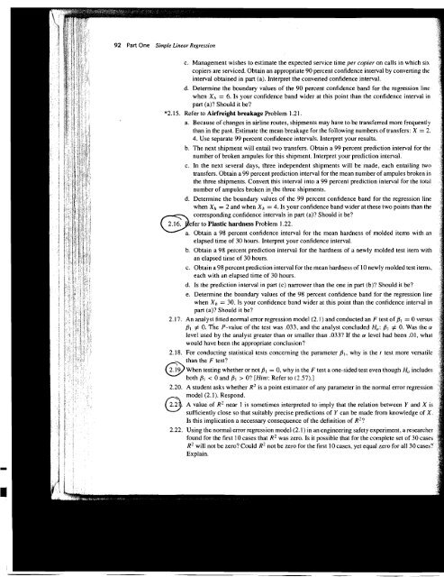
92 Part One Simple Linear Regression
c. Management wishes to estimate the expected service time per copier on calls in which six
copiers are serviced. Obtain an appropriate 90 percent confidence interval by converting the
interval obtained in part (a). lnterpret the converted confidence interval.
d. Determine the boundary values of the 90 percent confidence band for the regression line
when X,, = 6. Is your confidence band wider at this point than the confidence interval in
part (a)? Should it be?
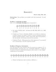
*2.15. Refer to Airfreight breakage Problem I .21.
a. Because of changes in airline routes, shipments may have to be transferred more frequently
than in the past. Estimate the mean breakage for the following numbers of transfers: X = 2.
4. Use separate 99 percent confidence intervals. Interpret your results.
b. The next shipment will entail two transfers. Obtain a 99 percent prediction interval for the
number of broken ampules for this shipment. lnterpret your prediction interval.
c. In the next several days, thee independent sh~pments will be made, each entailing two
transfers. Obtain a 99 percent prediction interval for the mean number of ampules broken in
the three shipments. Convert this interval into a 99 percent prediction interval for the total
number of ampules broken inJhe three shipments.
d. Determine the boundary values of the 99 percent confidence band for the regression line
when Xh = 2 and when Xh = 4. Is your confidence band wider at these two points than the
elapsed time of 30 hours. Interpret your confidence interval.
b. Obtain a 98 percent prediction interval for the hardness of a newly molded test item with
an elapsed time of 30 hours.
c. Obtain a 98 percent prediction interval for the mean hardness of 10 newly molded test items,
each with an elapsed time of 30 hours.
d. Is the prediction interval in part (c) narrower than the one in part (b)? Should it be?
e. Determine the boundary values of the 98 percent confidence band for the regression line
when Xh = 30. 1s your confidence band wider at this point than the confidence interval in
part (a)? Should it be?
2.17. An analyst fitted normal error regression model (2. I ) and conducted an F test of PI = 0 versus
PI # 0. he P-value of the test was .033, and the analyst concluded H,: PI # 0. Was the a
level used by the analyst greater than or smaller than .033? If the a level had been .Ol, whar
would have been the avvrovriate conclusion?
2.20. A student asks whether R' is a point estimator of any parameter in the normal error regression #
2.22. Using the normal error regression model (2.1) in an engineering safety experiment, a researcher
found for the first 10 cases that R' was zero. IS it possible that for the complete set of 30 cases
R2 will not be zero? Could R2 not be zero for the first 10 cases, yet equal zero for all 30 cases?
Explain.

3.23. Rel'er to Grade puint average Problem I. 19.
a. Set up the ANOVA tahlc.
Chapter 2 II!~~.I~,II

I
I
i
148 Part One Simple Linear Regression
d. Plot the residuals ei against Xi to ascertain whether any departures from regression
model (2.1) are evident. What is your conclusion?
e. Prepare a normal probability plot of the residuals. Also obtain the coefficient of correlation
between the ordered residuals and their expected values under normality to ascertain whether
the normality assumption is reasonable here. Use Table B.6 and a = .01. What do you
conclude?
f. Prepare a time plot of the residuals. What information is provided by your plot?
g. Assume that (3.10) is applicable and conduct the Breusch-Pagan test to determine whether
or not the error variance varies with the level of X. Use (Y = .lo. State the alternatives,
decision rule, and conclusion. Does your conclusion support your preliminary findings in
a. Obtain the residuals ei and prepare a box plot of the residuals. What information is provided
by your plot?
b. Plot the residuals ei against the fitted values pi to ascertain whether any departures from
regression model (2.1) are evident. State your findings.
c. Prepare a normal probability plot of the residuals. Also obtain the coefficient of correlation
between the ordered residuals and their expected values under normality. Does the normality
assumption appear to be reasonable here? Use Table B.6 and (Y = .05.
*3.7. Refer to Muscle mass Problem 1.27.
c. Plot the residuals e, against ?; and also against Xi on separate graphs to ascertain wh
any departures from regression model (2.1) are evident. Do the two plots provide the
information? State your conclusions.
d. Prepare a normal probability plot of the residuals. Also obtain the coefficient of correla
between the ordered residuals and their expected values under normality to ascertain whe
or not the error variance varies with the level of X. Use (Y = .01. State the alte
decision rule, and conclusion. Is your conclusion consistent with your preliminary
in part (c)?
3.8. Refer to Crime rate Problem 1.28.
a. Prepare a stem-and-leaf plot for the percentage of individuals in the county having at 1
a high school diploma Xi. What information does your plot provide?
b. Obtain the residuals ei and prepare a box plot of the residuals. Does the distribution of
residuals appear to be symmetrical?

150 Part One Simple Linear Regression
*3.13. Refer to Copier maintenance Problem.-I .20.
a. What are the alternative conclusions when testing for lack of fit of a linear regression
function?
b. Perform the test indicated in part (a). Control the risk of Type I error at .05. State the decision
rule and conclusion.
c. Does the test in part (b) detect other departures from regression model (2.1), such as lack
of constant variance or lack of normality in the error terms? Could the results of the test of
lack of fit be affected by such departures? Discuss.
3.14. Refer to PIastic hardness Problem 1.22.
a. Perform the F test to determine whether or not there is lack of fit of a linear regression
function; use cr = .01. State the alternatives, decision rule, and conclusion.
b. Is there any advantage of having an equal number of replications at each of the X levels? Is
there any disadvantage? .
c. Does the test in part (a) indicate what regression function is appropriate when it leads to the
conclusion that the regression function is not linear? How would you proceed?
3.15. Solution concentration. A chemist studied the concentration of a solution (Y) over time (X).
Fifteen identical solutions were prepared. The 15 solutions were randomly divided into five
sets of three, and the five sets were measured, respectively, after 1, 3, 5, 7, and 9 hours. The
results follow.
3 ... 13
Yi: .07 .09 .08 ... 2.84 2.57 3.10
a. Fit a linear regression function.
b. Perform the F test to determine whether or not there is lack of fit of a linear regression
function; use cr = .025. State the alternatives, decision rule, and conclusion.
c. Does the test in part (b) indicate what regression function is appropriate when it leads to the
conclusion that lack of fit of a linear regression function exists? Explain.
3.1 6. Refer to Solution concentration Problem 3.15.
a. Prepare a scatter plot of the data. What transformation of Y might you try, using the prototy
patterns in Figure 3.15 to achieve constant variance and linearity?
b. Use the Box-Cox procedure and standardization (3.36) to find an appropriate powe
transformation. Evaluate SSE for ,I = -.2, -. 1,0, .I, .2. What transformation of Y i
suggested?
c. Use the transformation Y' = log,, Y and obtain the estimated linear regression function
the transformed data.
d. Plot the estimated regression line and the transformed data. Does the regression line ap
to be a good fit to the transformed data?
e. Obtain the residuals and plot them against the fitted values. Also prepare a normal probabi
plot. What do your plots show?
f. Express the estimated regression function in the original units.
10 years ago. The data are as follows, where X is the year (coded) and Y is sales in thou

X,: 0 1 2 3 4 5 6 7 8 9
Y,: 98 135 162 178 221 232 283 300 374 395
:I. Prepare u scatter plot of the dnta. Does a linear relation appear adeq~~ate here?
b. Use the Box-Cox procedul- *id standardiz:~tion (3.36) to tind an appropriate power trnnsforination
of Y . Evaluate 4S.A or 1 = .3, .4. .5, .6. .7. What tfiuisformation of Y is suggested?
c. Use the t~.anstor~nation Y' = fi and obtain the estimatetl linenrregrcssion function for the
t~msformecl dam.
d. Plot the estimated ~.cgression line and the transformed data. Does the regression line appear
to be a good ti1 to the transformed data?
e. Obtain the residu:lls:uid plot them against the titted values. Also prepare anormnl probability
plot. What do yo~~r plots show'?
t'. Express the estimated regression function in the original units.
3.18. Production time. In ;I ~n;uiuh~cturing study, the procluction times l'or I I I recent production
runs were obtained. The table below lists forcach run the production time in IIOLII.S (Y) ;111d [he
production lot size (X ).
E Y,: 14.28 8.80 12.49 .. 16.37 11.45 15.78
X' = and obtain the estimated linear regression function for the (
b. Use the trnnsfor~natio~i
i . >..
trnnsfor~ned data. z:~.
c. Plot the estimated regression line and the transformed data. Does (lie regression line appear .
to be a good tit to thc transformed data? %
d. Obtain the residuals ;uid plot them against the fitted values. Also prepare :I normill probability
plot. What do your plots show?
e. Express the estimated regression function in the original ~~nits.
I I I-I.~ 3.19. A student ti tted a linear regression filnction for a class assignment. The student plotted the
residuals e, against Yj and found a positive relation. When the residuals were plotted against
the fitted values p;. the student found no relation. How could this difference arise? Which is
the more meaningful plot?
i.20. If the error terlns in a regression model are independent N(0, a'), what can be said about the
error terms after transformation X' = I / X is used? Is the situation the same after transformation
Y' = I/ Y is used?
;.?I. Derive the result in (3.29).
.;
j .;:
I i
i s i-~
+ .>.
: k::