CHAPTER 2 Univariate Time Series Models 2.1 Least ... - Statistics
CHAPTER 2 Univariate Time Series Models 2.1 Least ... - Statistics
CHAPTER 2 Univariate Time Series Models 2.1 Least ... - Statistics

Create successful ePaper yourself
Turn your PDF publications into a flip-book with our unique Google optimized e-Paper software.
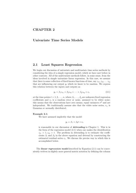
<strong>CHAPTER</strong> 2<br />
<strong>Univariate</strong> <strong>Time</strong> <strong>Series</strong> <strong>Models</strong><br />
<strong>2.1</strong> <strong>Least</strong> Squares Regression<br />
We begin our discussion of univariate and multivariate time series methods by<br />
considering the idea of a simple regression model, which we have met before in<br />
other contexts. All of the multivariate methods follow, in some sense, from the<br />
ideas involved in simple univariate linear regression. In this case, we assume<br />
that there is some collection of fixed known functions of time, say zt1, zt2, . . . ztq<br />
that are influencing our output yt which we know to be random. We express<br />
this relation between the inputs and outputs as<br />
yt = β1zt1 + β2zt2 + · · · + βqztq + et<br />
(<strong>2.1</strong>)<br />
at the time points t = 1, 2, . . . , n, where β1, . . . , βq are unknown fixed regression<br />
coefficients and et is a random error or noise, assumed to be white noise;<br />
this means that the observations have zero means, equal variances σ 2 and are<br />
independent. We traditionally assume also that the white noise series, et, is<br />
Gaussian or normally distributed.<br />
Example <strong>2.1</strong>:<br />
We have assumed implicitly that the model<br />
yt = β1 + β2t + et<br />
is reasonable in our discussion of detrending in Chapter 1. This is in<br />
the form of the regression model (<strong>2.1</strong>) when one makes the identification<br />
zt1 = 1, zt2 = t. The problem in detrending is to estimate the coefficients<br />
β1 and β2 in the above equation and detrend by constructing the<br />
estimated residual series et. We discuss the precise way in which this is<br />
accomplished below.<br />
The linear regresssion model described by Equation (<strong>2.1</strong>) can be conveniently<br />
written in slightly more general matrix notation by defining the column
<strong>2.1</strong>: <strong>Least</strong> Squares Regression 27<br />
vectors zt = (zt1, . . . , ztq) ′ and β = (β1, . . . , βq) ′ so that we write (<strong>2.1</strong>) in the<br />
alternate form<br />
yt = β ′ zt + et. (2.2)<br />
To find estimators for β and σ 2 it is natural to determine the coefficient vector<br />
β minimizing e 2 t with respect to β. This yields least squares or maximum<br />
likelihood estimator ˆ β and the maximum likelihood estimator for σ 2 which is<br />
proportional to the unbiased<br />
ˆσ 2 n−1<br />
1 <br />
=<br />
(yt −<br />
(n − q)<br />
ˆ β ′<br />
zt) 2<br />
t=0<br />
An alternate way of writing the model (2.2) is as<br />
(2.3)<br />
y = Zβ + e (2.4)<br />
where Z ′ = (z1, z2, . . . , zn) is a q×n matrix composed of the values of the input<br />
variables at the observed time points and y ′ = (y1, y2, . . . , yn) is the vector of<br />
observed outputs with the errors stacked in the vector e ′ = (e1, e2, . . . , en)<br />
.The ordinary least squares estimators ˆ β are the solutions to the normal<br />
equations<br />
Z ′ Z ˆ β = Z ′ y,<br />
You need not be concerned as to how the above equation is solved in practice<br />
as all computer packages have efficient software for inverting the q × q matrix<br />
Z ′ Z to obtain<br />
ˆβ = (Z ′ Z) −1 Z ′ y. (2.5)<br />
An important quantity that all software produces is a measure of uncertainty<br />
for the estimated regression coefficients, say<br />
cov{ ˆ ˆ β} = ˆσ 2 (Z ′ Z) −1 . (2.6)<br />
If cij denotes an element of C = (Z ′ Z) −1 , then cov( ˆ βi, ˆ βj) = σ 2 cij and a<br />
100(1 − α)% confidence interval for βi is<br />
ˆβi ± tn−q(α/2)ˆσ √ cii, (2.7)<br />
where tdf (α/2) denotes the upper 100(1 − α)% point on a t distribution with<br />
df degrees of freedom.<br />
Example 2.2:<br />
Consider estimating the possible global warming trend alluded to in Section<br />
1.1.2. The global temperature series, shown previously in Figure<br />
1.3 suggests the possibility of a gradually increasing average temperature<br />
over the 123 year period covered by the land-based series. If we<br />
fit the model in Example <strong>2.1</strong>, replacing t by t/100 to convert to a 100
28 1 <strong>Univariate</strong> <strong>Time</strong> <strong>Series</strong> <strong>Models</strong><br />
year base so that the increase will be in degrees per 100 years, we obtain<br />
ˆβ1 = 38.72, ˆ β2 = .9501 using (2.5). The error variance, from (2.3), is<br />
.0752, with q = 2 and n = 123. Then (2.6) yields<br />
cov( ˆ ˆ β1, ˆ β2) =<br />
1.8272 −.0941<br />
−.0941 .0048<br />
leading to an estimated standard error of √ .0048 = .0696. The value of t<br />
with n−q = 123−2 = 121 degrees of freedom for α = .025 is about 1.98,<br />
leading to a narrow confidence interval of .95 ± .138 for the slope leading<br />
to a confidence interval on the one hundred year increase of about .81<br />
to 1.09 degrees. We would conclude from this analysis that there is a<br />
substantial increase in global temperature amounting to an increase of<br />
roughly one degree F per 100 years.<br />
1<br />
0.5<br />
0<br />
Detrended Temperature<br />
ACF = γ x (h)<br />
−0.5<br />
0 5 10<br />
lag<br />
15 20<br />
1<br />
0.5<br />
0<br />
Differenced Temperature<br />
ACF = γ x (h)<br />
−0.5<br />
0 5 10<br />
lag<br />
15 20<br />
1<br />
0.5<br />
0<br />
<br />
,<br />
PACF = Φ hh<br />
−0.5<br />
0 5 10<br />
lag<br />
15 20<br />
1<br />
0.5<br />
0<br />
PACF = Φ hh<br />
−0.5<br />
0 5 10<br />
lag<br />
15 20<br />
Figure <strong>2.1</strong> Autocorrelation functions (ACF) and partial autocorrelation functions<br />
(PACF) for the detrended (top panel) and differenced (bottom panel) global<br />
temperature series.<br />
If the model is reasonable, the residuals êt = yt − ˆ β1 − ˆ β2 t should be<br />
essentially independent and identically distributed with no correlation evident.<br />
The plot that we have made in Figure 1.3 of the detrended global temperature<br />
series shows that this is probably not the case because of the long low frequency
<strong>2.1</strong>: <strong>Least</strong> Squares Regression 29<br />
in the observed residuals. However, the differenced series, also shown in Figure<br />
1.3 (second panel), appears to be more independent suggesting that perhaps<br />
the apparent global warming is more consistent with a long term swing in<br />
an underlying random walk than it is of a fixed 100 year trend. If we check<br />
the autocorrelation function of the regression residuals, shown here in Figure<br />
<strong>2.1</strong>, it is clear that the significant values at higher lags imply that there is<br />
significant correlation in the residuals. Such correlation can be important<br />
since the estimated standard errors of the coefficients under the assumption<br />
that the least squares residuals are uncorrelated is often too small. We can<br />
partially repair the damage caused by the correlated residuals by looking at a<br />
model with correlated errors. The procedure and techniques for dealing with<br />
correlated errors are based on the Autoregressive Moving Average (ARMA)<br />
models to be considered in the next sections. Another method of reducing<br />
correlation is to apply a first difference ∆xt = xt − xt−1 to the global trend<br />
data. The ACF of the differenced series, also shown in Figure <strong>2.1</strong>, seems to<br />
have lower correlations at the higher lags. Figure 1.3 shows qualitatively that<br />
this transformation also eliminates the trend in the original series.<br />
Since we have again made some rather arbitrary looking specifications for<br />
the configuration of dependent variables in the above regression examples, the<br />
reader may wonder how to select among various plausible models. We mention<br />
that two criteria which reward reducing the squared error and penalize for<br />
additional parameters are the Akaike Information Criterion<br />
AIC(K) = log ˆσ 2 + 2K<br />
n<br />
and the Schwarz Information Criterion<br />
SIC(K) = log ˆσ 2 +<br />
(2.8)<br />
K log n<br />
, (2.9)<br />
n<br />
(Schwarz, 1978) where K is the number of parameters fitted (exclusive of variance<br />
parameters) and ˆσ 2 is the maximum likelihood estimator for the variance.<br />
This is sometimes termed the Bayesian Information Criterion, BIC and will<br />
often yield models with fewer parameters than the other selection methods. A<br />
modification to AIC(K) that is particularly well suited for small samples was<br />
suggested by Hurvich and Tsai (1989). This is the corrected AIC, given by<br />
AICC(K) = log ˆσ 2 +<br />
n + K<br />
n − K − 2<br />
(<strong>2.1</strong>0)<br />
The rule for all three measures above is to choose the value of K leading to the<br />
smallest value of AIC(K) or SIC(K) or AICC(K). We will give an example<br />
later comparing the above simple least squares model with a model where the<br />
errors have a time series correlation structure.<br />
The organization of this chapter is patterned after the landmark approach<br />
to developing models for time series data pioneered by Box and Jenkins (see
30 1 <strong>Univariate</strong> <strong>Time</strong> <strong>Series</strong> <strong>Models</strong><br />
Box et al, 1994). This assumes that there will be a representation of time<br />
series data in terms of a difference equation that relates the current value<br />
to its past. Such models should be flexible enough to include non-stationary<br />
realizations like the random walk given above and seasonal behavior, where<br />
the current value is related to past values at multiples of an underlying season;<br />
a common one might be multiples of 12 months (1 year) for monthly data.<br />
The models are constructed from difference equations driven by random input<br />
shocks and are labeled in the most general formulation as ARIMA , i.e.,<br />
AutoRegressive Integrated Moving Average processes. The analogies<br />
with differential equations, which model many physical processes, are obvious.<br />
For clarity, we develop the separate components of the model sequentially,<br />
considering the integrated, autoregressive and moving average in order, followed<br />
by the seasonal modification. The Box-Jenkins approach suggests three<br />
steps in a procedure that they summarize as l identification, estimation<br />
and forecasting. Identification uses model selection techniques, combining<br />
the ACF and PACF as diagnostics with the versions of AIC given above to<br />
find a parsimonious (simple) model for the data. Estimation of parameters in<br />
the model will be the next step. Statistical techniques based on maximum likelihood<br />
and least squares are paramount for this stage and will only be sketched<br />
in this course. Finally, forecasting of time series based on the estimated parameters,<br />
with sensible estimates of uncertainty, is the bottom line, for any<br />
assumed model.<br />
2.2 Integrated (I) <strong>Models</strong><br />
We begin our study of time correlation by mentioning a simple model that will<br />
introduce strong correlations over time. This is the random walk model which<br />
defines the current value of the time series as just the immediately preceding<br />
value with additive noise. The model forms the basis, for example, of the<br />
random walk theory of stock price behavior. In this model we define<br />
xt = xt−1 + wt, (<strong>2.1</strong>1)<br />
where wt is a white noise series with mean zero and variance σ 2 . Figure 2.2<br />
shows a typical realization of such a series and we observe that it bears a<br />
passing resemblance to the global temperature series. Appealing to (<strong>2.1</strong>1),<br />
the best prediction of the current value would be expected to be given by its<br />
immediately preceding value. The model is, in a sense, unsatisfactory, because<br />
one would think that better results would be possible by a more efficient use<br />
of the past.<br />
The ACF of the original series, shown in Figure 2.3, exhibits a slow decay<br />
as lags increase. In order to model such a series without knowing that it is<br />
necessarily generated by (<strong>2.1</strong>1), one might try looking at a first difference and<br />
comparing the result to a white noise or completely independent process. It is
2.2 I <strong>Models</strong> 31<br />
5<br />
0<br />
−5<br />
−10<br />
Random walk: x t =x t−1 +w t<br />
−15<br />
0 20 40 60 80 100 120 140 160 180 200<br />
2<br />
1<br />
0<br />
−1<br />
−2<br />
3 First Difference: x t −x t−1<br />
−3<br />
0 20 40 60 80 100 120 140 160 180 200<br />
Figure 2.2 A typical realization of the random walk series (top panel and the first<br />
difference of the series (bottom panel)<br />
clear from (<strong>2.1</strong>1) that the first difference would be ∆xt = xt −xt−1 = wt which<br />
is just white noise. The ACF of the differenced process, in this case, would be<br />
expected to be zero at all lags h = 0 and the sample ACF should reflect this<br />
behavior. The first difference of the random walk in Figure 2.2 is also shown<br />
in Figure 2.3 and we note that it appears to be much more random. The ACF,<br />
shown in Figure 2.3, reflects this predicted behavior, with no significant values<br />
for lags other than zero. It is clear that (<strong>2.1</strong>1) is a reasonable model for this<br />
data. The original series is nonstationary, with an autocorrelation function<br />
that depends on time of the form<br />
⎧ <br />
⎪⎨<br />
t<br />
t+h , h ≥ 0<br />
ρ(xt+h, xt) =<br />
⎪⎩<br />
<br />
t+h<br />
t , h < 0
32 1 <strong>Univariate</strong> <strong>Time</strong> <strong>Series</strong> <strong>Models</strong><br />
1<br />
0.5<br />
0<br />
Random Walk<br />
ACF = γ x (h)<br />
−0.5<br />
0 5 10<br />
lag<br />
15 20<br />
1<br />
0.5<br />
0<br />
First Difference<br />
ACF = γ x (h)<br />
−0.5<br />
0 5 10<br />
lag<br />
15 20<br />
1<br />
0.5<br />
0<br />
PACF = Φ hh<br />
−0.5<br />
0 5 10<br />
lag<br />
15 20<br />
1<br />
0.5<br />
0<br />
PACF = Φ hh<br />
−0.5<br />
0 5 10<br />
lag<br />
15 20<br />
Figure 2.3 Autocorrelation functions (ACF) and partial autocorrelation functions<br />
(PACF) for the random walk (top panel) and the first difference (bottom<br />
panel) series.<br />
The above example, using a difference transformation to make a random<br />
walk stationary, shows a very particular case of the model identification procedure<br />
advocated by Box et al (1994). Namely, we seek a linearly filtered<br />
transformation of the original series, based strictly on the past values, that<br />
will reduce it to completely random white noise. This gives a model that<br />
enables prediction to be done with a residual noise that satisfies the usual<br />
statistical assumptions about model error.<br />
We will introduce, in the following discussion, more general versions of<br />
this simple model that are useful for modeling and forecasting series with<br />
observations that are correlated in time. The notation and terminology were<br />
introduced in the landmark work by Box and Jenkins (1970) (see Box et al,<br />
1994). A requirement for the ARMA model of Box and Jenkins is that the<br />
underlying process be stationary. Clearly the first difference of the random<br />
walk is stationary but the ACF of the first difference shows relatively little<br />
dependence on the past, meaning that the differenced process is not predictable<br />
in terms of its past behavior.<br />
To introduce a notation that has advantages for treating more general models,<br />
define the backshift operator B as the result of shifting the series back<br />
by one time unit, i.e.<br />
Bxt = xt−1, (<strong>2.1</strong>2)
2.2 AR <strong>Models</strong> 33<br />
and applying successively higher powers, B k xt = xt−k. The operator has many<br />
of the usual algebraic properties and allows, for example, writing the random<br />
walk model (<strong>2.1</strong>1) as<br />
(1 − B)xt = wt.<br />
Note that the difference operator discussed previously in 1.2.2 is just ∇ = 1−B.<br />
Identifying nonstationarity is an important first step in the Box-Jenkins<br />
procedure. From the above discussion, we note that the ACF of a nonstationary<br />
process will tend to decay rather slowly as a function of lag h. For example,<br />
a straightly line would be perfectly correlated, regardless of lag. Based on<br />
this observation, we mention the following properties that aid in identifying<br />
non-stationarity.<br />
Property P<strong>2.1</strong>: ACF and PACF of a non-stationary time series<br />
The ACF of a non-stationary time series decays very slowly as<br />
a function of lag h. The PACF of a non-stationary time series<br />
tends to have a peak very near unity at lag 1, with other values<br />
less than the significance level.<br />
2.3 Autoregressive (AR) <strong>Models</strong><br />
Now, extending the notions above to more general linear combinations of past<br />
values might suggest writing<br />
xt = φ1xt−1 + φ2xt−2 + . . . φpxt−p + wt<br />
(<strong>2.1</strong>3)<br />
as a function of p past values and an additive noise component wt. The model<br />
given by (<strong>2.1</strong>2) is called an autoregressive model of order p, since it is assumed<br />
that one needs p past values to predict xt. The coefficients φ1, φ2, . . . , φp<br />
are autoregressive coefficients, chosen to produce a good fit between the observed<br />
xt and its prediction based on xt−1, xt−2, . . . , xt−p. It is convenient to<br />
rewrite (<strong>2.1</strong>3), using the backshift operator, as<br />
where<br />
φ(B)xt = wt, (<strong>2.1</strong>4)<br />
φ(B) = 1 − φ1B − φ2B 2 − . . . − φpB p<br />
(<strong>2.1</strong>5)<br />
is a polynomial with roots (solutions of φ(B) = 0) outside the unit circle<br />
(|Bk| > 1). The restrictions are necessary for expressing the solution xt of<br />
(<strong>2.1</strong>4) in terms of present and past values of wt. That solution has the form<br />
xt = ψ(B)wt<br />
(<strong>2.1</strong>6)
34 1 <strong>Univariate</strong> <strong>Time</strong> <strong>Series</strong> <strong>Models</strong><br />
where<br />
ψ(B) =<br />
∞<br />
ψkB k , (<strong>2.1</strong>7)<br />
k=0<br />
is an infinite polynomial (ψ0 = 1), with coefficients determined by equating<br />
coefficients of B in<br />
ψ(B)φ(B) = 1. (<strong>2.1</strong>8)<br />
Equation (<strong>2.1</strong>6) can be obtained formally by noting that choosing ψ(B) satisfying<br />
(<strong>2.1</strong>8), and multiplying both sides of (<strong>2.1</strong>6) by ψ(B) gives the representation<br />
(<strong>2.1</strong>6). It is clear that the random walk has B1 = 1, which does not<br />
satisfy the restriction and the process is nonstationary.<br />
Example 2.2<br />
Suppose that we have an autoregressive model (<strong>2.1</strong>3) with p = 1, i.e.,<br />
xt − φ1xt−1 = (1 − φ1B)xt = wt. Then (<strong>2.1</strong>8) becomes<br />
(1 + ψ1B + ψ2B 2 + . . .)(1 − φ1B) = 1<br />
Equating coefficients of B implies that ψ1 − φ1 = 0 or ψ1 = φ1. For B 2 ,<br />
we would get ψ2 − φ1ψ1 = 0, or ψ2 = φ 2 1. Continuing, we obtain ψk = φ k 1<br />
and the representation is<br />
and we have<br />
ψ(B) = 1 +<br />
xt =<br />
∞<br />
k=0<br />
∞<br />
φ k 1B k<br />
k=1<br />
φ k 1wt−k. (<strong>2.1</strong>9)<br />
The representation (<strong>2.1</strong>6) is fundamental for developing approximate<br />
forecasts and also exhibits the series as a linear process of the form considered<br />
in Problem 1.4.<br />
For data involving such autoregressive (AR) models as defined above, the<br />
main selection problems are deciding that the autoregressive structure is appropriate<br />
and then in determining the value of p for the model. The ACF of<br />
the process is a potential aid for determining the order of the process as are<br />
the model selection measures (2.8)-(<strong>2.1</strong>0). To determine the ACF of the pth<br />
order AR in (<strong>2.1</strong>3), , write the equation as<br />
xt −<br />
p<br />
k=1<br />
φkxt−k = wt
2.2 AR <strong>Models</strong> 35<br />
and multiply both sides by xt−h, h = 1, 2, . . .. Assuming that the mean E(xt) =<br />
0, and using the definition of the autocovariance function (1.2) leads to the<br />
equation<br />
p<br />
E[(xt − φkxt−k)xt−h] = E[wtxt−h]<br />
k=1<br />
The left-hand side immediately becomes<br />
γx(h) −<br />
p<br />
φkγx(h − k).<br />
k=1<br />
The representation (<strong>2.1</strong>6) implies that<br />
E[wtxt−h] = E[wt(wt−h + ψ1wt−h−1 + ψ2wt−h−2 + . . .)]<br />
For h = 0, we get σ 2 w. For all other h, the fact that the wt are independent<br />
implies that the right-hand side will be zero. Hence, we may write the equations<br />
for determining γx(h) as<br />
and<br />
γx(0) −<br />
γx(h) −<br />
p<br />
φkγx(h − k) = σ 2 w<br />
k=1<br />
(2.20)<br />
p<br />
φkγx(h − k) = 0 (2.21)<br />
k=1<br />
for h = 1, 2, 3, . . .. Note that one will need the property γx(−h) = γx(h)<br />
in solving these equations. Equations (2.20) and (2.21) are called the Yule-<br />
Walker Equations (see Yule, 1927, Walker, 1931).<br />
Example 2.3<br />
Consider finding the ACF of the first-order autoregressive model. First,<br />
(2.21) implies that γx(0) − φ1γx(1) = σ 2 w. For h = 1, 2, . . ., we obtain<br />
γx(h) − φ1γx(h − 1) = 0 Solving these successively gives<br />
Combining with (2.20) yields<br />
γx(h) = γx(0)φ h 1<br />
γx(0) = σ2 w<br />
1 − φ 2 1<br />
It follows that the autocovariance function is<br />
γx(h) = σ2 w<br />
1 − φ2 φ<br />
1<br />
h 1
36 1 <strong>Univariate</strong> <strong>Time</strong> <strong>Series</strong> <strong>Models</strong><br />
Taking into account that γx(−h) = γx(h) and using (1.3), we obtain<br />
for h = 0, ±1, ±2, . . ..<br />
ρx(h) = φ |h|<br />
1<br />
The exponential decay is typical of autoregressive behavior and there may<br />
also be some periodic structure. However, the most effective diagnostic of AR<br />
structure is in the PACF and is summarized by the following identification<br />
property:<br />
Property P2.2: PACF for AR Process<br />
The partial autocorrelation function φhh as a function of lag h<br />
is zero for h > p, the order of the autoregressive process. This<br />
enables one to make a preliminary identification of the order p<br />
of the process using the partial autocorrelation function PACF.<br />
Simply choose the order beyond which most of the sample values<br />
of the PACF are approximately zero.<br />
To verify the above, note that the PACF (see Section 1.3.3) is basically the<br />
last cofficient obtained when minimizing the squared error<br />
MSE = E[(xt+h −<br />
h<br />
k=1<br />
akxt+h−k) 2 ].<br />
Setting the derivatives with respect to aj equal to zero leads to the equations<br />
This can be written as<br />
E[((xt+h −<br />
γx(j) −<br />
h<br />
akxt+h−k)xt+h−j] = 0<br />
k=1<br />
h<br />
akγx(j − k) = 0<br />
i=1<br />
for j = 1, 2, . . . , h. Now, from Equation and (2.21), it is clear that, for an<br />
AR(p), we may take ak = φk for k ≤ p and ak = 0 for k > p to get a solution<br />
for the above equation. This implies Property P2.3 above.<br />
Having decided on the order p of the model, it is clear that, for the estimation<br />
step, one may write the model (<strong>2.1</strong>3) in the regression form<br />
xt = φ ′ zt + wt, (2.22)
2.2 AR <strong>Models</strong> 37<br />
where φ = (φ1, φ2, . . . , φp) ′ corresponds to β and zt = (xt−1, xt−2, . . . , xt−p) ′<br />
is the vector of dependent variables in (2.2). Taking into account the fact that<br />
xt is not observed for t ≤ 0, we may run the regression approach in Section 3.1<br />
for t = p, p + 1, . . . , n − 1 to get estimators for φ and for σ 2 , the variance of the<br />
white noise process. These so-called conditional maximum likelihood estimators<br />
are commonly used because the exact maximum likelihood estimators involve<br />
solving nonlinear equations.<br />
Example 2.4<br />
We consider the simple problem of modeling the recruit series shown in<br />
Figure 1.1 using an autoregressive model. The bottom panel of Figure 1.9<br />
shows the autocorrelation ACF and partial autocorelation PACF functions<br />
of the recruit series. The PACF has large values for h = 1, 2 and<br />
then is essentially zero for higher order lags. This implies by Property<br />
P2.2 above that a second order (p = 2) AR model might provide a good<br />
fit. Running the regression program for the model<br />
leads to the estimators<br />
xt = β0 + φ1xt−1 + φ2xt−2 + wt<br />
ˆβ0 = 6.74(1.11), ˆ φ1 = 1.35(.04), ˆ φ2 = −.46(.04), ˆσ 2 = 90.31<br />
where the estimated standard deviations are in parentheses. To determine<br />
whether the above order is the best choice, we fitted models for<br />
p = 1, . . . , 10, obtaining corrected AICC values of 5.75, 5.52, 5.53, 5.54,<br />
5.54, 5.55, 5.55, 5.56, 5.57, and 5.58 respectively using (<strong>2.1</strong>0) with K = 2.<br />
This shows that the minimum AICC obtains for p = 2 and we choose<br />
the second-order model.<br />
Example 2.5<br />
The previous example used various autoregressive models for the recruits<br />
series, fitting a second-order regression model. We may also use this regression<br />
idea to fit the model to other series such as a detrended version<br />
of the Southern Oscillation Index (SOI) given in previous discussions.<br />
We have noted in our discussion of Figure 1.9 from the partial autocorrelation<br />
function (PACF) that a plausible model for this series might be<br />
a first order autoregression of the form given above with p = 1. Again,<br />
putting the model above into the regression framework (2.2) for a single<br />
coefficient leads to the estimators ˆ φ1 = .59 with standard error .04,<br />
ˆσ 2 = .09218 and AICC(1) = −1.375. The ACF of these residuals (not<br />
shown), however, will still show cyclical variation and it is clear that<br />
they still have a number of values exceeding the ±1.96/ √ n threshold
38 1 <strong>Univariate</strong> <strong>Time</strong> <strong>Series</strong> <strong>Models</strong><br />
(see Equation 1.14). A suggested procedure is to try higher order autoregressive<br />
models and successive models for p = 1, 2, . . . , 30 were fitted<br />
and the AICC(K) values are plotted in Figure 3.10 of Chapter 3 so we do<br />
not repeat it here. There is a clear minimum for a p = 16th order model.<br />
The coefficient vector is ˆ φ with components .40, .07, .15, .08, -.04, -.08,<br />
-.09, -.08, .00, .11, .16, .15, .03, -.20, -.14 and -.06 and ˆσ 2 = .07354.<br />
Finally, we give a general approach to forecasting for any process that can<br />
be written in the form (<strong>2.1</strong>6). This includes the AR, MA and ARMA processes.<br />
We begin by defining an h-step forecast of the process xt as<br />
x t t+h = E[xt+h|xt, xt−1, . . .] (2.23)<br />
Note that this is not exactly right because we only have x1, xt, . . . , xt available,<br />
so that conditioning on the infinite past is only an approximation. From this<br />
definition is reasonable to intuit that x t s = xt, s ≤ t and<br />
for s ≤ t. For s > t, use x t s and<br />
E[ws|xt, xt−1, . . .] = E[ws|wt, wt−1 . . .] = ws, (2.24)<br />
E[ws|xt, xt−1, . . .] = E[ws|wt, wt−1, . . .] = E[ws] = 0, (2.25)<br />
since ws will be independent of past values of wt. We define the h-step forecast<br />
variance as<br />
P t t+h = E[(xt+h − x t t+h) 2 |xt, xt−1, . . .]. (2.26)<br />
To develop an expression for this mean square error, note that, with ψ0 = 1,<br />
we can write<br />
∞<br />
xt+h = ψkwt+h−k.<br />
Then, since w t t+h−k<br />
so that the residual is<br />
k=0<br />
= 0 for t + h − k > t, i.e. k < h, we have<br />
x t t+h =<br />
∞<br />
k=h<br />
xt+h − x t h−1 <br />
t+h =<br />
ψkwt+h−k,<br />
k=0<br />
ψkwt+h−k,<br />
Hence, the mean square error (2.26) is just the variance of a linear combination<br />
of independent zero mean errors, with common variance σ 2 w<br />
h−1 <br />
P t t+h = σ 2 w ψ<br />
k=0<br />
2 k<br />
(2.27)
2.2 AR <strong>Models</strong> 39<br />
As an example, we consider forecasting the second order model developed for<br />
the recruit series in Example 2.5.<br />
Example 2.6<br />
Consider the one-step forecast x t t+1 first. Writing the defining equation<br />
for t + 1 gives<br />
xt+1 = φ1xt + φ2xt−1 + wt+1,<br />
so that<br />
x t t+1<br />
Continuing in this vein, we obtain<br />
Then,<br />
x t t+h<br />
x t t+2<br />
= φ1x t t + φ2x t t−1 + w t t+1<br />
= φ1xt + φ2xt−1 + 0<br />
= φ1x t t+1 + φ2x t t + w t t+2<br />
= φ1x t t+1 + φ2xt + 0.<br />
= φ1x t t+h−1 + φ2x t t+h−2 + wt t+h<br />
= φ1x t t+h−1 + φ2x t t+h−2<br />
for h > 2. Forecasts out to lag h = 4 and beyond, if necessary, can be<br />
found by solving (<strong>2.1</strong>8) for ψ1, ψ2 and ψ3, and substituting into (2.26).<br />
By equating coefficients of B, B 2 and B 3 in<br />
+ 0<br />
(1 − φ1B − φ2B 2 )(1 + ψ1B + ψ2B 2 + ψ3B 3 + . . .) = 1,<br />
we obtain ψ1 = φ1, ψ2 − φ2 + φ1ψ1 = 0 and ψ3 − φ1ψ2 − φ2ψ1 = 0.<br />
This gives the coefficients ψ1 = φ1, ψ2 = φ2 − φ 2 1, ψ3 = 2φ2φ1 − φ 2 1 From<br />
Example 2.5, we have ˆ φ1 = 1.35, ˆ φ2 = −.46, ˆσ 2 w = 90.31 and ˆ β0 = 6.74.<br />
The forecasts are of the form<br />
x t t+h = 6.74 + 1.35x t t+h−1 − .46x t t+h−2<br />
For the forecast variance, we evaluate ψ1 = 1.35, ψ2 = −2.282, ψ3 =<br />
−3.065, leading to 90.31, 90.31(2.288), 90.31(7.495) and 90.31(16.890) for<br />
forecasts at h = 1, 2, 3, 4. The standard deviations of the forecasts are<br />
9.50, 14.37, 26.02 and 39.06 for the standard errors of the forecasts. The<br />
recruit series values range from 20 to 100 so the forecast uncertainty will<br />
be rather large.
40 1 <strong>Univariate</strong> <strong>Time</strong> <strong>Series</strong> <strong>Models</strong><br />
2.4 Moving Average (MA) <strong>Models</strong><br />
We may also consider processes that contain linear combinations of underlying<br />
unobserved shocks, say, represented by white noise series wt. These moving<br />
average components generate a series of the form<br />
xt = wt − θ1wt−1 − θ2wt−2 − . . . − θqwt−q<br />
(2.28)<br />
where q denotes the order of the moving average component and θ1, θ2, . . . , θq<br />
are parameters to be estimated. Using the shift notation, the above equation<br />
can be written in the form<br />
xt = θ(B)wt<br />
(2.29)<br />
where<br />
θ(B) = 1 − θ1B − θ2B 2 − . . . − θqB q<br />
(2.30)<br />
is another polynomial in the shift operator B. It should be noted that the MA<br />
process of order q is a linear process of the form considered earlier in Problem<br />
1.4 with ψ0 = 1, ψ2 = −θ1, . . . , ψq = θq. This implies that the ACF will be<br />
zero for lags larger than q because terms in the form of the covariance function<br />
given in Problem 1.4 of Chapter 1 will all be zero. Specifically, he exact forms<br />
are<br />
for h + 0 and<br />
γx(0) = σ 2 w<br />
γx(h) = σ 2 w<br />
<br />
1 +<br />
q<br />
k=1<br />
q−h <br />
−θh +<br />
k=1<br />
θ 2 k<br />
<br />
θk+hθk<br />
for h = 1, . . . , q − 1, with γx(q) = −σ 2 wθq, and γx(h) = 0 for h > q.<br />
Hence, we will have<br />
<br />
(2.31)<br />
(2.32)<br />
P2.3: ACF for MA <strong>Series</strong><br />
For a moving average series of order q, note that the autocorrelation<br />
function (ACF) is zero for lags h > q, i.e. ρx(h) = 0<br />
for h > q. Such a result enables us to diagnose the order of a<br />
moving average component by examining ˆρx(h) and choosing q<br />
as the value beyond which the coefficients are essentially zero.<br />
Example 2.7<br />
Consider the varve thicknesses in Figure 1.10, which is described in Problem<br />
1.7 of Chapter 1. Figure 2.4 shows the ACF and PACF of the original<br />
log-transformed varve series and the first differences. The ACF of the<br />
original series indicates a possible non-stationary behavior, and suggests<br />
taking a first difference, interpreted hear as the percentage yearly change
2.2 MA <strong>Models</strong> 41<br />
in deposition. The ACF of the first difference shows a clear peak at h = 1<br />
and no other significant peaks, suggesting a first-order moving average.<br />
Fitting the first order moving average model xt = wt − θ1wt−1 to this<br />
data using the Gauss-Newton procedure described next leads to ˆ θ1 = .77<br />
and ˆσ 2 w = .2358.<br />
1<br />
0.5<br />
0<br />
log varves<br />
−0.5<br />
0 10 20 30<br />
1<br />
0.5<br />
0<br />
ACF<br />
First difference<br />
−0.5<br />
0 10 20 30<br />
1<br />
0.5<br />
0<br />
−0.5<br />
0 10 20 30<br />
1<br />
0.5<br />
0<br />
PACF<br />
−0.5<br />
0 10 20 30<br />
Figure 2.4 Autocorrelation functions (ACF) and partial autocorrelation functions<br />
(PACF) for the log varve series (top panel) and the first difference (bottom<br />
panel), showing a peak in the ACF at lag h = 1.<br />
Fitting the pure moving average term turns into a nonlinear problem as we<br />
can see by noting that either maximum likelihood or regression involves solving<br />
(2.28) or (2.29) for wt, and minimizing the sum of the squared errors. Suppose<br />
that the roots of π(B) = 0 are all outside the unit circle, then this is possible<br />
by solving π(B)θ(B) = 1, so that, for the vector parameter θ = (θ1, . . . , θq) ′ ,<br />
we may write<br />
wt(θ) = π(B)xt<br />
(2.33)<br />
and minimize<br />
SSE(θ) =<br />
n<br />
t=q+1<br />
w 2 t (θ)<br />
as a function of the vector parameter θ. We don’t really need to find the operator<br />
π(B) but can simply solve (2.23) recursively for wt, with w1, w2, . . . wq = 0
42 1 <strong>Univariate</strong> <strong>Time</strong> <strong>Series</strong> <strong>Models</strong><br />
and<br />
wt(θ) = xt +<br />
q<br />
k=1<br />
θkwt−k<br />
for t = q+1, . . . , n. It is easy to verify that SSE(θ) will be a nonlinear function<br />
of θ1, θ2, . . . , θq. However, note that<br />
′<br />
∂wt<br />
wt(θ) ≈ wt(θ0) + (θ − θ0),<br />
∂t<br />
where the derivative is evaluated at the previous guess θ0. Rearranging the<br />
above equation leads to<br />
<br />
wt(θ0) ≈ − ∂wt<br />
′<br />
(θ − θ0) + wt(θ), (2.34)<br />
∂θ<br />
which is just the regression model (2.2). Hence, we can begin with an initial<br />
guess θ0 = (.1, .1, . . . , .1) ′ , say and successively minimize SSE(θ) until<br />
convergence.<br />
In order to forecast a moving average series, note that<br />
q<br />
xt+h = wt+h − θkwt+h−k.<br />
The results below (2.24) imply that<br />
x t t+h = −<br />
q<br />
k=1<br />
k=h+1<br />
θkw t t+h−k,<br />
where the wt values needed for the above are computed recursively as before.<br />
Because of (<strong>2.1</strong>7), it is clear that ψ0 = 1 and ψk = −θk, k = 1, 2, . . . , q and<br />
these values can be substituted directly into the variance formula (2.27).<br />
2.5 Autoregressive Integrated Moving Average<br />
(ARIMA) <strong>Models</strong><br />
Now combining the autoregressive and moving average components leads<br />
to the autoregressive moving average ARMA(p, q) model, written as<br />
φ(B)xt = θ(B)wt, (2.35)<br />
where the polynomials in B are as defined earlier in (<strong>2.1</strong>5) and (2.29), with p<br />
autoregressive coefficients and q moving average coefficients. In the difference<br />
equation form, this becomes<br />
p<br />
q<br />
xt − φkxt−k = wt − θkwt−k. (2.36)<br />
k=1<br />
k=1
2.5 ARIMA <strong>Models</strong> 43<br />
The mixed processes do not satisfy the properties P<strong>2.1</strong>-P2.3 any more but<br />
they tend to behave in approximately the same way, even for the mixed cases.<br />
Estimation and forecasting for such problems are treated in essentially the<br />
same manner as for the AR and MA processes. We note that we can formally<br />
divide both sides of (2.25) by φ(B) and note that the usual representation<br />
(<strong>2.1</strong>6) holds when<br />
ψ(B)φ(B) = θ(B). (2.37)<br />
For forecasting, we determine the ψ1, ψ2, . . . by equating coefficients of B, B 2 , B 3 , . . .<br />
in (2.37), as before, assuming the all the roots of φ(B) = 0 are greater than<br />
one in absolute value. Similarly, we can always solve for the residuals, say<br />
wt = xt −<br />
p<br />
φkxt−k +<br />
k=1<br />
q<br />
k=1<br />
θkwt−k<br />
to get the terms needed for forecasting and estimation.<br />
(2.38)<br />
Example 2.8<br />
Consider the above mixed process with p = q = 1, i.e. ARMA(1, 1). By<br />
(2.26), we may write<br />
Now,<br />
so that<br />
xt = φ1xt−1 + wt − θ1wt−1.<br />
xt+1 = φ1xt + wt+1 − θ1wt<br />
x t t+1 = φ1xt + 0 − θ1wt<br />
and xt t+h = φxt t+h−1 for h > 1, leading to very simple forecasts in this<br />
case. Equating coefficients of Bk in<br />
leads to<br />
(1 − φB)(1 + ψ1B + ψ2B 2 + . . .) = (1 − θ1B)<br />
ψk = (φ1 − θ1)φ k−1<br />
1<br />
for k = 1, 2, . . .. Using (2.26) leads to the expression<br />
P t t+h<br />
= σ 2 w<br />
for the forecast variance.<br />
<br />
1 + (φ1 − θ1) 2 h−1 k=1 φ2(k−1)<br />
<br />
1<br />
<br />
<br />
= σ2 w 1 + (φ1−θ1) 2 (1−φ 2(h−1)<br />
1 )<br />
(1−φ2 1 )
44 1 <strong>Univariate</strong> <strong>Time</strong> <strong>Series</strong> <strong>Models</strong><br />
In the first example of this chapter, it was noted that nonstationary processes<br />
are characterized by a slow decay in the ACF as in Figure 2.3. In many of the<br />
cases where slow decay is present, the use of a first order difference<br />
∆xt = xt − xt−1<br />
= (1 − B)xt<br />
will reduce the nonstationary process xt to a stationary series ∆xt. On can<br />
check to see whether the slow decay has been eliminated in the ACF of the<br />
transformed series. Higher order differences, ∆ d xt = ∆∆ d−1 xt are possible<br />
and we call the process obtained when the d th difference is an ARMA series<br />
an ARIMA(p, d, q) series where p is the order of the autoregressive component,<br />
d is the order of differencing needed and q is the order of the moving average<br />
component. Symbolically, the form is<br />
φ(B)∆ d xt = θ(B)wt<br />
(2.39)<br />
The principles of model selection for ARIMA(p, d, q) series are obtained using<br />
the extensions of (2.8)-(<strong>2.1</strong>0) which replace K by K = p + q the total number<br />
of ARMA parameters.<br />
2.6 Seasonal ARIMA <strong>Models</strong><br />
When the autoregressive, differencing, or seasonal moving average behavior<br />
seems to occur at multiples of some underlying period s, a seasonal ARIMA<br />
series may result. The seasonal nonstationarity is characterized by slow decay<br />
at multiples of s and can often be eliminated by a seasonal differencing operator<br />
of the form<br />
∇ D s xt = (1 − B s ) D xt.<br />
For example, when we have monthly data, it is reasonable that a yearly phenomenon<br />
will induce s = 12 and the ACF will be characterized by slowly<br />
decaying spikes at 12, 24, 36, 48, . . . and we can obtain a stationary series by<br />
transforming with the operator (1−B 12 )xt = xt −xt−12 which is the difference<br />
between the current month and the value one year or 12 months ago.<br />
If the autoregressive or moving average behavior is seasonal at period s, we<br />
define formally the operators<br />
and<br />
Φ(B s ) = 1 − Φ1(B s ) − Φ2(B 2s ) − . . . − ΦP (B P s ) (2.40)<br />
Θ(B s ) = 1 − Θ1(B s ) − Θ2(B 2s ) − . . . − ΘQ(B Qs ). (2.41)<br />
The final form of the ARIMA(p, d, q) × ARIMA(P, D, Q)s model is<br />
Φ(B s )φ(B)∆ s D∆ d xt = Θ(B s )θ(B)wt<br />
(2.42)
2.5 SARIMA <strong>Models</strong> 45<br />
We may also note the properties below corresponding to P<strong>2.1</strong>-P2.3<br />
Property P<strong>2.1</strong>’: ACF and PACF of a seasonally non-stationary time<br />
series<br />
The ACF of a seasonally non-stationary time series decays<br />
very slowly at lag multiples s, 2s, 3s, . . . with zeros in between,<br />
where s denotes a seasonal period ,usually 12. The PACF of a<br />
non-stationary time series tends to have a peak very near unity<br />
at lag s.<br />
Property P2.2’: PACF for Seasonal AR <strong>Series</strong><br />
The partial autocorrelation function φhh as a function of lag<br />
h has nonzero values at s, 2s, 3s, . . . , P s, with zeros in between,<br />
and is zero for h > P s, the order of the seasonal autoregressive<br />
process. There should be some exponential decay.<br />
P2.3’: ACF for a Seasonal MA <strong>Series</strong><br />
For a seasonal moving average series of order Q, note that the<br />
autocorrelation function (ACF) has nonzero values at s, 2s, 3s, . . . , Qs<br />
and is zero for h > Qs<br />
Example 2.9:<br />
We illustrate by fitting the monthly birth series from 1948-1979 shown in<br />
Figure 2.5. The period encompasses the boom that followed the Second<br />
World War and there is the expected rise which persists for about 13<br />
years followed by a decline to around 1974, The series appears to have<br />
long-term swings, with seasonal effects super-imposed. The long-term<br />
swings indicate possible non-stationarity and we verify that this is the<br />
case by checking the ACF and PACF shown in the top panel of Figure<br />
2.6. Note, that by Property <strong>2.1</strong>, slow decay of the ACF indicates nonstationarity<br />
and we respond by taking a first difference. The results<br />
shown in the second panel of Figure 2.5 indicate that the first difference<br />
has eliminated the strong low frequency swing. The ACF, shown in the<br />
second panel from the top in Figure 2.6 shows peaks at 12, 24, 36, 48,<br />
..., with now decay. This behavior implies seasonal non-stationarity, by<br />
Property P<strong>2.1</strong>’ above, with s = 12. A seasonal difference of the first<br />
difference generates an ACF and PACF in Figure 2.6 that we expect for<br />
stationary series.<br />
Taking the seasonal difference of the first difference gives a series that<br />
looks stationary and has an ACF with peaks at 1 and 12 and a PACF with<br />
a substantial peak at 12 and lesser peaks at 12,24, .... This suggests trying<br />
either a first order moving average term, by Property P2.3, or a first order
46 1 <strong>Univariate</strong> <strong>Time</strong> <strong>Series</strong> <strong>Models</strong><br />
400<br />
300<br />
200<br />
50<br />
0<br />
−50<br />
50<br />
0<br />
−50<br />
50<br />
0<br />
−50<br />
Births<br />
50 100 150 200 250 300 350<br />
1st diff.<br />
50 100 150 200 250 300 350<br />
ARIMA(0,1,0)X(0,1,0) 12<br />
50 100 150 200 250 300 350<br />
ARIMA(0,1,1)X(0,1,1) 12<br />
50 100 150 200 250 300 350<br />
month<br />
Figure 2.5 Number of live births 1948(1)-1979(1) and residuals from models with a<br />
first difference, a first difference and a seasonal difference of order 12 and a<br />
fitted ARIMA(0, 1, 1) × (0, 1, 1)12 model.
2.5 SARIMA <strong>Models</strong> 47<br />
1<br />
0.5<br />
0<br />
−0.5<br />
0 20 40 60<br />
1<br />
0.5<br />
0<br />
−0.5<br />
0 20 40 60<br />
1<br />
0.5<br />
0<br />
−0.5<br />
0 20 40 60<br />
1<br />
0.5<br />
0<br />
−0.5<br />
0 20 40 60<br />
1<br />
0.5<br />
0<br />
ACF<br />
−0.5<br />
0 20 40 60<br />
lag lag<br />
1<br />
0.5<br />
0<br />
PACF<br />
data<br />
−0.5<br />
0 20 40 60<br />
1<br />
0.5<br />
0<br />
ARIMA(0,1,0)<br />
−0.5<br />
0 20 40 60<br />
1<br />
0.5<br />
0<br />
ARIMA(0,1,0)X(0,1,0) 12<br />
−0.5<br />
0 20 40 60<br />
1<br />
0.5<br />
0<br />
ARIMA(0,1,0)X(0,1,1) 12<br />
−0.5<br />
0 20 40 60<br />
1<br />
0.5<br />
0<br />
ARIMA(0,1,1)X(0,1,1) 12<br />
−0.5<br />
0 20 40 60<br />
Figure 2.6 Autocorrelation functions (ACF) and partial autocorrelation functions<br />
(PACF) for the birth series (top two panels), the first difference (second<br />
two panels) an ARIMA(0, 1, 0 × (0, 1, 1)12 model (third two panels) and an<br />
ARIMA(0, 1, 1) × (0, 1, 1)12 model (last two panels.<br />
seasonal moving average term with s = 12, by Property P2.3’ above. We<br />
choose to eliminate the largest peak first by applying a first-order seasonal<br />
moving average model with s = 12. The ACF and PACF of the residual<br />
series from this model, i.e. from ARIMA(0, 1, 0) × (0, 1, 112, written as<br />
(1 − B)(1 − B 12 )xt = (1 − Θ1B 12 )wt,
48 1 <strong>Univariate</strong> <strong>Time</strong> <strong>Series</strong> <strong>Models</strong><br />
Forecast 1979(2)−1982(1)<br />
450<br />
400<br />
350<br />
300<br />
250<br />
200<br />
lower 95%<br />
forecast<br />
upper 95%<br />
150<br />
370 375 380 385 390<br />
month<br />
395 400 405 410<br />
Figure 2.7 A 36 month forecast for the birth series with 95% uncertainty limits.<br />
is shown in the fourth panel from the top in Figure 2.6. We note that<br />
the peak at lag one is still there, with attending exponential decay in<br />
the PACF. This can be eliminated by fitting a first-order moving average<br />
term and we consider the model ARIMA(0, 1, 1) × (0, 1, 1)12, written as<br />
(1 − B)(1 − B 12 )xt = (1 − θ1B)(1 − Θ1B 12 )wt<br />
The ACF of the residuals from this model are relatively well behaved<br />
with a number of peaks either near or exceeding the 95% test of no<br />
correlation. Fitting this final ARIMA(0, 1, 1) × (0, 1, 1)12 model leads to<br />
the model<br />
(1 − B)(1 − B 12 )xt = (1 − .4896B)(1 − .6844B 12 )wt<br />
AICc = 4.95, R 2 = .9804 2 = .961, P − values = .000, .000<br />
R 2 is computed from saving the predicted values and then plotting against<br />
the observed values using the 2-D plot option. The format that ASTSA<br />
puts out these results is shown below.<br />
ARIMA(0,1,1)x(0,1,1)x12 from U.S. Births AICc = 4.94684 variance =<br />
51.1906 d.f. = 358 Start values = .1
2.5 SARIMA <strong>Models</strong> 49<br />
predictor coef st. error t-ratio p-value<br />
MA(1) .4896 .04620 10.5966 .000<br />
SMA(1) .6844 .04013 17.0541 .000<br />
(D1) (D(12)1) x(t) = (1 -.49B1) (1 -.68B12) w(t)<br />
The ARIMA search in ASTSA leads to the model<br />
(1−.0578B 12 )(1−B)(1−B 12 )xt = (1−.4119B−.1515B 2 )(1−.8136B 12 )wt<br />
with AICc = 4.8526, somewhat lower than the previous model. The seasonal<br />
autoregressive coefficient is not statistically significant and should<br />
probably be omitted from the model. The new model becomes<br />
(1 − B)(1 − B 12 )xt = (1 − .4088B − .1645B 2 )(1 − .6990B 12 )wt,<br />
yielding AICc = 4.92 and R 2 = .981 2 = .962, slightly better than the<br />
ARIMA(0, 1, 1) × (0, 1, 1)12 model. Evaluating these latter models leads<br />
to the conclusion that the extra parameters do not add a practically<br />
substantial amount to the predictability.<br />
The model is expanded as<br />
so that<br />
or<br />
(1 − B)(1 − B 12 )xt = (1 − θ1B)(1 − Θ1B 12 )wt<br />
(1 − B − B 12 + B 13 )xt = (1 − θ1B − θ1B 12 + θ1Θ1B 13 )wt<br />
xt − xt−1 − xt−12 + xt−13 = wt − θ1wt−1 − Θ1wt−12 + θ1Θ1wt−13<br />
xt = xt−1 + xt−12 − xt−13 + wt − θ1wt−1 − Θ1wt−12 + θ1Θ1wt−13<br />
The forecast is<br />
x t t+1 = xt + xt−11 − xt−12 − θ1wt − Θ1wt−11 + θ1Θ1wt−12<br />
x t t+2 = x t t+1 + xt−10 − xt−11 − Θ1wt−10 + θ1Θ1wt−11<br />
Continuing in the same manner, we obtain<br />
x t t+12 = x t t+11 + xt − xt−1 − Θ1wt + θ1Θ1wt−1<br />
for the 12 month forecast.
50 1 <strong>Univariate</strong> <strong>Time</strong> <strong>Series</strong> <strong>Models</strong><br />
The forecast limits are quite variable with a standard error that rises to<br />
20% of the mean by the end of the forecast period The plot shows that<br />
the general trend is upward, rising from about 250,000 to about 290,000<br />
births per year. One could check the actual records from the years 1979-<br />
1982. The direction is not certain because of the large uncertainty. One<br />
could compute the probability<br />
<br />
250 − 290<br />
P (Bt+47 ≤ 250, 000) = Φ<br />
= .25,<br />
60<br />
so there is a 75% chance of increase.<br />
A website where the forecasts can be compared on a yearly basis is<br />
http://www.cdc.gov/nccdphp/drh/pdf/nvs/nvs48 tb1.pdf<br />
Example <strong>2.1</strong>0:<br />
Figure 2.8 shows the autocorrelation function of the log-transformed J&J<br />
earnings series that is plotted in Figure 1.4 and we note the slow decay<br />
indicating the nonstationarity which has already been obvious in the<br />
Chapter 1 discussion. We may also compare the ACF with that of a<br />
random walk, shown in Figure 3.2, and note the close similarity. The<br />
partial autocorrelation function is very high at lag one which, under ordinary<br />
circumstances, would indicate a first order autoregressive AR(1,0)<br />
model, except that, in this case, the value is close to unity, indicating a<br />
root close to 1 on the unit circle. The only question would be whether<br />
differencing or detrending is the better transformation to stationarity.<br />
Following in the Box-Jenkins tradition, differencing leads to the ACF<br />
and PACF shown in the second panel and no simple structure is apparent.<br />
To force a next step, we interpret the peaks at 4, 8, 12, 16, . . . as<br />
contributing to a possible seasonal autoregressive term, leading to a possible<br />
ARIMA(0, 1, 0)×(1, 0, 0)4 and we simply fit this model and look at<br />
the ACF and PACF of the residuals, shown in the third two panels. The<br />
fit improves somewhat, with significant peaks still remaining at lag 1 in<br />
both the ACF and PACF. The peak in the ACF seems more isolated and<br />
there remains some exponentially decaying behavior in the PACF, so we<br />
try a model with a first-order moving average. The bottom two panels<br />
show the ACF and PACF of the resulting ARIMA(0, 1, 1) × (1, 0, 0)4<br />
and we note only relatively minor excursions above and below the 95%<br />
intervals under the assumption that the theoretical ACF is white noise.<br />
The final model suggested is (yt = log x2)<br />
(1 − Φ1B 4 )(1 − B)yt = (1 − θ1B)wt,<br />
where ˆ Φ1 = .820(.058), ˆ θ1 = .508(.098) and ˆσ 2 w = .0086. The model can<br />
be written in forecast form as<br />
yt = yt−1 + Φ1(yt−4 − yt−5) + wt − θ1wt−1.
2.6 Correlated Regression 51<br />
To forecast the original series for, say 4 quarters, we compute the forecast<br />
limits for yt = log xt and then exponentiate, i.e.<br />
x t t+h = exp{y t t+h}<br />
We note the large limits on the forecast values in Figure 2.9 and mention<br />
that the situation can be improved by the regression approach in the<br />
next section<br />
2.7 Regression <strong>Models</strong> With Correlated Errors<br />
The standard method for dealing with correlated errors et in the in the regression<br />
model<br />
yt = β ′ zt + et<br />
(2.2) ′<br />
is to try to transform the errors et into uncorrelated ones and then apply the<br />
standard least squares approach to the transformed observations. For example,<br />
let P be an n × n matrix that transforms the vector e = (e1, . . . , en) ′ into a<br />
set of independent identically distributed variables with variance σ 2 . Then,<br />
transform the matrix version (2.4) to<br />
P y = P Zβ + P e<br />
and proceed as before. Of course, the major problem is deciding on what to<br />
choose for P but in the time series case, happily, there is a reasonable solution,<br />
based again on time series ARMA models. Suppose that we can find, for<br />
example, a reasonable ARMA model for the residuals, say, for example the<br />
ARMA(p,0,0) model<br />
p<br />
et = φket−k + wt,<br />
k=1<br />
which defines a linear transformation of the correlated et to a sequence of<br />
uncorrelated wt. We can ignore the problems near the beginning of the series<br />
by starting at t = p. In the ARMA notation, using the backshift operator B,<br />
we may write<br />
φ(B)et = wt, (2.43)<br />
where<br />
φ(B) = 1 −<br />
p<br />
φkB k , (2.44)<br />
and applying the operator to both sides of (2.2) leads to the model<br />
k=1<br />
φ(B)yt = β ′ φ(B)zt + wt, (2.45)
52 1 <strong>Univariate</strong> <strong>Time</strong> <strong>Series</strong> <strong>Models</strong><br />
1<br />
0.5<br />
0<br />
log(J&J)<br />
−0.5<br />
0<br />
1<br />
10 20 30<br />
0.5<br />
4 8<br />
12 diff<br />
0<br />
−0.5<br />
0<br />
1<br />
10 20 30<br />
0.5<br />
0<br />
−0.5<br />
0<br />
1<br />
1<br />
10 20 30<br />
0.5<br />
0<br />
ACF<br />
ARIMA(0,1,0)X(1,0,0) 4<br />
ARIMA(0,1,1)X(1,0,0) 4<br />
−0.5<br />
0 10 20 30<br />
lag h<br />
1<br />
0.5<br />
0<br />
1<br />
PACF<br />
−0.5<br />
0<br />
1<br />
10 20 30<br />
0.5<br />
0<br />
−0.5<br />
0<br />
1<br />
10 20 30<br />
0.5<br />
0<br />
1<br />
−0.5<br />
0<br />
1<br />
10 20 30<br />
0.5<br />
0<br />
−0.5<br />
0 10 20 30<br />
Figure 2.8 Autocorrelation functions (ACF) and partial autocorrelation functions<br />
(PACF) for the log J&J earnings series (top two panels), the first difference<br />
(second two panels) and two sets of ARIMA residuals.<br />
lag h
earnings<br />
2.6 Correlated Regression 53<br />
30<br />
25<br />
20<br />
15<br />
10<br />
5<br />
− observed<br />
−− predicted<br />
forecasts<br />
0<br />
0 10 20 30 40 50 60 70 80 90<br />
quarter<br />
Figure 2.9 Observed and predicted values for the Johnson and Johnson Earnings <strong>Series</strong><br />
with forecast values for the next four quarters, using the ARIMA(0, 1, 1)×<br />
(1, 0, 0)4 model for the log-transformed data.<br />
where the wt now satisfy the independence assumption. Doing ordinary least<br />
squares on the transformed model is the same as doing weighted least squares<br />
on the untransformed model. The only problem is that we do not know the<br />
values of the coefficients φk, k = 1, . . . , p in the transformation (2.42). However,<br />
if we knew the residuals et, it would be easy to estimate the coefficients, since<br />
(2.42) can be written in the form<br />
et = φ ′ et−1 + wt, (2.46)<br />
which is exactly the usual regression model (2.2) with φ ′ = (φ1, . . . , φp) replacing<br />
β and e ′ t−1 = (et−1, et−2, . . . , et−p) replacing zt.<br />
The above comments suggest a general approach known as the Cochran-<br />
Orcutt procedure (Cochrane and Orcutt, 1949) for dealing with the problem<br />
of correlated errors in the time series context.<br />
1. Begin by fitting the original regression model (2.2) by least squares, obtaining<br />
ˆ β and the residuals êt = yt − ˆ β ′<br />
zt<br />
2. Fit an ARMA to the estimated residuals, say<br />
φ(B)êt = θ(B)wt
54 1 <strong>Univariate</strong> <strong>Time</strong> <strong>Series</strong> <strong>Models</strong><br />
1<br />
0.5<br />
0<br />
3. Apply the ARMA transformation found to both sides of the regression<br />
equation (2.2)’ to obtain<br />
φ(B)<br />
θ(B) yt = β ′ φ(B)<br />
θ(B) zt + wt<br />
4. Run an ordinary least squares on the transformed values to obtain the<br />
new ˆ β.<br />
5. Return to 2. if desired. Often, one iteration is enough to develop the estimators<br />
under a reasonable correlation structure. In general, the Cochran-<br />
Orcutt procedure converges to the maximum likelihood or weighted least<br />
squares estimators.<br />
4,8,12,16<br />
detrended<br />
−0.5<br />
0 10 20 30<br />
1<br />
0.5<br />
0<br />
ACF<br />
ARIMA(1,0,0) 4<br />
−0.5<br />
0 10 20 30<br />
1<br />
0.5<br />
0<br />
4<br />
PACF<br />
−0.5<br />
0 10 20 30<br />
1<br />
0.5<br />
0<br />
−0.5<br />
0 10 20 30<br />
Figure <strong>2.1</strong>0 Autocorrelation functions (ACF) and partial autocorrelation functions<br />
(PACF) for the detrended log J&J earnings series (top two panels)and the<br />
fitted ARIMA(00, 0, 0) × (1, 0, 0)4 residuals.
earnings<br />
2.6 Correlated Regression 55<br />
30<br />
25<br />
20<br />
15<br />
10<br />
5<br />
− observed<br />
−− predicted<br />
forecasts<br />
0<br />
0 10 20 30 40 50 60 70 80 90<br />
quarter<br />
Figure 2.8 Observed and predicted values for the Johnson and Johnson Earnings <strong>Series</strong><br />
with forecast values for the next four quarters, using the correlated<br />
regression model for the log-transformed data.<br />
Example <strong>2.1</strong>1:<br />
We might consider an alternative approach to treating the Johnson and<br />
Johnson Earnings <strong>Series</strong>, assuming that<br />
yt = log xt = β1 + β2t + et<br />
In order to analyze the data with this approach, first we fit the model<br />
above, obtaining ˆ β1 = −.6678(.0349) and ˆ β2 = .0417(.0071). The computed<br />
residuals êt = yt − ˆ β1 − ˆ β2 t can be computed easily, the ACF and<br />
PACF are shown in the top two panels of Figure 2.7. Note that the ACF<br />
and PACF suggest that a seasonal AR series will fit well and we show<br />
the ACF and PACF of these residuals in the bottom panels of Figure<br />
2.7. The seasonal AR model is of the form<br />
et = Φ1et−4 + wt<br />
and we obtain ˆ Φ1 = .7614(.0639), with ˆσ 2 w = .00779. Using these values,<br />
we transform yt to<br />
yt − ˆ Φ1yt−4 = β1(1 − ˆ Φ1) + β2[t − ˆ Φ1(t − 4)] + wt
56 1 <strong>Univariate</strong> <strong>Time</strong> <strong>Series</strong> <strong>Models</strong><br />
using the estimated value ˆ Φ1 = .7614. With this transformed regression,<br />
we obtain the new estimators ˆ β1 = −.7488(.1105) and ˆ β2 = .0424(.0018).<br />
The new estimator has the advantage of being unbiased and having a<br />
smaller generalized variance.<br />
To forecast, we consider the original model, with the newly estimated ˆ β1<br />
and ˆ β2. We obtain the approximate forecast for<br />
y t t+h = ˆ β1 + ˆ β2(t + h) + ê t t+h<br />
for the log transformed series, along with upper and lower limits depending<br />
on the estimated variance that only incorporates the prediction<br />
variance of et t+h , considering the trend and seasonal autoregressive parameters<br />
as fixed. The narrower upper and lower limits shown in Figure<br />
2.8 are mainly a reflection of a slightly better fit to the residuals and the<br />
ability of the trend model to take care of the nonstationarity.<br />
2.8 Chapter 2 Problems<br />
<strong>2.1</strong> Consider the regression model<br />
yt = β1yt−1 + et<br />
where et is white noise with zero-mean and variance σ 2 e. Assume that we<br />
observe y1, y2, . . . , yn and consider the model above for t = 2, 3, . . . , n.<br />
Show that the least squares estimator of β1 is<br />
ˆβ1 =<br />
n t=2 ytyt−1<br />
n t=2 y2 t−1<br />
If we pretend that yt−1 are fixed, show that<br />
var{ ˆ β1} =<br />
.<br />
σ 2 e<br />
n<br />
t=2 y2 t−1<br />
Relate your answer to a method for fitting a first-order AR model to the<br />
data yt.<br />
2.2 Consider the autoregressive model (<strong>2.1</strong>3) for p = 1, i.e.<br />
xt − φ1xt−1 = wt<br />
(a) show that the necessary condition below (<strong>2.1</strong>5) implies that |φ1| < 1.
Chapter 2 Problems 57<br />
(b) Show that<br />
xt =<br />
∞<br />
k=0<br />
is the form of (<strong>2.1</strong>6) in this case.<br />
φ k 1wt−k<br />
(c) Show that E[wtxt] = σ 2 w and E[wtxt−1] = 0, so that future errors<br />
are uncorrelated with past data.<br />
2.3 The autocovariance and autocorrelation functions for AR processes are<br />
often derived from the Yule-Walker equations, obtained by multiplying<br />
both sides of the defining equation, successively by xt, xt−1, xt−2, . . .,<br />
using the result (<strong>2.1</strong>6).<br />
(a) Derive the Yule-Walker equations<br />
⎧<br />
⎨ σ<br />
γx(h) − φ1γx(h − 1) =<br />
⎩<br />
2 w, h = 0<br />
0, h > 0.<br />
(b) Use the Yule-Walker equations to show that<br />
for the first-order AR.<br />
ρx(h) = φ |h|<br />
1<br />
2.4 For an ARMA series we define the optimal forecast based on xt, xt−1, . . .<br />
as the conditional expectation<br />
for h = 1, 2, 3, . . ..<br />
x t t+h = E[xt+h|xt, xt−1, . . .]<br />
(a) Show, for the general ARMA model that<br />
⎧<br />
⎨ 0, h > 0<br />
E[wt+h|xt, xt−1, . . .] =<br />
⎩<br />
wt+h, h ≤ 0<br />
(b) For the first-order AR model, show that the optimal forecast is<br />
⎧<br />
⎨ φ1xt, h = 1<br />
x t t+h =<br />
⎩<br />
φ1xt t+h−1 , h > 1<br />
(c) Show that E[(x t t+1 − xt+1) 2 ] = σ 2 w is the prediction error variance<br />
of the one-step forecast.
58 1 <strong>Univariate</strong> <strong>Time</strong> <strong>Series</strong> <strong>Models</strong><br />
150<br />
100<br />
50<br />
100<br />
80<br />
60<br />
40<br />
100<br />
50<br />
0<br />
2.5 Suppose we have the simple linear trend model<br />
t = 1, 2, . . . , n, where<br />
yt = β1t + xt,<br />
xt = φ1xt−1 + wt.<br />
Give the exact form of the equations that you would use for estimating<br />
β1, φ1 and σ 2 w using the Cochran-Orcutt procedure of Section 2.7.<br />
LA Cardiovascular Mortality<br />
50 100 150 200 250 300 350 400 450 500<br />
Temperature<br />
50 100 150 200 250 300 350 400 450 500<br />
Particulate Level<br />
50 100 150 200 250 300 350 400 450 500<br />
Figure 2.9 Los Angeles Mortality, Temperature and Particulates (6-day increment).<br />
2.6 Consider the file la regr.dat, in the syllabus, which contains cardiovascular<br />
mortality, temperature values and particulate levels over 6-day<br />
periods from Los Angeles County (1970-1979). The file also contains two<br />
dummy variables for regression purposes, a column of ones for the constant<br />
term and a time index. The order is as follows: Column 1: 508<br />
cardiovascular mortality values (6-day averages), Column 2: 508 ones,<br />
Column 3: the integers 1, 2, . . . , 508, Column 3: Temperature in degrees<br />
F and Column 4: Particulate levels. A reference is Shumway et al (1988).<br />
The point here is to examine possible relations between the temperature<br />
and mortality in the presence of a time trend in cardiovascular mortality.<br />
(a) Use scatter diagrams to argue that particulate level may be linearly<br />
related to mortality and that temperature has either a linear<br />
or quadratic relation. Check for lagged relations using the cross<br />
correlation function.
Chapter 2 Problems 59<br />
(b) Adjust temperature for its mean value, using the Scale option and<br />
fit the model<br />
Mt = β0 + β1(Tt − ¯ T ) + β2(Tt − ¯ T ) 2 + β3Pt + et,<br />
where Mt, Tt and Pt denote the mortality, temperature and particulate<br />
pollution series. You can use as inputs Columns 2 and 3 for the<br />
trend terms and run the regression analysis without the constant<br />
option. Note that you need to transform temperature first. Retain<br />
the residuals for the next part of the problem.<br />
(c) Plot the residuals and compute the autocorrelation (ACF) and partial<br />
autocorrelation (PACF) functions. Do the residuals appear to<br />
be white? Suggest an ARIMA model for the residuals and fit the<br />
residuals. The simple ARIMA(2, 0, 0) model is a good compromise.<br />
(d) Apply the ARIMA model obtained in part (c) to all of the input<br />
variables and to cardiovascular mortality using the ARIMA transformation<br />
option. Retain the forecast values for the transformed<br />
mortality, say ˆmt = Mt − ˆ φ1Mt−1 − ˆ φ2Mt−2.<br />
2.7 Generate 10 realizations of a (n = 200 points each) series from an<br />
ARIMA(1,0,1) Model with φ1 = .90, θ1 = .20 and σ 2 = .25. Fit the<br />
ARIMA model to each of the series and compare the estimators to the<br />
true values by computing the average of the estimators and their standard<br />
deviations.<br />
2.8 Consider the bivariate time series record containing monthly U.S. Production<br />
as measured monthly by the Federal Reserve Board Production<br />
Index and unemployment as given in the file frb.asd. The file contains<br />
n = 372 monthly values for each series. Before you begin, be sure to plot<br />
the series. Fit a seasonal ARIMA model of your choice to the Federal<br />
Reserve Production Index. Develop a 12 month forecast using the model.<br />
2.9 The file labeled clim-hyd.asd has 454 months of measured values for<br />
the climatic variables Air Temperature, Dew Point, Cloud Cover, Wind<br />
Speed, Preciptation, and Inflow at Shasta Lake. We would like to look at<br />
possible relations between the weather factors and between the weather<br />
factors and the inflow to Shasta Lake.<br />
(a) Fit the ARIMA(0, 0, 0) × (0, 1, 1)12 model to transformed precipitation<br />
Pt = √ pt and transformed flow it = log it. Save the residuals<br />
for transformed precipitation for use in part (b).<br />
(b) Apply the ARIMA model fitted in part (a) for transformed precipitation<br />
to the flow series. Compute the cross correlation between<br />
the flow residuals using the precipitation ARIMA model and the<br />
precipitation residuals using the precipitation model and interpret.
60 1 <strong>Univariate</strong> <strong>Time</strong> <strong>Series</strong> <strong>Models</strong><br />
200<br />
150<br />
100<br />
50<br />
0<br />
1000<br />
800<br />
600<br />
400<br />
200<br />
0<br />
Federal Reserve Board Production Index<br />
50 100 150 200 250 300 350<br />
Monthly Unemployment<br />
50 100 150 200<br />
month<br />
250 300 350<br />
Figure <strong>2.1</strong>0 Federal Reserve Board Production and Unemployment for Problem 2.7.<br />
Use the coefficients from the ARIMA model in the transform option<br />
in the main menu to construct the transformed flow residuals. Suggest<br />
two possible models for relating the two series. More analysis<br />
can be done using the transfer function models of Chapter 4.
R Notes 61<br />
2.9 Chapter 2 R Notes<br />
The function arima() is used to do ARIMA fits in R. If you want to fit an<br />
ARIMA(p, d, q) model to the time series x, the command would be<br />
>model = arima(x,order=c(p,d,q))<br />
To include a seasonal (P, D, Q)S component, use<br />
>model =<br />
arima(x,order=c(p,d,q),seasonal=list(order=c(P,D,Q),season=S))<br />
A call of<br />
>model<br />
will provide a decent summary of the ARIMA fit.<br />
>model$residuals<br />
will contain the residuals to your arima fit.<br />
>model$loglik<br />
will give the log-likelihood of the fit.<br />
>model$aic<br />
will give the Akaike’s Information Criteria for the fit (recall that this is useful<br />
in model selection).<br />
To get AICc, use the following code (we assume the object model holds the<br />
fit of your model, K is the number of parameters you are fitting, and N is the<br />
length of your series):<br />
>AICc = log(model$sigma2)+(n+K)/(n-K-2)<br />
One final note that may be of use: to predict (say 5) future observations<br />
given a fit, use<br />
>future = predict(model,n.ahead=5)
62 1 <strong>Univariate</strong> <strong>Time</strong> <strong>Series</strong> <strong>Models</strong><br />
<strong>2.1</strong>0 Chapter 2 ASTSA Notes<br />
8. Regression Analysis<br />
<strong>Time</strong> domain →Multiple Regression<br />
Model (without constant):<br />
Model (with constant):<br />
<strong>Series</strong>(dependent):yt<br />
yt = β1zt1 + β2zt2 + . . . + βqztq + et<br />
yt = β0 + β1zt1 + β2zt2 + . . . + βqztq + et<br />
No. of independent series: q<br />
series 1: zt1−h1<br />
lag: h1 Often is zero<br />
· · ·<br />
series q: ztq−hq<br />
lag: hq Often is zero<br />
forecasts: 0<br />
constant(y/n):<br />
selector(AIC,AICc, BIC, FPEL, AICL): AICc<br />
Save →Residuals<br />
Save →Predicted<br />
9. Fit ARIMA(p, d, q) × (P, D, Q)s<br />
<strong>Time</strong> Domain →ARIMA<br />
<strong>Series</strong>:<br />
p: AR order<br />
d: Difference<br />
q: MA order<br />
P: SAR order<br />
D: Seasonal Difference
ASTSA Notes 63<br />
Q: SMA order<br />
season: s<br />
forecasts: h<br />
use .1 guess(y/n): y<br />
selector(AIC,AICc, BIC, FPEL, AICL): AICc<br />
Save →Residuals<br />
Save →Predicted<br />
10. ARIMA Transformation<br />
Transform →Transform →ARIMA Residual<br />
<strong>Series</strong>:<br />
p: AR order<br />
d: Difference<br />
q: MA order<br />
P: SAR order<br />
D: Seasonal Difference<br />
Q: SMA order<br />
season: s