Improved ant colony optimization algorithms for continuous ... - CoDE

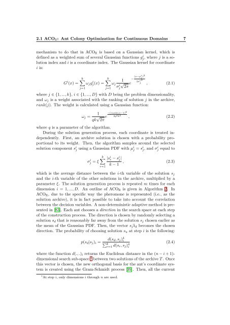
2.1 ACOR: Ant Colony Optimization for Continuous Domains 7
mechanism to do that in ACOR is based on a Gaussian kernel, which is
defined as a weighted sum of several Gaussian functions gi j , where j is a solution
index and i is a coordinate index. The Gaussian kernel for coordinate
i is:
G i k
(x) = ωjg
j=1
i k 1
j(x) = ωj
j=1 σi √ e
j 2π
− (x−µi j )2
2σi 2
j
, (2.1)
where j ∈ {1, ..., k}, i ∈ {1, ..., D} with D being the problem dimensionality,
and ωj is a weight associated with the ranking of solution j in the archive,
rank(j). The weight is calculated using a Gaussian function:
1
ωj =
qk √ 2π
e −(rank(j)−1)2
2q 2 k 2 , (2.2)
where q is a parameter of the algorithm.
During the solution generation process, each coordinate is treated independently.
First, an archive solution is chosen with a probability pro-
portional to its weight. Then, the algorithm samples around the selected
solution component si j using a Gaussian PDF with µij = sij , and σi j equal to
σ i k |s
j = ξ
r=1
i r − si j |
k − 1
, (2.3)
which is the average distance between the i-th variable of the solution sj
and the i-th variable of the other solutions in the archive, multiplied by a
parameter ξ. The solution generation process is repeated m times for each
dimension i = 1, ..., D. An outline of ACOR is given in Algorithm 2. In
ACOR, due to the specific way the pheromone is represented (i.e., as the
solution archive), it is in fact possible to take into account the correlation
between the decision variables. A non-deterministic adaptive method is presented
in [83]. Each ant chooses a direction in the search space at each step
of the construction process. The direction is chosen by randomly selecting a
solution sd that is reasonably far away from the solution sj chosen earlier as
the mean of the Gaussian PDF. Then, the vector sjsd becomes the chosen
direction. The probability of choosing solution su at step i is the following:
p(sd|sj)i =
d(sd, sj) 4 i
kr=1 d(sr, sj) 4 i
(2.4)
where the function d(., .)i returns the Euclidean distance in the (n − i + 1)dimensional
search sub-space 1 between two solutions of the archive T . Once
this vector is chosen, the new orthogonal basis for the ant’s coordinate system
is created using the Gram-Schmidt process [39]. Then, all the current
1 At step i, only dimensions i through n are used.