Improved ant colony optimization algorithms for continuous ... - CoDE

More documents

Recommendations

Info

10 Ant Colony Optimization of Sep-ACOR. In the following Chapter 3, an improved ACO algorithm is presented. ellipsoid, threshold= 1e−10 rotatedellipsoid, threshold= 1e−10 Numbers of Evaluations Numbers of Evaluations Numbers of Evaluations 50000 40000 30000 20000 10000 0 6000 5000 4000 3000 2000 1000 10000 8000 6000 4000 2000 0 q=1e−04 mant=2 k=50 xi=0.85 ACOrC−d2 ACOrC−d2 ACOrR−d2 ACOrC−d6 ACOrR−d6 ACOrC−d10 ACOrR−d10 ACOrC−d15 tablet, threshold= 1e−10 q=1e−04 mant=2 k=50 xi=0.85 ACOrC−d2 ACOrR−d2 ACOrC−d6 ACOrR−d6 ACOrC−d10 ACOrR−d10 ACOrC−d15 cigar, threshold= 1e−10 q=1e−04 mant=2 k=50 xi=0.85 ACOrR−d2 ACOrC−d6 ACOrR−d6 ACOrC−d10 ACOrR−d10 ACOrC−d15 ACOrR−d15 ACOrR−d15 ACOrR−d15 Numbers of Evaluations Numbers of Evaluations Numbers of Evaluations 60000 50000 40000 30000 20000 10000 0 6000 5000 4000 3000 2000 1000 10000 8000 6000 4000 2000 0 q=1e−04 mant=2 k=50 xi=0.85 ACOrC−d2 ACOrC−d2 ACOrR−d2 ACOrR−d2 ACOrC−d6 ACOrC−d6 ACOrR−d6 ACOrR−d6 ACOrC−d10 ACOrC−d10 ACOrR−d10 ACOrR−d10 ACOrC−d15 ACOrC−d15 ACOrR−d15 rotatedtablet, threshold= 1e−10 q=1e−04 mant=2 k=50 xi=0.85 ACOrC−d2 ACOrR−d2 ACOrC−d6 ACOrR−d6 ACOrC−d10 ACOrR−d10 ACOrC−d15 ACOrR−d15 rotatedcigar, threshold= 1e−10 q=1e−04 mant=2 k=50 xi=0.85 Figure 2.1: The box-plot comparison between C++ and R implementation of ACOR on different dimensionality. ACOrC is the C++ implementation of ACOR and ACOrR is the original R implementation. The left box plots are shown the numbers of function evaluations when achieving the threshold of solution quality in non-rotated functions, on the right box-plots those of rotated functions. We set the threshold of solution quality to 1e−10. The adopted parameter configurations of ACOR are shown in the legends. ACOrR−d15
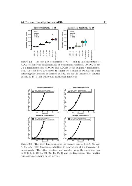
2.2 Further Investigation on ACOR Numbers of evaluations 5000 4000 3000 2000 1000 0 ackley, threshold= 1e−04 q=0.1 mant=2 k=50 xi=0.85 ACOrC−d2 ACOrR−d2 ACOrC−d4 ACOrR−d4 ACOrC−d6 ACOrR−d6 ACOrC−d10 ACOrR−d10(96%) Numbers of evaluations 10000 8000 6000 4000 2000 0 rosenbrock, threshold= 1e−04 q=0.1 mant=2 k=50 xi=0.85 Figure 2.2: The box-plot comparison of C++ and R implementation of ACOR on different dimensionality of benchmark functions. ACOrC is the C++ implementation of ACOR and ACOrR is the original R implementation. The box plots are shown the numbers of function evaluations when achieving the threshold of solution quality. We set the threshold of solution quality to 1e−04 for ackley and rosenbrock functions. Average of executive time (seconds) 0 20 40 60 80 100 Average of executive time (seconds) 0 20 40 60 80 100 ellipsoid−1000 evaluations ACOr (0.036)x^2+(−0.084)x+(0.97) Sep−ACOr (4e−08)x^2+(0.0019)x+(0.025) 0 20 40 60 80 100 dimensions rosenbrock−1000 evaluations ACOr (0.047)x^2+(−0.41)x+(2.4) Sep−ACOr (4.6e−06)x^2+(0.0014)x+(0.029) 0 20 40 60 80 100 dimensions Average of executive time (seconds) 0 20 40 60 80 100 Average of executive time (seconds) 0 20 40 60 80 100 ACOrC−d2 ACOrR−d2 ACOrC−d4 ACOrR−d4 ACOrC−d6 ACOrR−d6(88%) ACOrC−d10 sphere−1000 evaluations ACOr (0.028)x^2+(0.28)x+(−0.66) Sep−ACOr (−1.4e−05)x^2+(0.0022)x+(0.022) ACOrR−d10(92%) 0 20 40 60 80 100 dimensions rastrigin−1000 evaluations ACOr (0.033)x^2+(0.073)x+(0.25) Sep−ACOr (3.9e−06)x^2+(0.0015)x+(0.029) 0 20 40 60 80 100 dimensions Figure 2.3: The fitted functions show the average time of Sep-ACOR and ACOR after 1000 functions evaluations in dependence of the increasing dimensionality. The fitted functions are modeled using the execution time on 2, 3, 5, 7, 10, 15, 20, 25, 30, 35, 40 and 45 dimensions. The function expressions are shown in the legends. 11
Page 1: Université Libre de Bruxelles Facu
Page 5: Acknowledgements I thank Prof. Marc
Page 9 and 10: Contents Abstract iii Acknowledgeme
Page 11 and 12: Chapter 1 Introduction Metaheuristi
Page 13: them in the smallest function evalu
Page 16 and 17: 6 Ant Colony Optimization Algorithm
Page 18 and 19: 8 Ant Colony Optimization Algorithm
Page 22 and 23: 12 Ant Colony Optimization Average
Page 25 and 26: Chapter 3 An Incremental Ant Colony
Page 27 and 28: 3.2 IACOR with Local Search 17 3.2
Page 29 and 30: 3.3 Experimental Study 19 Algorithm
Page 31 and 32: 3.3 Experimental Study 21 Table 3.2
Page 33 and 34: 3.4 Conclusions 23 3.4 Conclusions
Page 35 and 36: 3.4 Conclusions 25 G−CMA−ES (5
Page 37: 3.4 Conclusions 27 Table 3.4: The m
Page 40 and 41: 30 Ant Colony Optimization for Mixe
Page 66 and 67: 56 Conclusions and Future Work of t
Page 69 and 70: Chapter 6 Appendix 6.1 Mathematical
Page 71 and 72:
6.1 Mathematical formulation of eng
Page 73 and 74:
6.1 Mathematical formulation of eng
Page 75 and 76:
Bibliography [1] K. Abhishek, S. Le
Page 77 and 78:
BIBLIOGRAPHY 67 [20] D. Datta and J
Page 79 and 80:
BIBLIOGRAPHY 69 [44] Q. He and L. W
Page 81 and 82:
BIBLIOGRAPHY 71 [65] S. Lucidi, V.
Page 83 and 84:
BIBLIOGRAPHY 73 [87] Thomas Stützl
show all

Improved ant colony optimization algorithms for continuous ... - CoDE

You also want an ePaper? Increase the reach of your titles

Delete template?

Save as template?