Improved ant colony optimization algorithms for continuous ... - CoDE

More documents

Recommendations

Info

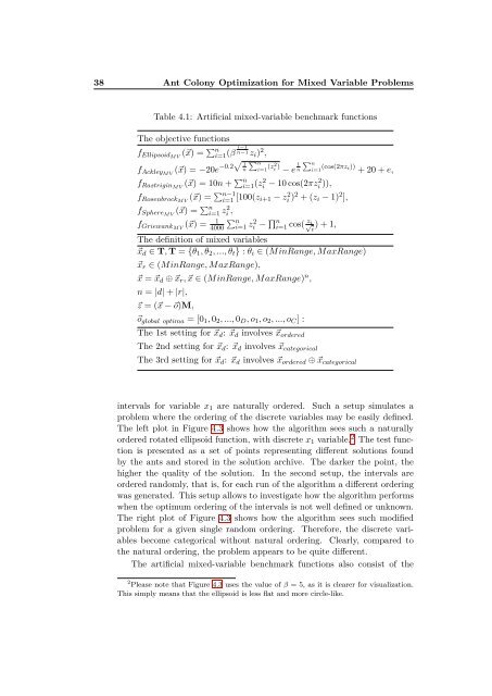
38 Ant Colony Optimization for Mixed Variable Problems Table 4.1: Artificial mixed-variable benchmark functions The objective functions fEllipsoidMV (x) = n i=1 (β i−1 n−1 zi) 2 , fAckleyMV (x) = −20e−0.2 1 n n i=1 (z2 i ) − e 1 n fRastriginMV (x) = 10n + n i=1 (z 2 i − 10 cos(2πz2 i )), n i=1 (cos(2πzi)) + 20 + e, fRosenbrockMV (x) = n−1 i=1 [100(zi+1 − z 2 i )2 + (zi − 1) 2 ], fSphereMV (x) = n i=1 z 2 i , fGriewankMV (x) = 1 4000 ni=1 z2 i − n i=1 cos( zi √ ) + 1, i The definition of mixed variables xd ∈ T, T = {θ1, θ2, ..., θt} : θi ∈ (MinRange, MaxRange) xr ∈ (MinRange, MaxRange), x = xd ⊕ xr, x ∈ (MinRange, MaxRange) n , n = |d| + |r|, z = (x − o)M, oglobal optima = [01, 02, ..., 0D, o1, o2, ..., oC] : The 1st setting for xd: xd involves xordered The 2nd setting for xd: xd involves xcategorical The 3rd setting for xd: xd involves xordered ⊕ xcategorical intervals for variable x1 are naturally ordered. Such a setup simulates a problem where the ordering of the discrete variables may be easily defined. The left plot in Figure 4.3 shows how the algorithm sees such a naturally ordered rotated ellipsoid function, with discrete x1 variable. 2 The test function is presented as a set of points representing different solutions found by the ants and stored in the solution archive. The darker the point, the higher the quality of the solution. In the second setup, the intervals are ordered randomly, that is, for each run of the algorithm a different ordering was generated. This setup allows to investigate how the algorithm performs when the optimum ordering of the intervals is not well defined or unknown. The right plot of Figure 4.3 shows how the algorithm sees such modified problem for a given single random ordering. Therefore, the discrete variables become categorical without natural ordering. Clearly, compared to the natural ordering, the problem appears to be quite different. The artificial mixed-variable benchmark functions also consist of the 2 Please note that Figure 4.3 uses the value of β = 5, as it is clearer for visualization. This simply means that the ellipsoid is less flat and more circle-like.
4.4 Performance Evaluation of ACOMV-o and ACOMV-c 39 X2 −2 0 2 4 6 Natural −2 0 2 4 6 X1 X2 −2 0 2 4 6 Random −2 0 2 4 6 Figure 4.3: Randomly rotated ellipsoid function (β = 5) with discrete variable x1 ∈ T, |T| = t = 30. The left plot presents the case in which the natural ordering of the intervals is used, while the right one presents the case in which a random ordering is used. characteristics such as non-separable, ill-conditioned and multi-modal. Nonseparate functions often exhibit intricate dependencies between decision variables. Ill-conditioned functions, like fRosenbrockMV , often lead to premature convergence. Multi-modal functions, like fAckleyMV , fRastriginMV and fGriewankMV , serves to find effectively a search globally in a highly multimodal topography [43]. For example, in the continuous study of [8], we can see PSO performs well on the separable problems. However, on nonseparable problems, PSO exhibits a strong performance decline, and PSO also performs very poorly even on moderately ill-conditioned functions, let alone in mixed-variable optimization cases. Therefore, the proposed artificial mixed-variable benchmark functions are expected to lead a challenge for different mixed-variable optimization algorithms. In anther aspect, the flexible discrete intervals and dimensions of the proposed benchmark functions are not only helpful for investigating the performance scalability of mixed-variable optimization algorithms, but also provide a convenient environment for automatic parameter tuning in mixed-variable optimization solvers generalization, thereby facing unseen real-world complex engineering optimization problems. 4.4 Performance Evaluation of ACOMV-o and ACOMV-c ACOMV-o and ACOMV-c represent a continuous relaxation approach and a native mixed-variable optimization approach on handling discrete variables, X1
Page 1: Université Libre de Bruxelles Facu
Page 5: Acknowledgements I thank Prof. Marc
Page 9 and 10: Contents Abstract iii Acknowledgeme
Page 11 and 12: Chapter 1 Introduction Metaheuristi
Page 13: them in the smallest function evalu
Page 16 and 17: 6 Ant Colony Optimization Algorithm
Page 18 and 19: 8 Ant Colony Optimization Algorithm
Page 20 and 21: 10 Ant Colony Optimization of Sep-A
Page 22 and 23: 12 Ant Colony Optimization Average
Page 25 and 26: Chapter 3 An Incremental Ant Colony
Page 27 and 28: 3.2 IACOR with Local Search 17 3.2
Page 29 and 30: 3.3 Experimental Study 19 Algorithm
Page 31 and 32: 3.3 Experimental Study 21 Table 3.2
Page 33 and 34: 3.4 Conclusions 23 3.4 Conclusions
Page 35 and 36: 3.4 Conclusions 25 G−CMA−ES (5
Page 37: 3.4 Conclusions 27 Table 3.4: The m
Page 40 and 41: 30 Ant Colony Optimization for Mixe
Page 66 and 67: 56 Conclusions and Future Work of t
Page 69 and 70: Chapter 6 Appendix 6.1 Mathematical
Page 71 and 72: 6.1 Mathematical formulation of eng
Page 73 and 74: 6.1 Mathematical formulation of eng
Page 75 and 76: Bibliography [1] K. Abhishek, S. Le
Page 77 and 78: BIBLIOGRAPHY 67 [20] D. Datta and J
Page 79 and 80: BIBLIOGRAPHY 69 [44] Q. He and L. W
Page 81 and 82: BIBLIOGRAPHY 71 [65] S. Lucidi, V.
Page 83 and 84: BIBLIOGRAPHY 73 [87] Thomas Stützl

Improved ant colony optimization algorithms for continuous ... - CoDE

You also want an ePaper? Increase the reach of your titles

Delete template?

Save as template?