Quantum GIS Training Manual - the QGIS Training Manual!
Quantum GIS Training Manual - the QGIS Training Manual!
Quantum GIS Training Manual - the QGIS Training Manual!

You also want an ePaper? Increase the reach of your titles
YUMPU automatically turns print PDFs into web optimized ePapers that Google loves.
<strong>Quantum</strong> <strong>GIS</strong> <strong>Training</strong> <strong>Manual</strong><br />
Release 1.0<br />
R. Thiede, T. Sutton, H. Düster, M. Sutton<br />
July 15, 2013
Contents<br />
1 Foreword 1<br />
1.1 Background . . . . . . . . . . . . . . . . . . . . . . . . . . . . . . . . . . . . 1<br />
1.2 License . . . . . . . . . . . . . . . . . . . . . . . . . . . . . . . . . . . . . . 1<br />
1.3 Sponsoring Chapters . . . . . . . . . . . . . . . . . . . . . . . . . . . . . . . 2<br />
1.4 Authors . . . . . . . . . . . . . . . . . . . . . . . . . . . . . . . . . . . . . . 3<br />
1.5 Individual Contributors . . . . . . . . . . . . . . . . . . . . . . . . . . . . . . 3<br />
1.6 Sponsors . . . . . . . . . . . . . . . . . . . . . . . . . . . . . . . . . . . . . 3<br />
1.7 Data . . . . . . . . . . . . . . . . . . . . . . . . . . . . . . . . . . . . . . . . 3<br />
1.8 Latest Version . . . . . . . . . . . . . . . . . . . . . . . . . . . . . . . . . . 3<br />
2 Module: The Interface 5<br />
2.1 Lesson: A Brief Introduction . . . . . . . . . . . . . . . . . . . . . . . . . . . 5<br />
2.2 Lesson: Adding your first layer . . . . . . . . . . . . . . . . . . . . . . . . . 7<br />
2.3 Lesson: An Overview of <strong>the</strong> Interface . . . . . . . . . . . . . . . . . . . . . . 8<br />
3 Module: Creating a Basic Map 13<br />
3.1 Lesson: Working with Vector Data . . . . . . . . . . . . . . . . . . . . . . . 13<br />
3.2 Lesson: Symbology . . . . . . . . . . . . . . . . . . . . . . . . . . . . . . . 16<br />
4 Module: Classifying Vector Data 49<br />
4.1 Lesson: Attribute Data . . . . . . . . . . . . . . . . . . . . . . . . . . . . . . 49<br />
4.2 Lesson: The Label Tool . . . . . . . . . . . . . . . . . . . . . . . . . . . . . 50<br />
4.3 Lesson: Classification . . . . . . . . . . . . . . . . . . . . . . . . . . . . . . 65<br />
5 Module: Creating Maps 89<br />
5.1 Lesson: Using Map Composer . . . . . . . . . . . . . . . . . . . . . . . . . . 89<br />
5.2 Assignment 1 . . . . . . . . . . . . . . . . . . . . . . . . . . . . . . . . . . . 104<br />
6 Module: Creating Vector Data 105<br />
6.1 Lesson: Creating a New Vector Dataset . . . . . . . . . . . . . . . . . . . . . 105<br />
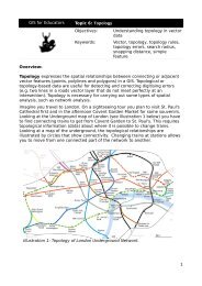
6.2 Lesson: Feature Topology . . . . . . . . . . . . . . . . . . . . . . . . . . . . 118<br />
6.3 Lesson: Forms . . . . . . . . . . . . . . . . . . . . . . . . . . . . . . . . . . 135<br />
6.4 Lesson: Actions . . . . . . . . . . . . . . . . . . . . . . . . . . . . . . . . . 148<br />
7 Module: Vector Analysis 159<br />
i
7.1 Lesson: Reprojecting and Transforming Data . . . . . . . . . . . . . . . . . . 159<br />
7.2 Lesson: Vector Analysis . . . . . . . . . . . . . . . . . . . . . . . . . . . . . 169<br />
7.3 Lesson: Network Analysis . . . . . . . . . . . . . . . . . . . . . . . . . . . . 187<br />
7.4 Lesson: Spatial Statistics . . . . . . . . . . . . . . . . . . . . . . . . . . . . . 201<br />
8 Module: Rasters 221<br />
8.1 Lesson: Working with Raster Data . . . . . . . . . . . . . . . . . . . . . . . . 221<br />
8.2 Lesson: Changing Raster Symbology . . . . . . . . . . . . . . . . . . . . . . 224<br />
8.3 Lesson: Terrain Analysis . . . . . . . . . . . . . . . . . . . . . . . . . . . . . 229<br />
9 Module: Completing <strong>the</strong> Analysis 239<br />
9.1 Lesson: Raster to Vector Conversion . . . . . . . . . . . . . . . . . . . . . . 239<br />
9.2 Lesson: Combining <strong>the</strong> Analyses . . . . . . . . . . . . . . . . . . . . . . . . 242<br />
9.3 Assignment . . . . . . . . . . . . . . . . . . . . . . . . . . . . . . . . . . . . 244<br />
9.4 Lesson: Supplementary Exercise . . . . . . . . . . . . . . . . . . . . . . . . 244<br />
10 Module: Plugins 261<br />
10.1 Lesson: Installing and Managing Plugins . . . . . . . . . . . . . . . . . . . . 261<br />
10.2 Lesson: Useful Q<strong>GIS</strong> Plugins . . . . . . . . . . . . . . . . . . . . . . . . . . 264<br />
11 Module: Online Resources 277<br />
11.1 Lesson: Web Mapping Services . . . . . . . . . . . . . . . . . . . . . . . . . 277<br />
11.2 Lesson: Web Feature Services . . . . . . . . . . . . . . . . . . . . . . . . . . 284<br />
12 Module: GRASS 293<br />
12.1 Lesson: GRASS Setup . . . . . . . . . . . . . . . . . . . . . . . . . . . . . . 293<br />
12.2 Lesson: GRASS Tools . . . . . . . . . . . . . . . . . . . . . . . . . . . . . . 305<br />
13 Module: Assessment 311<br />
13.1 Create a base map . . . . . . . . . . . . . . . . . . . . . . . . . . . . . . . . 311<br />
13.2 Analyze <strong>the</strong> data . . . . . . . . . . . . . . . . . . . . . . . . . . . . . . . . . 314<br />
13.3 Final Map . . . . . . . . . . . . . . . . . . . . . . . . . . . . . . . . . . . . . 314<br />
14 Module: PostgreSQL 315<br />
14.1 Lesson: Introduction to Databases . . . . . . . . . . . . . . . . . . . . . . . . 315<br />
14.2 Lesson: Implementing <strong>the</strong> Data Model . . . . . . . . . . . . . . . . . . . . . 323<br />
14.3 Lesson: Adding Data to <strong>the</strong> Model . . . . . . . . . . . . . . . . . . . . . . . 332<br />
14.4 Lesson: Queries . . . . . . . . . . . . . . . . . . . . . . . . . . . . . . . . . 335<br />
14.5 Lesson: Views . . . . . . . . . . . . . . . . . . . . . . . . . . . . . . . . . . 341<br />
14.6 Lesson: Rules . . . . . . . . . . . . . . . . . . . . . . . . . . . . . . . . . . 342<br />
15 Module: Post<strong>GIS</strong> 345<br />
15.1 Lesson: Post<strong>GIS</strong> Setup . . . . . . . . . . . . . . . . . . . . . . . . . . . . . . 345<br />
15.2 Lesson: Simple Feature Model . . . . . . . . . . . . . . . . . . . . . . . . . . 349<br />
15.3 Lesson: Import and Export . . . . . . . . . . . . . . . . . . . . . . . . . . . . 356<br />
15.4 Lesson: Spatial Queries . . . . . . . . . . . . . . . . . . . . . . . . . . . . . 358<br />
15.5 Lesson: Geometry Construction . . . . . . . . . . . . . . . . . . . . . . . . . 368<br />
16 Appendix: Contributing To This <strong>Manual</strong> 377<br />
16.1 Downloading Resources . . . . . . . . . . . . . . . . . . . . . . . . . . . . . 377<br />
ii
16.2 <strong>Manual</strong> Format . . . . . . . . . . . . . . . . . . . . . . . . . . . . . . . . . . 377<br />
16.3 Adding a Module . . . . . . . . . . . . . . . . . . . . . . . . . . . . . . . . . 377<br />
16.4 Adding a Lesson . . . . . . . . . . . . . . . . . . . . . . . . . . . . . . . . . 379<br />
16.5 Adding a Section . . . . . . . . . . . . . . . . . . . . . . . . . . . . . . . . . 379<br />
16.6 Add a Conclusion . . . . . . . . . . . . . . . . . . . . . . . . . . . . . . . . 381<br />
16.7 Add a Fur<strong>the</strong>r Reading Section . . . . . . . . . . . . . . . . . . . . . . . . . 381<br />
16.8 Add a What’s Next Section . . . . . . . . . . . . . . . . . . . . . . . . . . . 381<br />
16.9 Using Markup . . . . . . . . . . . . . . . . . . . . . . . . . . . . . . . . . . 381<br />
16.10 Thank You! . . . . . . . . . . . . . . . . . . . . . . . . . . . . . . . . . . . . 384<br />
17 Answer Sheet 385<br />
17.1 Results for Adding Your First Layer . . . . . . . . . . . . . . . . . . . . . . . 385<br />
17.2 Results for An Overview of <strong>the</strong> Interface . . . . . . . . . . . . . . . . . . . . . 385<br />
17.3 Results for Working with Vector Data . . . . . . . . . . . . . . . . . . . . . . 386<br />
17.4 Results for Symbology . . . . . . . . . . . . . . . . . . . . . . . . . . . . . . 387<br />
17.5 Results for Attribute Data . . . . . . . . . . . . . . . . . . . . . . . . . . . . 394<br />
17.6 Results for The Label Tool . . . . . . . . . . . . . . . . . . . . . . . . . . . . 395<br />
17.7 Results for Classification . . . . . . . . . . . . . . . . . . . . . . . . . . . . . 399<br />
17.8 Results for Creating a New Vector Dataset . . . . . . . . . . . . . . . . . . . 400<br />
17.9 Results for Vector Analysis . . . . . . . . . . . . . . . . . . . . . . . . . . . . 408<br />
17.10 Results for Raster Analysis . . . . . . . . . . . . . . . . . . . . . . . . . . . . 411<br />
17.11 Results for Completing <strong>the</strong> Analysis . . . . . . . . . . . . . . . . . . . . . . . 416<br />
17.12 Results for WMS . . . . . . . . . . . . . . . . . . . . . . . . . . . . . . . . . 424<br />
17.13 Results for Spatial Queries . . . . . . . . . . . . . . . . . . . . . . . . . . . . 428<br />
17.14 Results for Geometry Construction . . . . . . . . . . . . . . . . . . . . . . . 428<br />
17.15 Results for Simple Feature Model . . . . . . . . . . . . . . . . . . . . . . . . 429<br />
18 Indices and tables 431<br />
iii
1.1 Background<br />
CHAPTER 1<br />
Foreword<br />
In 2008 we launched <strong>the</strong> Gentle Introduction to <strong>GIS</strong> 1 , a completely free, open content resource<br />
for people who want to learn about <strong>GIS</strong> without being overloaded with jargon and new terminology.<br />
It was sponsored by <strong>the</strong> South African government and has been a phenomenal success,<br />
with people all over <strong>the</strong> world writing to us to tell us how <strong>the</strong>y are using <strong>the</strong> materials to run<br />
University <strong>Training</strong> Courses, teach <strong>the</strong>mselves <strong>GIS</strong> and so on. The Gentle Introduction is not a<br />
software tutorial, but ra<strong>the</strong>r aims to be a generic text (although we used Q<strong>GIS</strong> in all examples)<br />
for someone learning about <strong>GIS</strong>. There is also <strong>the</strong> Q<strong>GIS</strong> manual which provides a detailed<br />
functional overview of <strong>the</strong> Q<strong>GIS</strong> application. However, it is not structured as a tutorial, but<br />
ra<strong>the</strong>r as a reference guide. At Linfiniti Consulting CC. we frequently run training courses and<br />
have realised that a third resource is needed - one that leads <strong>the</strong> reader sequentially through<br />
learning <strong>the</strong> key aspects of Q<strong>GIS</strong> in a trainer-trainee format - which prompted us to produce<br />
this work.<br />
This training manual is intended to provide all <strong>the</strong> materials needed to run a 5 day course on<br />
Q<strong>GIS</strong>, PostgreSQL and Post<strong>GIS</strong>. The course is structured with content to suit novice, intermediate<br />
and advanced users alike and has many exercises complete with annotated answers<br />
throughout <strong>the</strong> text.<br />
1.2 License<br />
The Free <strong>Quantum</strong> <strong>GIS</strong> <strong>Training</strong> <strong>Manual</strong> by Linfiniti Consulting CC. is licensed under<br />
a Creative Commons Attribution-NonCommercial-ShareAlike 3.0 Unported License.<br />
Based on a work at https://github.com/qgis/Q<strong>GIS</strong>-<strong>Training</strong>-<strong>Manual</strong>. Permissions beyond<br />
<strong>the</strong> scope of this license may be available at https://github.com/qgis/Q<strong>GIS</strong>-<strong>Training</strong>-<br />
<strong>Manual</strong>/blob/master/index.rst.<br />
1 http://linfiniti.com/dla<br />
1
<strong>Quantum</strong> <strong>GIS</strong> <strong>Training</strong> <strong>Manual</strong>, Release 1.0<br />
We have published this Q<strong>GIS</strong> training manual under a liberal license that allows you to freely<br />
copy, modify and redistribute this work. A complete copy of <strong>the</strong> license is available at <strong>the</strong> end<br />
of this document. In simple terms, <strong>the</strong> usage guidelines are as follows:<br />
• You may not represent this work as your own work, or remove any authorship text or<br />
credits from this work.<br />
• You may not redistribute this work under more restrictive permissions than those under<br />
which it was provided to you.<br />
• If you add a substantitive portion to <strong>the</strong> work and contribute it back to <strong>the</strong> project (at<br />
least one complete module) you may add your name to <strong>the</strong> end of <strong>the</strong> authors list for this<br />
document (which will appear on <strong>the</strong> front page)<br />
• If you contribute minor changes and corrections you may add yourself to <strong>the</strong> contributors<br />
list below.<br />
• If you translate this document in its entirety, you may add your name to <strong>the</strong> authors list<br />
in <strong>the</strong> form “Translated by Joe Blogs”.<br />
• If you sponsor a module or lesson, you may request <strong>the</strong> author to include an acknowledgement<br />
in <strong>the</strong> beginning of each lesson contributed, e.g.:<br />
Note: This lesson was sponsored by MegaCorp.<br />
• If you are unsure about what you may do under this license, please contact us at office@linfiniti.com<br />
2 and we will advise you if what you intend doing is acceptable.<br />
• If you publish this work under a self publishing site such as http:://lulu.com we request<br />
that you donate <strong>the</strong> profits to <strong>the</strong> Q<strong>GIS</strong> project.<br />
• You may not commercialise this work, except with <strong>the</strong> expressed permission of <strong>the</strong> authors.<br />
To be clear, by commercialisation we mean that you may not sell for profit, create<br />
commercial derivative works (e.g. selling content for use as articles in a magazine). The<br />
exception to this is if all <strong>the</strong> profits are given to <strong>the</strong> Q<strong>GIS</strong> project. You may (and we<br />
encourage you to do so) use this work as a text book when conducting training courses,<br />
even if <strong>the</strong> course itself is commercial in nature. In o<strong>the</strong>r words, you are welcome to<br />
make money by running a training course that uses this work as a text book, but you may<br />
not profit off <strong>the</strong> sales of <strong>the</strong> book itself - all such profits should be contributed back to<br />
Q<strong>GIS</strong>.<br />
1.3 Sponsoring Chapters<br />
This work is by no means a complete treatise on all <strong>the</strong> things you can do with Q<strong>GIS</strong> and we<br />
encourage o<strong>the</strong>rs to add new materials to fill any gaps. Linfiniti Consulting CC. can also create<br />
additional materials for you as a commercial service, with <strong>the</strong> understanding that all such works<br />
produced should become part of <strong>the</strong> core content and be published under <strong>the</strong> same license.<br />
2 office@linfiniti.com<br />
2 Chapter 1. Foreword
1.4 Authors<br />
<strong>Quantum</strong> <strong>GIS</strong> <strong>Training</strong> <strong>Manual</strong>, Release 1.0<br />
• Rüdiger Thiede (rudi@linfiniti.com 3 ) - Rudi has written <strong>the</strong> Q<strong>GIS</strong> instructional materials<br />
and parts of <strong>the</strong> Post<strong>GIS</strong> materials.<br />
• Tim Sutton (tim@linfiniti.com 4 ) - Tim has overseen and guided <strong>the</strong> project and coauthored<br />
<strong>the</strong> PostgreSQL and Post<strong>GIS</strong> parts. Tim also authored <strong>the</strong> custom sphinx <strong>the</strong>me<br />
used for this manual.<br />
• Horst Düster (horst.duester@kappasys.ch 5 ) - Horst co-authored <strong>the</strong> PostgreSQL and<br />
Post<strong>GIS</strong> parts<br />
• Marcelle Sutton (marcelle@linfiniti.com 6 ) - Marcelle provided proof reading and editorial<br />
advice during <strong>the</strong> creation of this work.<br />
1.5 Individual Contributors<br />
Your name here!<br />
1.6 Sponsors<br />
• Cape Peninsula University of Technology<br />
1.7 Data<br />
The sample data that accompanies this resource is freely available and comes from <strong>the</strong> following<br />
sources:<br />
• Streets and Places datasets from OpenStreetMap (http://www.openstreetmap.org/)<br />
• Property boundaries (urban and rural), water bodies from NGI (http://www.ngi.gov.za/)<br />
• SRTM DEM from <strong>the</strong> CGIAR-CGI (http://srtm.csi.cgiar.org/)<br />
1.8 Latest Version<br />
You can always obtain <strong>the</strong> latest version of this document by visiting our home page 7 which is<br />
kindly hosted by http://read<strong>the</strong>docs.org.<br />
3 rudi@linfiniti.com<br />
4 tim@linfiniti.com<br />
5 horst.duester@kappasys.ch<br />
6 marcelle@linfiniti.com<br />
7 http://read<strong>the</strong>docs.org/builds/<strong>the</strong>-free-qgis-training-manual/<br />
1.4. Authors 3
<strong>Quantum</strong> <strong>GIS</strong> <strong>Training</strong> <strong>Manual</strong>, Release 1.0<br />
Note: There are links to PDF and epub versions of <strong>the</strong> documentation in <strong>the</strong> lower right hand<br />
corner of <strong>the</strong> above mentioned home page.<br />
Tim Sutton, May 2012<br />
4 Chapter 1. Foreword
2.1 Lesson: A Brief Introduction<br />
CHAPTER 2<br />
Module: The Interface<br />
Welcome to our course! Over <strong>the</strong> next few days, we’ll be showing you how to use Q<strong>GIS</strong> easily<br />
and efficiently. If you’re new to <strong>GIS</strong>, we’ll tell you what you need to get started. If you’re an<br />
experienced user, you’ll see how Q<strong>GIS</strong> fulfills all <strong>the</strong> functions you expect from a <strong>GIS</strong> program,<br />
and more!<br />
In this module we introduce <strong>the</strong> Q<strong>GIS</strong> project itself, as well as explaining <strong>the</strong> user interface.<br />
After completing this section, you will be able to correctly identify <strong>the</strong> main elements of <strong>the</strong><br />
screen in Q<strong>GIS</strong> and know what each of <strong>the</strong>m does, and load a shapefile into Q<strong>GIS</strong>.<br />
Warning: This course includes instructions on adding, deleting and altering <strong>GIS</strong> datasets.<br />
We have provided training datasets for this purpose. Before using <strong>the</strong> techniques described<br />
here on your own data, always ensure you have proper backups!<br />
2.1.1 How to use this tutorial<br />
Any text that looks like this refers to something on <strong>the</strong> screen that you can click on.<br />
Text that looks → like → this directs you through menus.<br />
This kind of text refers to something you can type, such as a command, path, or file<br />
name.<br />
2.1.2 Tiered course objectives<br />
This course caters to different user experience levels. Depending on which category you consider<br />
yourself to be in, you can expect a different set of course outcomes. Each category<br />
contains information that is essential for <strong>the</strong> next one, so it’s important to do all exercises that<br />
are at or below your level of experience.<br />
5
<strong>Quantum</strong> <strong>GIS</strong> <strong>Training</strong> <strong>Manual</strong>, Release 1.0<br />
Basic<br />
In this category, <strong>the</strong> course assumes that you have little or no prior experience with <strong>the</strong>oretical<br />
<strong>GIS</strong> knowledge or <strong>the</strong> operation of a <strong>GIS</strong> program.<br />
Limited <strong>the</strong>oretical background will be provided to explain <strong>the</strong> purpose of an action you will<br />
be performing in <strong>the</strong> program, but <strong>the</strong> emphasis is on learning by doing.<br />
When you complete <strong>the</strong> course, you will have a better concept of <strong>the</strong> possibilities of <strong>GIS</strong>, and<br />
how to harness <strong>the</strong>ir power via Q<strong>GIS</strong>.<br />
Intermediate<br />
In this category, it is assumed that you have working knowledge and experience of <strong>the</strong> everyday<br />
uses of <strong>GIS</strong>.<br />
Following <strong>the</strong> instructions for <strong>the</strong> beginner level will provide you with familiar ground, as well<br />
as to make you aware of <strong>the</strong> cases where Q<strong>GIS</strong> does things slightly differently from o<strong>the</strong>r<br />
software you may be used to. You will also learn how to use analysis functions in Q<strong>GIS</strong>.<br />
When you complete <strong>the</strong> course, you should be comfortable with using Q<strong>GIS</strong> for all of <strong>the</strong><br />
functions you usually need from a <strong>GIS</strong> for everyday use.<br />
Advanced<br />
In this category, <strong>the</strong> assumption is that you are experienced with <strong>GIS</strong>, have knowledge of and<br />
experience with spatial databases, using data on a remote server, perhaps writing scripts for<br />
analysis purposes, etc.<br />
Following <strong>the</strong> instructions for <strong>the</strong> o<strong>the</strong>r two levels will familiarize you with <strong>the</strong> approach that<br />
<strong>the</strong> Q<strong>GIS</strong> interface follows, and will ensure that you know how to access <strong>the</strong> basic functions<br />
that you need. You will also be shown how to make use of Q<strong>GIS</strong>’ plugin system, database<br />
access system, and so on.<br />
When you complete <strong>the</strong> course, you should be well-acquainted with <strong>the</strong> everyday operation of<br />
Q<strong>GIS</strong>, as well as its more advanced functions.<br />
2.1.3 Why Q<strong>GIS</strong>?<br />
As information becomes increasingly spatially aware, <strong>the</strong>re is no shortage of tools able to fulfill<br />
some or all commonly used <strong>GIS</strong> functions. Why should anyone be using Q<strong>GIS</strong> over some o<strong>the</strong>r<br />
<strong>GIS</strong> software package?<br />
Here are only some of <strong>the</strong> reasons:<br />
• It’s free, as in lunch. Installing and using <strong>the</strong> Q<strong>GIS</strong> program costs you a grand total of<br />
zero money. No initial fee, no recurring fee, nothing.<br />
6 Chapter 2. Module: The Interface
<strong>Quantum</strong> <strong>GIS</strong> <strong>Training</strong> <strong>Manual</strong>, Release 1.0<br />
• It’s free, as in liberty. If you need extra functionality in Q<strong>GIS</strong>, you can do more than<br />
just hope it will be included in <strong>the</strong> next release. You can sponsor <strong>the</strong> development of a<br />
feature, or add it yourself if you are familiar with programming.<br />
• It’s constantly developing. Because anyone can add new features and improve on existing<br />
ones, Q<strong>GIS</strong> never stagnates. The development of a new tool can happen as quickly as<br />
you need it to.<br />
• Extensive help and documentation is available. If you’re stuck with anything, you can<br />
turn to <strong>the</strong> extensive documentation, your fellow Q<strong>GIS</strong> users, or even <strong>the</strong> developers.<br />
• Cross-platform. Q<strong>GIS</strong> can be installed on MacOS, Windows and Linux.<br />
Now that you know why you want to use Q<strong>GIS</strong>, we can show you how. The first lesson will<br />
guide you in creating your first Q<strong>GIS</strong> map.<br />
2.2 Lesson: Adding your first layer<br />
We will start <strong>the</strong> application, and create a basic map to use for examples and exercises.<br />
The goal for this lesson: To get started with an example map.<br />
Note: Before starting this exercise, Q<strong>GIS</strong> must be installed on your computer.<br />
Launch Q<strong>GIS</strong> from its desktop shortcut, menu item, etc., depending on how you configured its<br />
installation.<br />
Note: The screenshots for this course were taken in Q<strong>GIS</strong> 1.8 running on Ubuntu 11.10 and<br />
Windows XP. Depending on your setup, <strong>the</strong> screens you encounter may well appear somewhat<br />
different. However, all <strong>the</strong> same buttons will still be available, and <strong>the</strong> instructions will work<br />
on any OS. You will need Q<strong>GIS</strong> 1.8 (<strong>the</strong> latest version at time of writing) to use this course.<br />
Let’s get started right away!<br />
2.2.1 Follow along: Prepare a map<br />
• Open Q<strong>GIS</strong>. You will have a new, blank map.<br />
• Look for <strong>the</strong> Add Vector Layer button:<br />
• Click on it to open <strong>the</strong> following dialog:<br />
2.2. Lesson: Adding your first layer 7
<strong>Quantum</strong> <strong>GIS</strong> <strong>Training</strong> <strong>Manual</strong>, Release 1.0<br />
• Click on <strong>the</strong> Browse button and navigate to <strong>the</strong> file exercise_data/streets.shp<br />
(in your course directory). With this file selected, click Open. You will see <strong>the</strong> original<br />
dialog, but with <strong>the</strong> file path filled in. Click Open here as well. The data you specified<br />
will now load.<br />
Congratulations! You now have a basic map. Now would be a good time to save your work.<br />
• Click on <strong>the</strong> Save As button:<br />
• Save <strong>the</strong> map under exercise_data/ and call it basic_map.qgs.<br />
Check your results<br />
2.2.2 In conclusion<br />
You’ve learned how to add a layer and create a basic map!<br />
2.2.3 What’s next?<br />
Now you’re familiar with <strong>the</strong> function of <strong>the</strong> Add Vector Layer button, but what about all <strong>the</strong><br />
o<strong>the</strong>rs? How does this interface work? Before we go on with <strong>the</strong> more involved stuff, let’s first<br />
take a good look at <strong>the</strong> general layout of <strong>the</strong> Q<strong>GIS</strong> interface. This is <strong>the</strong> topic of <strong>the</strong> next lesson.<br />
2.3 Lesson: An Overview of <strong>the</strong> Interface<br />
We will explore <strong>the</strong> Q<strong>GIS</strong> user interface so that you are familiar with <strong>the</strong> menus, toolbars, map<br />
canvas and layers list that form <strong>the</strong> basic structure of <strong>the</strong> interface.<br />
8 Chapter 2. Module: The Interface
<strong>Quantum</strong> <strong>GIS</strong> <strong>Training</strong> <strong>Manual</strong>, Release 1.0<br />
The goal for this lesson: To understand <strong>the</strong> basics of <strong>the</strong> Q<strong>GIS</strong> user interface.<br />
2.3.1 Try yourself...: The Basics<br />
The elements identified in <strong>the</strong> figure above are:<br />
1. Layers list<br />
2. Toolbars<br />
3. Map canvas<br />
4. Status bar<br />
The Layers List<br />
In <strong>the</strong> Layers list, you can see a list, at any time, of all <strong>the</strong> layers available to you.<br />
Expanding collapsed items (by clicking <strong>the</strong> arrow or plus symbol beside <strong>the</strong>m) will provide<br />
you with more information on <strong>the</strong> layer’s current appearance.<br />
2.3. Lesson: An Overview of <strong>the</strong> Interface 9
<strong>Quantum</strong> <strong>GIS</strong> <strong>Training</strong> <strong>Manual</strong>, Release 1.0<br />
Right-clicking on a layer will give you a menu with lots of extra options. You will be using<br />
some of <strong>the</strong>m before long, so take a look around!<br />
Some versions of Q<strong>GIS</strong> have a separate Control rendering order checkbox just underneath <strong>the</strong><br />
Layers list. Don’t worry if you can’t see it. If it is present, ensure that it’s checked for now.<br />
Note: A vector layer is a dataset, usually of a specific kind of object, such as roads, trees, etc.<br />
A vector layer can consist of ei<strong>the</strong>r points, lines or polygons.<br />
Toolbars<br />
Your most oft-used sets of tools can be turned into toolbars for basic access. For example, <strong>the</strong><br />
File toolbar allows you to save, load, print, and start a new project. You can easily customize<br />
<strong>the</strong> interface to see only <strong>the</strong> tools you use most often, adding or removing toolbars as necessary<br />
via <strong>the</strong> View → Toolbars menu.<br />
Even if <strong>the</strong>y are not visible in a toolbar, all of your tools will remain accessible via <strong>the</strong> menus.<br />
For example, if you remove <strong>the</strong> File toolbar (which contains <strong>the</strong> Save button), you can still save<br />
your map by clicking on <strong>the</strong> File menu and <strong>the</strong>n clicking on Save.<br />
The Map Canvas<br />
This is where <strong>the</strong> map itself is displayed.<br />
The Status Bar<br />
Shows you information about <strong>the</strong> current map. Also allows you to adjust <strong>the</strong> map scale and see<br />
<strong>the</strong> mouse cursor’s coordinates on <strong>the</strong> map.<br />
2.3.2 Try yourself... 1<br />
Try to identify <strong>the</strong> four elements listed above on your own screen, without referring to <strong>the</strong><br />
diagram above. See if you can identify <strong>the</strong>ir names and functions. You will become more<br />
familiar with <strong>the</strong>se elements as you use <strong>the</strong>m in <strong>the</strong> coming days.<br />
Check your results<br />
2.3.3 Try yourself... 2<br />
Try to find each of <strong>the</strong>se tools on your screen. What is <strong>the</strong>ir purpose?<br />
10 Chapter 2. Module: The Interface
1.<br />
2.<br />
3.<br />
4.<br />
5.<br />
<strong>Quantum</strong> <strong>GIS</strong> <strong>Training</strong> <strong>Manual</strong>, Release 1.0<br />
Hint: If any of <strong>the</strong>se tools is not visible on <strong>the</strong> screen, try enabling some toolbars that are<br />
currently hidden. Also keep in mind that if <strong>the</strong>re isn’t enough space on <strong>the</strong> screen, a toolbar<br />
may be shortened by hiding some of its tools. You can see <strong>the</strong> hidden tools by clicking on <strong>the</strong><br />
double right arrow button in any such collapsed toolbar. You can see a tooltip with <strong>the</strong> name of<br />
any tool by holding your mouse over <strong>the</strong> tool for a while.<br />
Check your results<br />
2.3.4 What’s next?<br />
Now you’ve seen how <strong>the</strong> Q<strong>GIS</strong> interface works, you can use <strong>the</strong> tools available to you and<br />
start improving on your map! This is <strong>the</strong> topic of <strong>the</strong> next lesson.<br />
2.3. Lesson: An Overview of <strong>the</strong> Interface 11
<strong>Quantum</strong> <strong>GIS</strong> <strong>Training</strong> <strong>Manual</strong>, Release 1.0<br />
12 Chapter 2. Module: The Interface
CHAPTER 3<br />
Module: Creating a Basic Map<br />
In this module, you will create a basic map which will be used later as a basis for fur<strong>the</strong>r<br />
demonstrations of Q<strong>GIS</strong>’ functionality.<br />
3.1 Lesson: Working with Vector Data<br />
Vector data is arguably <strong>the</strong> most common kind of data you will find in <strong>the</strong> daily use of <strong>GIS</strong>. It<br />
describes geographic data in terms of points, that may be connected into lines and polygons.<br />
Every object in a vector dataset is called a feature, and is associated with data that describes<br />
that feature.<br />
The goal for this lesson: To learn about <strong>the</strong> structure of vector data, and how to load vector<br />
datasets into a map.<br />
3.1.1 Follow along: Viewing layer attributes<br />
It’s important to know that <strong>the</strong> data you will be working with does not only represent where<br />
objects are in space, but also tells you what those objects are.<br />
From <strong>the</strong> previous exercise, you should have <strong>the</strong> streets layer loaded in your map. What you<br />
can see right now is merely <strong>the</strong> position of <strong>the</strong> roads.<br />
To see all <strong>the</strong> data available to you:<br />
• Click on this button:<br />
It will show you a table with more data about <strong>the</strong> streets layer. This extra data is called attribute<br />
data. The lines that you can see on your map represent where <strong>the</strong> streets go; this is <strong>the</strong> spatial<br />
data.<br />
These definitions are commonly used in <strong>GIS</strong>, so it’s essential to remember <strong>the</strong>m!<br />
• You may now close <strong>the</strong> attribute table.<br />
13
<strong>Quantum</strong> <strong>GIS</strong> <strong>Training</strong> <strong>Manual</strong>, Release 1.0<br />
Vector data represents features in terms of points, lines and polygons on a coordinate plane. It<br />
is usually used to store discrete features, like roads and city blocks.<br />
3.1.2 Follow along: Loading vector data from shapefiles<br />
The Shapefile is a specific file format that allows you to store <strong>GIS</strong> data in an associated group of<br />
files. Each layer consists of several files with <strong>the</strong> same name, but different file types. Shapefiles<br />
are easy to send back and forth, and most <strong>GIS</strong> software can read <strong>the</strong>m.<br />
Refer back to <strong>the</strong> introductory exercise in <strong>the</strong> previous section for instructions on how to add<br />
vector layers.<br />
• Load <strong>the</strong> “places” dataset into your map following <strong>the</strong> same method.<br />
Check your results<br />
3.1.3 Follow along: Loading vector data from a database<br />
Databases allow you to store a large volume of associated data in one file. You may already<br />
be familiar with a database management system (DBMS) such as Microsoft Access. <strong>GIS</strong> applications<br />
can also make use of databases. <strong>GIS</strong>-specific DBMSes (such as Post<strong>GIS</strong>) have extra<br />
functions, because <strong>the</strong>y need to handle spatial data.<br />
• Click on this icon:<br />
(If you’re sure you can’t see it at all, check that <strong>the</strong> Manage Layers toolbar is enabled.)<br />
It will give you a new dialog. In this dialog:<br />
• Click <strong>the</strong> New button.<br />
• In <strong>the</strong> same folder as <strong>the</strong> o<strong>the</strong>r data, you should find <strong>the</strong> file land_use.db. Select it and<br />
click Open.<br />
You will now see <strong>the</strong> first dialog again. Notice that <strong>the</strong> dropdown select above <strong>the</strong> three buttons<br />
now reads “land_use.db@...”, followed by <strong>the</strong> path of <strong>the</strong> database file on your computer.<br />
• Click <strong>the</strong> Connect button. You should see this in <strong>the</strong> previously empty box:<br />
• Click on <strong>the</strong> first layer to select it, <strong>the</strong>n use shift+click to select all of <strong>the</strong>m at once.<br />
• Click Add. This will add all three layers to <strong>the</strong> map at once.<br />
14 Chapter 3. Module: Creating a Basic Map
<strong>Quantum</strong> <strong>GIS</strong> <strong>Training</strong> <strong>Manual</strong>, Release 1.0<br />
Note: Remember to save <strong>the</strong> map often! The map file doesn’t contain any of <strong>the</strong> data directly,<br />
but it remembers which layers you loaded into your map.<br />
Check your results<br />
3.1.4 Follow along: Reordering <strong>the</strong> layers<br />
The layers in your Layers list are drawn on <strong>the</strong> map in a certain order. The layer at <strong>the</strong> bottom<br />
of <strong>the</strong> list is drawn first, and <strong>the</strong> layer at <strong>the</strong> top is drawn last. By changing <strong>the</strong> order that <strong>the</strong>y<br />
are shown on <strong>the</strong> list, you can change <strong>the</strong> order <strong>the</strong>y are drawn in.<br />
Note: Depending on <strong>the</strong> version of Q<strong>GIS</strong> that you are using, you may have a checkbox beneath<br />
your Layers list reading Control rendering order. This must be checked (switched on) so that<br />
moving <strong>the</strong> layers up and down in <strong>the</strong> Layers list will bring <strong>the</strong>m to <strong>the</strong> front or send <strong>the</strong>m to<br />
<strong>the</strong> back in <strong>the</strong> map. If your version of Q<strong>GIS</strong> doesn’t have this option, <strong>the</strong>n it is switched on by<br />
default and you don’t need to worry about it.<br />
The order in which <strong>the</strong> layers have been loaded into <strong>the</strong> map is probably not logical at this<br />
stage. It’s possible that <strong>the</strong> road layer is completely hidden because o<strong>the</strong>r layers are on top of<br />
it.<br />
For example, this layer order...<br />
... would result in roads and places being hidden as <strong>the</strong>y run underneath urban areas.<br />
To resolve this problem:<br />
• Click and drag on a layer in <strong>the</strong> Layers list.<br />
• Reorder <strong>the</strong>m to look like this:<br />
3.1. Lesson: Working with Vector Data 15
<strong>Quantum</strong> <strong>GIS</strong> <strong>Training</strong> <strong>Manual</strong>, Release 1.0<br />
3.1.5 In conclusion<br />
Now you’ve added all <strong>the</strong> layers you need from several different sources.<br />
3.1.6 What’s next?<br />
Using <strong>the</strong> random palette automatically assigned when loading <strong>the</strong> layers, your current map<br />
is probably not easy to read. It would be preferable to assign your own choice of colors and<br />
symbols. This is what you’ll learn to do in <strong>the</strong> next lesson.<br />
3.2 Lesson: Symbology<br />
The symbology of a layer is its visual appearance on <strong>the</strong> map. The basic strength of <strong>GIS</strong> over<br />
o<strong>the</strong>r ways of representing data with spatial aspects is that with <strong>GIS</strong>, you have a dynamic visual<br />
representation of <strong>the</strong> data you’re working with.<br />
Therefore, <strong>the</strong> visual appearance of <strong>the</strong> map (which depends on <strong>the</strong> symbology of <strong>the</strong> individual<br />
layers) is very important. The end user of <strong>the</strong> maps you produce will need to be able to easily<br />
see what <strong>the</strong> map represents. Equally as important, you need to be able to explore <strong>the</strong> data as<br />
you’re working with it, and good symbology helps a lot.<br />
In o<strong>the</strong>r words, having proper symbology is not a luxury or just nice to have. In fact, it’s<br />
essential for you to use a <strong>GIS</strong> properly and produce maps and information that people will be<br />
able to use.<br />
The goal for this lesson: To be able to create any symbology you want for any vector layer.<br />
16 Chapter 3. Module: Creating a Basic Map
3.2.1 Follow along: Changing colors<br />
<strong>Quantum</strong> <strong>GIS</strong> <strong>Training</strong> <strong>Manual</strong>, Release 1.0<br />
To change a layer’s symbology, open its Layer Properties. Let’s begin by changing <strong>the</strong> color<br />
of <strong>the</strong> urban layer.<br />
• Right-click on <strong>the</strong> urban layer in <strong>the</strong> Layers list.<br />
• Select <strong>the</strong> menu item Properties in <strong>the</strong> menu that appears.<br />
Note: By default, you can also access a layer’s properties by double-clicking on <strong>the</strong> layer in<br />
<strong>the</strong> Layers list.<br />
In <strong>the</strong> Properties window:<br />
• Select <strong>the</strong> Style tab at <strong>the</strong> extreme left:<br />
• Click <strong>the</strong> Change button next to <strong>the</strong> Color label.<br />
3.2. Lesson: Symbology 17
<strong>Quantum</strong> <strong>GIS</strong> <strong>Training</strong> <strong>Manual</strong>, Release 1.0<br />
A standard color dialog will appear.<br />
• Choose a grey color and click OK.<br />
• Click OK again in <strong>the</strong> Layer Properties window, and you will see <strong>the</strong> color change being<br />
applied to <strong>the</strong> layer.<br />
3.2.2 Try yourself...<br />
Change <strong>the</strong> rural layer to a new color that you associate with rural farming areas.<br />
Check your results<br />
3.2.3 Follow along: Changing symbol structure<br />
This is good stuff so far, but <strong>the</strong>re’s more to a layer’s symbology than just its color. Next we<br />
want to change <strong>the</strong> color of <strong>the</strong> farms (<strong>the</strong> rural layer), but we also want to eliminate <strong>the</strong> lines<br />
between <strong>the</strong> different farms so as to make <strong>the</strong> map less visually cluttered.<br />
• Open <strong>the</strong> Layer Properties window for <strong>the</strong> rural layer.<br />
18 Chapter 3. Module: Creating a Basic Map
<strong>Quantum</strong> <strong>GIS</strong> <strong>Training</strong> <strong>Manual</strong>, Release 1.0<br />
Under <strong>the</strong> Style tab, you will see <strong>the</strong> same kind of dialog as before. This time, however, you’re<br />
doing more than just quickly changing <strong>the</strong> color.<br />
• Click on <strong>the</strong> Change... button below <strong>the</strong> color display:<br />
The Symbol properties dialog will appear.<br />
• Change <strong>the</strong> color inside <strong>the</strong> polygons in <strong>the</strong> layer by clicking <strong>the</strong> button next to <strong>the</strong> Color<br />
label (if you haven’t done so already during <strong>the</strong> previous lesson).<br />
• In <strong>the</strong> dialog that appears, choose a new color (that seems to suit a farm).<br />
• Click OK, but only once.<br />
Next, we want to get rid of <strong>the</strong> lines between all <strong>the</strong> farms.<br />
• Click on <strong>the</strong> Border style dropdown. At <strong>the</strong> moment, it should be showing a short line<br />
and <strong>the</strong> words Solid Line.<br />
• Change this to No Pen.<br />
3.2. Lesson: Symbology 19
<strong>Quantum</strong> <strong>GIS</strong> <strong>Training</strong> <strong>Manual</strong>, Release 1.0<br />
• Click OK, and <strong>the</strong>n OK again.<br />
Now <strong>the</strong> rural layer won’t have any lines between farms.<br />
3.2.4 Try yourself...<br />
• Change <strong>the</strong> urban layer’s symbology so that it is gray and without outlines.<br />
• Change <strong>the</strong> rural layer again so that it has dotted outlines which are just a bit darker than<br />
<strong>the</strong> fill color for that layer.<br />
Check your results<br />
3.2.5 Follow along: Scale-based visibility<br />
Sometimes you will find that a layer is not suitable for a given scale. For example, a dataset<br />
of all <strong>the</strong> continents may have low detail, and not be very accurate at street level. When that<br />
happens, you want to be able to hide <strong>the</strong> dataset at inappropriate scales.<br />
In our case, we may decide to hide <strong>the</strong> streets from view at small scales. This map, for example<br />
...<br />
... is not very useful. The streets are just a blob at that scale.<br />
To enable scale-based rendering:<br />
• Open <strong>the</strong> Layer Properties dialog for <strong>the</strong> streets layer.<br />
• Activate <strong>the</strong> General tab.<br />
20 Chapter 3. Module: Creating a Basic Map
<strong>Quantum</strong> <strong>GIS</strong> <strong>Training</strong> <strong>Manual</strong>, Release 1.0<br />
• Enable scale-based rendering by clicking on <strong>the</strong> checkbox labeled Use scale dependent<br />
rendering:<br />
• Change <strong>the</strong> Maximum value to 100000.<br />
• Click OK.<br />
Test <strong>the</strong> effects of this by zooming in and out in your map, noting when <strong>the</strong> streets layer disappears<br />
and reappears.<br />
Note: You can use your mouse wheel to zoom in increments. Alternatively, use <strong>the</strong> zoom tools<br />
to zoom to a window:<br />
3.2. Lesson: Symbology 21
<strong>Quantum</strong> <strong>GIS</strong> <strong>Training</strong> <strong>Manual</strong>, Release 1.0<br />
3.2.6 Follow along: Adding symbol layers<br />
Now that you know how to change simple symbology for layers, <strong>the</strong> next step is to create more<br />
complex symbology. Q<strong>GIS</strong> allows you to do this using symbol layers.<br />
• Go back to <strong>the</strong> rural layer’s Symbol properties dialog as before.<br />
In this example, <strong>the</strong> current symbol has no outline (i.e., it uses <strong>the</strong> No Pen border style).<br />
Note <strong>the</strong> highlighted button.<br />
• Click on it and <strong>the</strong> dialog will change to look somewhat like this:<br />
22 Chapter 3. Module: Creating a Basic Map
<strong>Quantum</strong> <strong>GIS</strong> <strong>Training</strong> <strong>Manual</strong>, Release 1.0<br />
(It may appear somewhat different in color, for example, but you’re going to change that anyway.)<br />
Now <strong>the</strong>re’s a second symbol layer. Being a solid color, it will of course completely hide <strong>the</strong><br />
previous kind of symbol. Plus, it has a Solid Line border style, which we don’t want. Clearly<br />
this symbol has to be changed.<br />
Note: It’s important not to get confused between a map layer and a symbol layer. A map layer<br />
is a vector (or raster) that has been loaded into <strong>the</strong> map. A symbol layer is part of <strong>the</strong> symbol<br />
used to represent a map layer. This course will usually refer to a map layer as just a layer, but<br />
a symbol layer will always be called a symbol layer, to prevent confusion.<br />
• Set <strong>the</strong> border style to No Pen, as before.<br />
• Change <strong>the</strong> fill style to something o<strong>the</strong>r than Solid or No brush. For example:<br />
3.2. Lesson: Symbology 23
<strong>Quantum</strong> <strong>GIS</strong> <strong>Training</strong> <strong>Manual</strong>, Release 1.0<br />
• Click OK in this dialog and Apply in <strong>the</strong> one after that. Now you can see your results and<br />
tweak <strong>the</strong>m as needed.<br />
You can even add multiple extra symbol layers and create a kind of texture for your layer that<br />
way.<br />
24 Chapter 3. Module: Creating a Basic Map
It’s fun! But it probably has too many colors to use in a real map...<br />
3.2.7 Try yourself...<br />
<strong>Quantum</strong> <strong>GIS</strong> <strong>Training</strong> <strong>Manual</strong>, Release 1.0<br />
• Create a simple, but not distracting texture for <strong>the</strong> rural layer using <strong>the</strong> methods above.<br />
Check your results<br />
3.2.8 Follow along: Enabling symbol levels<br />
When symbol layers are rendered, <strong>the</strong>y are also rendered in a sequence, similar to how <strong>the</strong><br />
different map layers are rendered. This means that in some cases, having many symbol layers<br />
in one symbol can cause unexpected results.<br />
• Give <strong>the</strong> streets layer an extra symbol layer (using <strong>the</strong> methid for adding symbol layers<br />
demonstrated above).<br />
• Give <strong>the</strong> base line a thickness of 2.0.<br />
• Give <strong>the</strong> top layer a thickness of 0.5.<br />
You’ll notice that this happens:<br />
3.2. Lesson: Symbology 25
<strong>Quantum</strong> <strong>GIS</strong> <strong>Training</strong> <strong>Manual</strong>, Release 1.0<br />
Well that’s not what we want at all!<br />
To prevent this from happening, you can enable symbol levels, which will control <strong>the</strong> order in<br />
which <strong>the</strong> different symbol layers are rendered.<br />
• In <strong>the</strong> Layer Properties dialog, click on Advanced → Symbol levels:<br />
26 Chapter 3. Module: Creating a Basic Map
The Symbol Levels dialog will appear.<br />
• Alter its values to match this example:<br />
<strong>Quantum</strong> <strong>GIS</strong> <strong>Training</strong> <strong>Manual</strong>, Release 1.0<br />
3.2. Lesson: Symbology 27
<strong>Quantum</strong> <strong>GIS</strong> <strong>Training</strong> <strong>Manual</strong>, Release 1.0<br />
• Click OK, <strong>the</strong>n OK again.<br />
The map will now look like this:<br />
28 Chapter 3. Module: Creating a Basic Map
<strong>Quantum</strong> <strong>GIS</strong> <strong>Training</strong> <strong>Manual</strong>, Release 1.0<br />
When you’re done, remember to save <strong>the</strong> symbol itself so as not to lose your work if you<br />
change <strong>the</strong> symbol again in <strong>the</strong> future. You can save your current symbol style by clicking <strong>the</strong><br />
Save Style ... button under <strong>the</strong> Style tab of <strong>the</strong> Layer Properties dialog. Save your style under<br />
exercise_data/styles. You can load a previously saved style at any time by clicking<br />
<strong>the</strong> Load Style ... button. Before you change a style, keep in mind that any unsaved style you<br />
are replacing will be lost.<br />
3.2.9 Try yourself...<br />
• Change <strong>the</strong> appearance of <strong>the</strong> streets layer again.<br />
The roads must be dark gray or black, with a thin yellow outline, and a dashed white line<br />
running in <strong>the</strong> middle to make <strong>the</strong>m resemble a real road.<br />
Check your results<br />
3.2.10 Try yourself...<br />
Symbol levels also work for classified layers (i.e., layers having multiple symbols). Since we<br />
haven’t covered classification yet, you will work with some rudimentary preclassified data.<br />
3.2. Lesson: Symbology 29
<strong>Quantum</strong> <strong>GIS</strong> <strong>Training</strong> <strong>Manual</strong>, Release 1.0<br />
• Create a new map and add only <strong>the</strong> streets dataset.<br />
• Apply <strong>the</strong> style advanced_levels_demo.qml provided in<br />
exercise_data/styles.<br />
• Zoom to <strong>the</strong> Swellendam area (<strong>the</strong> cluster of roads near <strong>the</strong> center of <strong>the</strong> layer).<br />
• Using symbol layers, ensure that <strong>the</strong> outlines of layers flow into one ano<strong>the</strong>r as per <strong>the</strong><br />
image below:<br />
Check your results<br />
3.2.11 Follow along: Symbol layer types<br />
In addition to setting fill colors and using predefined patterns, you can use different symbol<br />
layer types entirely. The only type we’ve been using up to now was <strong>the</strong> Simple Fill type. The<br />
more advanced symbol layer types allow you to customize your symbols even fur<strong>the</strong>r.<br />
Each type of vector (point, line and polygon) has its own set of symbol layer types. First we<br />
will look at <strong>the</strong> types available for points.<br />
Point symbol layer types<br />
• Change <strong>the</strong> symbol properties for <strong>the</strong> places layer:<br />
30 Chapter 3. Module: Creating a Basic Map
• You can access <strong>the</strong> various symbol layer types here:<br />
<strong>Quantum</strong> <strong>GIS</strong> <strong>Training</strong> <strong>Manual</strong>, Release 1.0<br />
3.2. Lesson: Symbology 31
<strong>Quantum</strong> <strong>GIS</strong> <strong>Training</strong> <strong>Manual</strong>, Release 1.0<br />
• Investigate <strong>the</strong> various options available to you, and choose a symbol layer type o<strong>the</strong>r<br />
than <strong>the</strong> default Simple Marker.<br />
• If in doubt, use an Ellipse Marker.<br />
• Choose a white outline and black fill, with a symbol width of 2,00 and symbol height of<br />
4,00.<br />
Line symbol layer types<br />
To see <strong>the</strong> various options available for line data:<br />
• Change <strong>the</strong> symbol layer type for <strong>the</strong> street layer’s topmost symbol layer:<br />
• Click on <strong>the</strong> Change button next to <strong>the</strong> Marker label.<br />
• Change <strong>the</strong> symbol properties to match this dialog:<br />
32 Chapter 3. Module: Creating a Basic Map
• Change <strong>the</strong> interval to 2,00:<br />
<strong>Quantum</strong> <strong>GIS</strong> <strong>Training</strong> <strong>Manual</strong>, Release 1.0<br />
• Ensure that <strong>the</strong> symbol levels are correct before applying <strong>the</strong> style.<br />
3.2. Lesson: Symbology 33
<strong>Quantum</strong> <strong>GIS</strong> <strong>Training</strong> <strong>Manual</strong>, Release 1.0<br />
Once you have applied <strong>the</strong> style, take a look at its results on <strong>the</strong> map. As you can see, <strong>the</strong>se<br />
symbols change direction along with <strong>the</strong> road but don’t always bend along with it. This is<br />
useful for some purposes, but not for o<strong>the</strong>rs. If you prefer, you can change <strong>the</strong> symbol layer in<br />
question back to <strong>the</strong> way it was before.<br />
Polygon symbol layer types<br />
To see <strong>the</strong> various options available for polygon data:<br />
• Change <strong>the</strong> symbol layer type for <strong>the</strong> urban layer, as before for <strong>the</strong> o<strong>the</strong>r layers.<br />
• Investigate what <strong>the</strong> different options on <strong>the</strong> list can do.<br />
• Choose one of <strong>the</strong>m that you find suitable.<br />
• If in doubt, use <strong>the</strong> Point pattern fill with <strong>the</strong> following options:<br />
34 Chapter 3. Module: Creating a Basic Map
• Add a new symbol layer with a normal Simple fill.<br />
• Make it gray with no outlines.<br />
<strong>Quantum</strong> <strong>GIS</strong> <strong>Training</strong> <strong>Manual</strong>, Release 1.0<br />
• Move it underneath <strong>the</strong> point pattern symbol layer with <strong>the</strong> Move down button:<br />
3.2. Lesson: Symbology 35
<strong>Quantum</strong> <strong>GIS</strong> <strong>Training</strong> <strong>Manual</strong>, Release 1.0<br />
As a result, you have a textured symbol for <strong>the</strong> urban layer, with <strong>the</strong> added benefit that you can<br />
change <strong>the</strong> size, shape and distance of <strong>the</strong> individual dots that make up <strong>the</strong> texture.<br />
3.2.12 Follow along: Creating a custom SVG fill<br />
Note: To do this exercise, you will need to have <strong>the</strong> free vector editing software Inkscape<br />
installed.<br />
• Start <strong>the</strong> Inkscape program.<br />
You will see <strong>the</strong> following interface:<br />
36 Chapter 3. Module: Creating a Basic Map
<strong>Quantum</strong> <strong>GIS</strong> <strong>Training</strong> <strong>Manual</strong>, Release 1.0<br />
You should find this familiar if you have used o<strong>the</strong>r vector image editing programs, like Corel.<br />
• Change <strong>the</strong> canvas to a size appropriate for a small texture.<br />
• Click on <strong>the</strong> menu item File → Document Properties. This will give you <strong>the</strong> Document<br />
Properties dialog.<br />
• Change <strong>the</strong> Units to px.<br />
3.2. Lesson: Symbology 37
<strong>Quantum</strong> <strong>GIS</strong> <strong>Training</strong> <strong>Manual</strong>, Release 1.0<br />
• Change <strong>the</strong> Width and Height to 100.<br />
• Close <strong>the</strong> dialog when you are done.<br />
• Click on <strong>the</strong> menu item View → Zoom → Page to see <strong>the</strong> page you are working with.<br />
• Select <strong>the</strong> Circle tool:<br />
• Click and drag on <strong>the</strong> page to draw an ellipse. To make <strong>the</strong> ellipse turn into a circle, hold<br />
<strong>the</strong> ctrl button while you’re drawing it.<br />
• Right-click on <strong>the</strong> circle you just created and open its Fill and Stroke:<br />
38 Chapter 3. Module: Creating a Basic Map
• Change <strong>the</strong> Stroke paint to green:<br />
<strong>Quantum</strong> <strong>GIS</strong> <strong>Training</strong> <strong>Manual</strong>, Release 1.0<br />
3.2. Lesson: Symbology 39
<strong>Quantum</strong> <strong>GIS</strong> <strong>Training</strong> <strong>Manual</strong>, Release 1.0<br />
• Change <strong>the</strong> Stroke style to a thicker line:<br />
40 Chapter 3. Module: Creating a Basic Map
• Draw a line using <strong>the</strong> Line tool:<br />
<strong>Quantum</strong> <strong>GIS</strong> <strong>Training</strong> <strong>Manual</strong>, Release 1.0<br />
3.2. Lesson: Symbology 41
<strong>Quantum</strong> <strong>GIS</strong> <strong>Training</strong> <strong>Manual</strong>, Release 1.0<br />
• Click once to start <strong>the</strong> line. Hold ctrl to make it snap to increments of 15 degrees.<br />
• Click once to end <strong>the</strong> line segment, <strong>the</strong>n right-click to finalize <strong>the</strong> line.<br />
• Change its color and width as before and move it around as necessary, so that you end up<br />
with a symbol like this one:<br />
42 Chapter 3. Module: Creating a Basic Map
<strong>Quantum</strong> <strong>GIS</strong> <strong>Training</strong> <strong>Manual</strong>, Release 1.0<br />
• Save it under <strong>the</strong> directory that <strong>the</strong> course is in, under exercise_data/symbols, as<br />
an SVG file.<br />
In Q<strong>GIS</strong>:<br />
• Open <strong>the</strong> Layer Properties for <strong>the</strong> rural layer.<br />
• Change <strong>the</strong> symbol structure to <strong>the</strong> following:<br />
3.2. Lesson: Symbology 43
<strong>Quantum</strong> <strong>GIS</strong> <strong>Training</strong> <strong>Manual</strong>, Release 1.0<br />
• Find your SVG image via <strong>the</strong> Browse button:<br />
44 Chapter 3. Module: Creating a Basic Map
• Change <strong>the</strong> settings as shown:<br />
<strong>Quantum</strong> <strong>GIS</strong> <strong>Training</strong> <strong>Manual</strong>, Release 1.0<br />
3.2. Lesson: Symbology 45
<strong>Quantum</strong> <strong>GIS</strong> <strong>Training</strong> <strong>Manual</strong>, Release 1.0<br />
Your rural layer should now have a texture like <strong>the</strong> one on this map:<br />
46 Chapter 3. Module: Creating a Basic Map
3.2.13 In conclusion<br />
<strong>Quantum</strong> <strong>GIS</strong> <strong>Training</strong> <strong>Manual</strong>, Release 1.0<br />
Changing <strong>the</strong> symbology for <strong>the</strong> different layers has transformed a collection of vector files<br />
into a legible map. Not only can you see what’s happening, it’s even nice to look at!<br />
3.2.14 Fur<strong>the</strong>r reading<br />
Examples of Beautiful Maps 1<br />
3.2.15 What’s next?<br />
Changing symbols for whole layers is useful, but <strong>the</strong> information contained within each layer<br />
is not yet available to someone reading <strong>the</strong>se maps. What are <strong>the</strong> streets called? Which administrative<br />
regions do certain areas belong to? What are <strong>the</strong> relative surface areas of <strong>the</strong> farms?<br />
All of this information is still hidden. The next lesson will explain how to represent this data<br />
on your map.<br />
Note: Did you remember to save your map recently?<br />
1 http://gis.stackexchange.com/questions/3083/examples-of-beautiful-maps<br />
3.2. Lesson: Symbology 47
<strong>Quantum</strong> <strong>GIS</strong> <strong>Training</strong> <strong>Manual</strong>, Release 1.0<br />
48 Chapter 3. Module: Creating a Basic Map
CHAPTER 4<br />
Module: Classifying Vector Data<br />
Classifying vector data allows you to assign different symbols to features (different objects in<br />
<strong>the</strong> same layer), depending on <strong>the</strong>ir attributes. This allows someone who uses <strong>the</strong> map to easily<br />
see <strong>the</strong> attributes of various features.<br />
4.1 Lesson: Attribute Data<br />
Up to now, none of <strong>the</strong> changes we have made to <strong>the</strong> map have been influenced by <strong>the</strong> objects<br />
that are being shown. In o<strong>the</strong>r words, all <strong>the</strong> farms look alike, and all <strong>the</strong> roads look alike.<br />
When looking at <strong>the</strong> map, <strong>the</strong> viewers don’t know anything about <strong>the</strong> roads <strong>the</strong>y are seeing;<br />
only that <strong>the</strong>re is a road of a certain shape in a certain area.<br />
But <strong>the</strong> whole strength of <strong>GIS</strong> is that all <strong>the</strong> objects that are visible on <strong>the</strong> map, also have<br />
attributes. Maps in a <strong>GIS</strong> aren’t just pictures. They represent not only objects in locations, but<br />
also information about those objects.<br />
The goal of this lesson: To explore <strong>the</strong> attribute data of an object and understand what <strong>the</strong><br />
various data can be useful for.<br />
4.1.1 Follow along: Attribute data<br />
Open <strong>the</strong> attribute table for <strong>the</strong> places layer (refer back to <strong>the</strong> section “Working with Vector<br />
Data” if necessary). Which field would be <strong>the</strong> most useful to represent in label form, and why?<br />
Check your results<br />
4.1.2 In conclusion<br />
You now know how to use <strong>the</strong> attribute table to see what is actually in <strong>the</strong> data you’re using.<br />
Any dataset will only be useful to you if it has <strong>the</strong> attributes that you care about. If you know<br />
which attributes you need, you can quickly decide if you’re able to use a given dataset, or if<br />
you need to look for ano<strong>the</strong>r one that has <strong>the</strong> required attribute data.<br />
49
<strong>Quantum</strong> <strong>GIS</strong> <strong>Training</strong> <strong>Manual</strong>, Release 1.0<br />
4.1.3 What’s next?<br />
Different attributes are useful for different purposes. Some of <strong>the</strong>m can be represented directly<br />
as text for <strong>the</strong> map user to see. You’ll learn how to do this in <strong>the</strong> next lesson.<br />
4.2 Lesson: The Label Tool<br />
Labels can be added to a map to show any information about an object. Any vector layer can<br />
have labels associated with it. These labels rely on <strong>the</strong> attribute data of a layer for <strong>the</strong>ir content.<br />
Note: The Layer Properties dialog does have a Labels tab, but for this example we will not be<br />
using it. It has too few options and may be difficult to work with, which is why it will probably<br />
be taken out of new versions of Q<strong>GIS</strong> (after 1.8). Instead, for this lesson we’ll use <strong>the</strong> separate<br />
Label tool, which has more options and is more user-friendly.<br />
The goal for this lesson: To apply useful and good-looking labels to a layer.<br />
4.2.1 Follow along: Using labels<br />
Before being able to access <strong>the</strong> Label tool, you will need to ensure that it has been activated.<br />
• Go to <strong>the</strong> menu item View → Toolbars.<br />
• Ensure that <strong>the</strong> Label item has a check mark next to it. If it doesn’t, click on <strong>the</strong> Label<br />
item, and it will be activated.<br />
• Click on <strong>the</strong> places layer in <strong>the</strong> Layers list, so that it is highlighted.<br />
• Click on <strong>the</strong> following toolbar button:<br />
This gives you <strong>the</strong> Layer labeling settings dialog.<br />
• Check <strong>the</strong> box next to Label this layer with....<br />
50 Chapter 4. Module: Classifying Vector Data
<strong>Quantum</strong> <strong>GIS</strong> <strong>Training</strong> <strong>Manual</strong>, Release 1.0<br />
You’ll need to choose which field in <strong>the</strong> attributes will be used for <strong>the</strong> labels. In <strong>the</strong> previous<br />
lesson, you decided that <strong>the</strong> NAME field was <strong>the</strong> most suitable one for this purpose.<br />
• Select NAME from <strong>the</strong> list:<br />
4.2. Lesson: The Label Tool 51
<strong>Quantum</strong> <strong>GIS</strong> <strong>Training</strong> <strong>Manual</strong>, Release 1.0<br />
• Click OK.<br />
The map should now have labels like this:<br />
52 Chapter 4. Module: Classifying Vector Data
4.2.2 Follow along: Changing label options<br />
<strong>Quantum</strong> <strong>GIS</strong> <strong>Training</strong> <strong>Manual</strong>, Release 1.0<br />
What we have so far is good, but as you can see, <strong>the</strong> labels are overlapping <strong>the</strong> points that <strong>the</strong>y<br />
are associated with. That doesn’t look very nice. The text is also a bit larger than it needs to<br />
be. Let’s fix <strong>the</strong>se problems!<br />
• Open <strong>the</strong> Label tool again by clicking on its button as before.<br />
• Click on <strong>the</strong> ellipsis (...) button to change <strong>the</strong> text properties:<br />
4.2. Lesson: The Label Tool 53
<strong>Quantum</strong> <strong>GIS</strong> <strong>Training</strong> <strong>Manual</strong>, Release 1.0<br />
A standard text change dialog appears, similar to those in many o<strong>the</strong>r programs. Change <strong>the</strong><br />
font to Arial size 9. Your labels will now look like this:<br />
That’s <strong>the</strong> font problem solved! Now let’s look at <strong>the</strong> problem of <strong>the</strong> labels overlapping <strong>the</strong><br />
points, but before we do that, let’s take a look at <strong>the</strong> Buffer option.<br />
54 Chapter 4. Module: Classifying Vector Data
• Open <strong>the</strong> Label tool dialog.<br />
<strong>Quantum</strong> <strong>GIS</strong> <strong>Training</strong> <strong>Manual</strong>, Release 1.0<br />
• Deactivate <strong>the</strong> label buffer by clicking on <strong>the</strong> checkbox next to <strong>the</strong> text that says Buffer.<br />
• Click Apply.<br />
Note <strong>the</strong> effects in <strong>the</strong> map:<br />
Now you can see why we usually need label buffers!<br />
• Reactivate <strong>the</strong> buffers by clicking in <strong>the</strong> same checkbox as before, and <strong>the</strong>n clicking<br />
Apply.<br />
Back to <strong>the</strong> problem of <strong>the</strong> labels that overlap points.<br />
• In <strong>the</strong> Label tool dialog, go to <strong>the</strong> Advanced tab.<br />
• Change <strong>the</strong> value of Label distance to 2.<br />
4.2. Lesson: The Label Tool 55
<strong>Quantum</strong> <strong>GIS</strong> <strong>Training</strong> <strong>Manual</strong>, Release 1.0<br />
• Click Apply.<br />
This is <strong>the</strong> result:<br />
56 Chapter 4. Module: Classifying Vector Data
<strong>Quantum</strong> <strong>GIS</strong> <strong>Training</strong> <strong>Manual</strong>, Release 1.0<br />
4.2.3 Follow along: Using labels instead of layer symbology<br />
In many cases, <strong>the</strong> location of a point doesn’t need to be very specific. For example, most of<br />
<strong>the</strong> points in <strong>the</strong> places layer refer to entire towns or suburbs, and <strong>the</strong> specific point associated<br />
with such features is not that specific on a large scale. In fact, giving a point that is too specific<br />
is often confusing for someone reading a map.<br />
To name an example: on a map of <strong>the</strong> world, <strong>the</strong> point given for <strong>the</strong> European Union may<br />
be somewhere in Poland, for instance. To someone reading <strong>the</strong> map, seeing a point labeled<br />
European Union in Poland, it may seem that <strong>the</strong> capital of <strong>the</strong> European Union is <strong>the</strong>refore in<br />
Poland.<br />
So, to prevent this kind of misunderstanding, it’s often useful to deactivate <strong>the</strong> point symbols<br />
and replace <strong>the</strong>m completely with labels.<br />
In Q<strong>GIS</strong>, you can do this by changing <strong>the</strong> position of <strong>the</strong> labels to be rendered directly over <strong>the</strong><br />
points <strong>the</strong>y refer to.<br />
• Open <strong>the</strong> Layer labeling settings dialog for <strong>the</strong> places layer.<br />
• Go to <strong>the</strong> Advanced tab.<br />
• Click on <strong>the</strong> over point button.<br />
• Hide <strong>the</strong> point symbols by editing <strong>the</strong> layer style as usual, and setting <strong>the</strong> size of points<br />
4.2. Lesson: The Label Tool 57
<strong>Quantum</strong> <strong>GIS</strong> <strong>Training</strong> <strong>Manual</strong>, Release 1.0<br />
to 0:<br />
• Click OK and you’ll see this result:<br />
58 Chapter 4. Module: Classifying Vector Data
<strong>Quantum</strong> <strong>GIS</strong> <strong>Training</strong> <strong>Manual</strong>, Release 1.0<br />
As you can see, some of <strong>the</strong> labels are now missing to prevent overlap (at this scale). Sometimes<br />
this is what you want when dealing with datasets that have many points, but at o<strong>the</strong>r times you<br />
will lose useful information this way. There is ano<strong>the</strong>r possibility for handling cases like this,<br />
which we’ll cover in a later exercise in this lesson.<br />
4.2.4 Try yourself... Customize <strong>the</strong> labels<br />
• Return <strong>the</strong> label and symbol settings to <strong>the</strong> way <strong>the</strong>y were before.<br />
Check your results<br />
• Set <strong>the</strong> map to <strong>the</strong> scale 1:50000. You can do this by typing it into <strong>the</strong> Scale box in <strong>the</strong><br />
Status Bar.<br />
• Modify your labels to be suitable for viewing at this scale.<br />
Check your results<br />
4.2.5 Follow along: Labeling lines<br />
Now that you know how labeling works, <strong>the</strong>re’s an additional problem. Points and polygons<br />
are easy to label, but what about lines? If you label <strong>the</strong>m <strong>the</strong> same way as <strong>the</strong> points, your<br />
results would look like this:<br />
4.2. Lesson: The Label Tool 59
<strong>Quantum</strong> <strong>GIS</strong> <strong>Training</strong> <strong>Manual</strong>, Release 1.0<br />
This is not very useful! To make lines behave, we’ll need to edit some options.<br />
• Hide <strong>the</strong> places layer so that it doesn’t distract you.<br />
• Activate labels for <strong>the</strong> streets layer as before. (Remember to use <strong>the</strong> Label tool on <strong>the</strong><br />
toolbar, not <strong>the</strong> one in Label Properties!)<br />
• Set <strong>the</strong> font Size to 9 so that you can see more labels.<br />
• Zoom in on <strong>the</strong> Swellendam town area.<br />
• In <strong>the</strong> Label tool dialog’s Advanced tab, choose <strong>the</strong> following settings:<br />
60 Chapter 4. Module: Classifying Vector Data
The map will look somewhat like this, depending on scale:<br />
<strong>Quantum</strong> <strong>GIS</strong> <strong>Training</strong> <strong>Manual</strong>, Release 1.0<br />
4.2. Lesson: The Label Tool 61
<strong>Quantum</strong> <strong>GIS</strong> <strong>Training</strong> <strong>Manual</strong>, Release 1.0<br />
It’s better than before, but still not ideal. For starters, some of <strong>the</strong> names appear more than<br />
once, and that’s not always necessary. To prevent that from happening:<br />
• Enable <strong>the</strong> option Merge connected lines to avoid duplicate labels (also under <strong>the</strong> Advanced<br />
tab - you may need to scroll down to see it).<br />
Ano<strong>the</strong>r useful function is to prevent labels being drawn for features too short to be of notice.<br />
• Set <strong>the</strong> value of Suppress labeling of features smaller than ... to 5mm and note <strong>the</strong> results<br />
when you click Apply.<br />
Try out different Placement settings as well (also under <strong>the</strong> Advanced tab). As we’ve seen<br />
before, <strong>the</strong> horizontal option is not a good idea in this case, so let’s try <strong>the</strong> curved option<br />
instead!<br />
• Select <strong>the</strong> curved option under <strong>the</strong> Advanced tab of <strong>the</strong> Layer labeling settings dialog.<br />
Here’s <strong>the</strong> result:<br />
As you can see, this hides a lot of <strong>the</strong> labels that were previously visible, because of <strong>the</strong> difficulty<br />
of making some of <strong>the</strong>m follow twisting street lines and still be legible. You can decide<br />
which of <strong>the</strong>se options to use, depending on what you think seems more useful or what looks<br />
better.<br />
4.2.6 Follow along: Data defined settings<br />
• Deactivate labeling for <strong>the</strong> streets layer.<br />
62 Chapter 4. Module: Classifying Vector Data
• Reactivate labeling for <strong>the</strong> places layer.<br />
• Open <strong>the</strong> attribute table for places.<br />
<strong>Quantum</strong> <strong>GIS</strong> <strong>Training</strong> <strong>Manual</strong>, Release 1.0<br />
It has two fields that are of interest to us now: ADDR_CITY and IN_SWD. ADDR_CITY is <strong>the</strong><br />
city that <strong>the</strong> feature is in. IN_SWD is derived from it, and tells you whe<strong>the</strong>r or not that feature<br />
is in Swellendam (1 if it is, 0 if not). We can use this data to influence <strong>the</strong> label styles.<br />
• Navigate to <strong>the</strong> Data defined settings tab.<br />
• In <strong>the</strong> Italic dropdown, select IN_SWD and click Apply.<br />
Notice its effects:<br />
4.2.7 Try yourself... Using data defined settings<br />
Note: We’re jumping ahead a bit here to demonstrate some advanced labeling settings. At <strong>the</strong><br />
advanced level, it’s assumed that you’ll know what <strong>the</strong> following means. If you don’t, feel free<br />
to leave out this section and come back later when you’ve covered <strong>the</strong> requisite materials.<br />
• Open <strong>the</strong> attribute table for places.<br />
• Enter edit mode by clicking this button (at <strong>the</strong> lower edge of <strong>the</strong> attribute table):<br />
• Add a new column:<br />
• Configure it like this:<br />
4.2. Lesson: The Label Tool 63
<strong>Quantum</strong> <strong>GIS</strong> <strong>Training</strong> <strong>Manual</strong>, Release 1.0<br />
• Use this to set custom font sizes for each different type of place (i.e., each key in <strong>the</strong><br />
PLACE field).<br />
Check your results<br />
4.2.8 Fur<strong>the</strong>r possibilities with labeling<br />
We can’t cover every option in this course, but be aware that <strong>the</strong> Label tool has many o<strong>the</strong>r<br />
useful functions. You can set scale-based rendering, alter <strong>the</strong> rendering priority for labels in<br />
a layer, and set every label option using layer attributes. You can even set <strong>the</strong> rotation, XY<br />
position, and o<strong>the</strong>r properties of a label (if you have attribute fields allocated for <strong>the</strong> purpose),<br />
<strong>the</strong>n edit <strong>the</strong>se properties using <strong>the</strong> tools adjacent to <strong>the</strong> main Label tool:<br />
(These tools will be active if <strong>the</strong> required attribute fields exist and you are in edit mode.)<br />
Feel free to explore more possibilities of <strong>the</strong> labeling system.<br />
4.2.9 In conclusion<br />
You’ve learned how to use layer attributes to create dynamic labels. This can make your map a<br />
lot more informative and stylish!<br />
64 Chapter 4. Module: Classifying Vector Data
4.2.10 What’s next?<br />
<strong>Quantum</strong> <strong>GIS</strong> <strong>Training</strong> <strong>Manual</strong>, Release 1.0<br />
Now that you know how attributes can make a visual difference for your map, how about using<br />
<strong>the</strong>m to change <strong>the</strong> symbology of objects <strong>the</strong>mselves? That’s <strong>the</strong> topic for <strong>the</strong> next lesson!<br />
4.3 Lesson: Classification<br />
Labels are a good way to communicate information such as <strong>the</strong> names of individual places, but<br />
<strong>the</strong>y can’t be used for everything. For example, let’s say that someone wants to know which<br />
area <strong>the</strong> farms are in. Using labels, you’d get this:<br />
Obviously this is not ideal, so we need ano<strong>the</strong>r solution. That’s what this lesson is about!<br />
The goal for this lesson: To learn how to classify vector data effectively.<br />
4.3.1 Follow along: Classifying nominal data<br />
• Open Layer Properties.<br />
• Go to <strong>the</strong> Style tab.<br />
• Click on <strong>the</strong> dropdown that says Single Symbol:<br />
4.3. Lesson: Classification 65
<strong>Quantum</strong> <strong>GIS</strong> <strong>Training</strong> <strong>Manual</strong>, Release 1.0<br />
• Change it to Categorized and <strong>the</strong> interface will change:<br />
66 Chapter 4. Module: Classifying Vector Data
• Change <strong>the</strong> Column to TOWN and <strong>the</strong> Color ramp to random:<br />
<strong>Quantum</strong> <strong>GIS</strong> <strong>Training</strong> <strong>Manual</strong>, Release 1.0<br />
4.3. Lesson: Classification 67
<strong>Quantum</strong> <strong>GIS</strong> <strong>Training</strong> <strong>Manual</strong>, Release 1.0<br />
• Click <strong>the</strong> button labeled Classify and <strong>the</strong>n click OK.<br />
You’ll see something like this:<br />
68 Chapter 4. Module: Classifying Vector Data
<strong>Quantum</strong> <strong>GIS</strong> <strong>Training</strong> <strong>Manual</strong>, Release 1.0<br />
• Click <strong>the</strong> arrow (or plus sign) next to rural in <strong>the</strong> Layer list, you’ll see <strong>the</strong> categories<br />
explained:<br />
So, this is useful! But it hurts your eyes to look at it, so let’s see what we can do about that.<br />
• Open Layer Properties and go to <strong>the</strong> Style tab again.<br />
• Change <strong>the</strong> symbol:<br />
4.3. Lesson: Classification 69
<strong>Quantum</strong> <strong>GIS</strong> <strong>Training</strong> <strong>Manual</strong>, Release 1.0<br />
• Get rid of <strong>the</strong> outline <strong>the</strong> same way you did before, and click OK. (If you need to, go<br />
back to <strong>the</strong> lesson where we covered this to remember how it’s done.)<br />
• Click <strong>the</strong> Delete all button:<br />
70 Chapter 4. Module: Classifying Vector Data
This gets rid of <strong>the</strong> ugly classes so you can try again.<br />
• Click Classify again, and <strong>the</strong> new symbols will appear.<br />
<strong>Quantum</strong> <strong>GIS</strong> <strong>Training</strong> <strong>Manual</strong>, Release 1.0<br />
You’ll notice <strong>the</strong>y don’t have outlines. This is because because you just removed <strong>the</strong> outlines!<br />
• Change <strong>the</strong> color for each town by double-clicking on <strong>the</strong> colored block representing its<br />
symbol:<br />
4.3. Lesson: Classification 71
<strong>Quantum</strong> <strong>GIS</strong> <strong>Training</strong> <strong>Manual</strong>, Release 1.0<br />
Use your own colors, but make sure <strong>the</strong>y’re not too bright, so that <strong>the</strong> resulting map isn’t as<br />
ugly as <strong>the</strong> old one. In <strong>the</strong> example, we’ll use <strong>the</strong>se colors:<br />
72 Chapter 4. Module: Classifying Vector Data
This gives us a nice map:<br />
<strong>Quantum</strong> <strong>GIS</strong> <strong>Training</strong> <strong>Manual</strong>, Release 1.0<br />
4.3. Lesson: Classification 73
<strong>Quantum</strong> <strong>GIS</strong> <strong>Training</strong> <strong>Manual</strong>, Release 1.0<br />
(Only rural and water are switched on here.)<br />
By <strong>the</strong> way, <strong>the</strong>re’s one category that’s empty:<br />
74 Chapter 4. Module: Classifying Vector Data
• Select <strong>the</strong> empty category.<br />
• Click <strong>the</strong> Delete button.<br />
<strong>Quantum</strong> <strong>GIS</strong> <strong>Training</strong> <strong>Manual</strong>, Release 1.0<br />
This only gets rid of <strong>the</strong> symbol, not <strong>the</strong> data, so don’t worry about messing up; you’re not<br />
actually deleting anything that you can’t recover.<br />
Remember to save your map now so that you don’t lose all your hard-earned changes!<br />
4.3.2 Try yourself... More classification<br />
If you’re only following <strong>the</strong> basic-level content, use <strong>the</strong> knowledge you gained above to classify<br />
<strong>the</strong> urban areas. Use darker colors to set <strong>the</strong>m apart from <strong>the</strong> farms.<br />
4.3.3 Follow along: Ratio classification<br />
There are four types of classification: nominal, ordinal, interval and ratio.<br />
4.3. Lesson: Classification 75
<strong>Quantum</strong> <strong>GIS</strong> <strong>Training</strong> <strong>Manual</strong>, Release 1.0<br />
In nominal classification, <strong>the</strong> categories that objects are classified into are name-based; <strong>the</strong>y<br />
have no order. For example: town names, district codes, etc.<br />
In ordinal classification, <strong>the</strong> categories are arranged in a certain order. For example, world<br />
cities are given a rank depending on <strong>the</strong>ir importance for world trade, travel, culture, etc.<br />
In interval classification, <strong>the</strong> numbers are on a scale with positive, negative and zero values. For<br />
example: height above/below sea level, temperature above/below freezing (0 degrees Celsius),<br />
etc.<br />
In ratio classification, <strong>the</strong> numbers are on a scale with only positive and zero values. For example:<br />
temparature above absolute zero (0 degrees Kelvin), distance from a point, <strong>the</strong> average<br />
amount of traffic on a given street per month, etc.<br />
In <strong>the</strong> example above, we used nominal classification to assign each farm to <strong>the</strong> town that it is<br />
administered by. Now we will use ratio classification to classify <strong>the</strong> farms by area.<br />
• Save your rural symbology (if you want to keep it) by clicking on <strong>the</strong> Save Style ... button<br />
in <strong>the</strong> Style dialog.<br />
We’re going to reclassify <strong>the</strong> layer, so existing classes will be lost if not saved.<br />
• Close <strong>the</strong> Style dialog.<br />
• Open <strong>the</strong> layer attributes for <strong>the</strong> rural layer.<br />
We want to classify <strong>the</strong>se farms by area, but <strong>the</strong>re’s a problem: <strong>the</strong>y don’t have an area field!<br />
We’ll have to make one.<br />
• Enter edit mode by clicking this button:<br />
• Add a new column with this button:<br />
• Set up <strong>the</strong> dialog that appears, like this:<br />
76 Chapter 4. Module: Classifying Vector Data
• Click OK.<br />
<strong>Quantum</strong> <strong>GIS</strong> <strong>Training</strong> <strong>Manual</strong>, Release 1.0<br />
The new field will be added (at <strong>the</strong> far right of <strong>the</strong> table; you may need to scroll horizontally to<br />
see it). However, at <strong>the</strong> moment it is not populated, it just has a lot of NULL values.<br />
To solve this problem, we’ll need to calculate <strong>the</strong> areas.<br />
• Open <strong>the</strong> field calculator:<br />
You’ll get this dialog:<br />
4.3. Lesson: Classification 77
<strong>Quantum</strong> <strong>GIS</strong> <strong>Training</strong> <strong>Manual</strong>, Release 1.0<br />
• Change <strong>the</strong> values at <strong>the</strong> top of <strong>the</strong> dialog to look like this:<br />
• In <strong>the</strong> Function List, select Geometry → $area:<br />
78 Chapter 4. Module: Classifying Vector Data
• Double-click on it so that it appears in <strong>the</strong> Expression field.<br />
• Click OK.<br />
<strong>Quantum</strong> <strong>GIS</strong> <strong>Training</strong> <strong>Manual</strong>, Release 1.0<br />
Now your AREA field is populated with values! Admire <strong>the</strong>m, <strong>the</strong>n close <strong>the</strong> attribute table.<br />
Note: These areas are in degrees area. Later, we will compute <strong>the</strong>m in square meters.<br />
• Open <strong>the</strong> Layer properties dialog’s Style tab.<br />
• Change <strong>the</strong> classification style from Classified to Graduated:<br />
4.3. Lesson: Classification 79
<strong>Quantum</strong> <strong>GIS</strong> <strong>Training</strong> <strong>Manual</strong>, Release 1.0<br />
• Change <strong>the</strong> Column to AREA:<br />
80 Chapter 4. Module: Classifying Vector Data
<strong>Quantum</strong> <strong>GIS</strong> <strong>Training</strong> <strong>Manual</strong>, Release 1.0<br />
• Under Color ramp, choose <strong>the</strong> option New color ramp... to get this dialog:<br />
• Choose Gradient (if it’s not selected already) and click OK. You’ll see this:<br />
4.3. Lesson: Classification 81
<strong>Quantum</strong> <strong>GIS</strong> <strong>Training</strong> <strong>Manual</strong>, Release 1.0<br />
You’ll be using this to denote area, with small areas as Color 1 and large areas as Color 2.<br />
• Choose appropriate colors.<br />
In <strong>the</strong> example, <strong>the</strong> result looks like this:<br />
82 Chapter 4. Module: Classifying Vector Data
• Click OK.<br />
• Choose a suitable name for <strong>the</strong> new color ramp.<br />
• Click OK after filling in <strong>the</strong> name.<br />
Now you’ll have something like this:<br />
<strong>Quantum</strong> <strong>GIS</strong> <strong>Training</strong> <strong>Manual</strong>, Release 1.0<br />
4.3. Lesson: Classification 83
<strong>Quantum</strong> <strong>GIS</strong> <strong>Training</strong> <strong>Manual</strong>, Release 1.0<br />
Leave everything as-is.<br />
• Click Apply:<br />
84 Chapter 4. Module: Classifying Vector Data
4.3.4 Try yourself... Refine <strong>the</strong> classification<br />
• Get rid of <strong>the</strong> lines between <strong>the</strong> classes.<br />
<strong>Quantum</strong> <strong>GIS</strong> <strong>Training</strong> <strong>Manual</strong>, Release 1.0<br />
• Change <strong>the</strong> values of Mode and Classes until you get a classification that makes sense.<br />
Check your results<br />
4.3.5 Follow along: Rule-based classification<br />
It’s often useful to combine multiple criteria for a classification, but unfortunately normal classification<br />
only takes one attribute into account. That’s where rule-based classification comes in<br />
handy.<br />
• Open <strong>the</strong> Layer Properties dialog for <strong>the</strong> rural layer.<br />
• Switch to <strong>the</strong> Style tab.<br />
• Switch <strong>the</strong> classification style to Rule-based. You’ll get this:<br />
4.3. Lesson: Classification 85
<strong>Quantum</strong> <strong>GIS</strong> <strong>Training</strong> <strong>Manual</strong>, Release 1.0<br />
• Click <strong>the</strong> Add button.<br />
• A new dialog that appears.<br />
• Click <strong>the</strong> ellipsis ... button next to <strong>the</strong> Filter text area.<br />
• Using <strong>the</strong> query builder that appears, enter <strong>the</strong> criterion AREA >= 0.00085 and<br />
choose a dark color for it.<br />
• Add <strong>the</strong> criterion AREA
• Apply this symbology.<br />
Your map will look like this:<br />
<strong>Quantum</strong> <strong>GIS</strong> <strong>Training</strong> <strong>Manual</strong>, Release 1.0<br />
4.3. Lesson: Classification 87
<strong>Quantum</strong> <strong>GIS</strong> <strong>Training</strong> <strong>Manual</strong>, Release 1.0<br />
Now you have two area classes, with <strong>the</strong> farms in <strong>the</strong> Swellendam Rural area emphasized.<br />
4.3.6 In conclusion<br />
Symbology allows us to represent <strong>the</strong> attributes of a layer in an easy-to-read way. It allows us<br />
as well as <strong>the</strong> map reader to understand <strong>the</strong> significance of features, using any relevat attributes<br />
that we choose. Depending on <strong>the</strong> problems you face, you’ll apply different classification<br />
techniques to solve <strong>the</strong>m.<br />
4.3.7 What’s next?<br />
Now we have a nice-looking map, but how are we going to get it out of Q<strong>GIS</strong> and into a format<br />
we can print out, or make into an image or PDF? That’s <strong>the</strong> topic of <strong>the</strong> next lesson!<br />
88 Chapter 4. Module: Classifying Vector Data
CHAPTER 5<br />
Module: Creating Maps<br />
In this module, you’ll learn how to use <strong>the</strong> Q<strong>GIS</strong> Map Composer to produce quality maps with<br />
all <strong>the</strong> requisite map components.<br />
5.1 Lesson: Using Map Composer<br />
Now that you’ve got a map, you need to be able to print it or to export it to a document. The<br />
reason is, a <strong>GIS</strong> map file is not an image! Ra<strong>the</strong>r, it saves <strong>the</strong> state of <strong>the</strong> <strong>GIS</strong> program, with<br />
references to all <strong>the</strong> layers, <strong>the</strong>ir labels, colors, etc. So for someone who doesn’t have <strong>the</strong> data<br />
or <strong>the</strong> same <strong>GIS</strong> program (such as Q<strong>GIS</strong>), <strong>the</strong> map file will be useless. Luckily, Q<strong>GIS</strong> can<br />
export its map file to a format that anyone’s computer can read, as well as printing out <strong>the</strong> map<br />
if you have a printer connected. Both exporting and printing is handled via <strong>the</strong> Map Composer.<br />
The goal for this lesson: To use <strong>the</strong> Q<strong>GIS</strong> Map Composer to create a basic map with all <strong>the</strong><br />
required settings.<br />
5.1.1 Follow along: The Composer Manager<br />
Q<strong>GIS</strong> allows you to create multiple maps using <strong>the</strong> same map file. For this reason, it has a tool<br />
called <strong>the</strong> Composer Manager.<br />
• Click on <strong>the</strong> File → Composer Manager menu entry to open this tool. You’ll see a blank<br />
Composer manager dialog appear.<br />
• Click <strong>the</strong> Add button and a new composer will be added called Composer 1 (it may be<br />
ano<strong>the</strong>r number if you have tried using <strong>the</strong> Composer Manager before now).<br />
• With your new composer selected, click on <strong>the</strong> Rename button and rename it to<br />
Swellendam.<br />
• Click OK.<br />
• Click <strong>the</strong> Show button.<br />
(You could also close <strong>the</strong> dialog and navigate to a composer via <strong>the</strong> File → Print Composers<br />
menus, as in <strong>the</strong> image below.)<br />
89
<strong>Quantum</strong> <strong>GIS</strong> <strong>Training</strong> <strong>Manual</strong>, Release 1.0<br />
Whichever route you take to get <strong>the</strong>re, you will now see <strong>the</strong> Print Composer window.<br />
5.1.2 Follow along: Basic Map Composition<br />
In this example, <strong>the</strong> composition was already <strong>the</strong> way we wanted it. Ensure that yours is as<br />
well.<br />
• Check that <strong>the</strong> values under General → Composition → Paper and Quality are set to <strong>the</strong><br />
following:<br />
• Size: A4 (210x297mm)<br />
• Orientation: Landscape<br />
• Quality: 300dpi<br />
Now you’ve got <strong>the</strong> page layout <strong>the</strong> way you wanted it, but this page is still blank. It clearly<br />
lacks a map. Let’s fix that!<br />
• Click on <strong>the</strong> Add New Map button:<br />
With this tool activated, you’ll be able to place a map on <strong>the</strong> page.<br />
• Click and drag a box on <strong>the</strong> blank page:<br />
90 Chapter 5. Module: Creating Maps
The map will appear on <strong>the</strong> page.<br />
• Move <strong>the</strong> map by clicking and dragging it around:<br />
• Resize it by clicking and dragging <strong>the</strong> boxes in <strong>the</strong> corners:<br />
<strong>Quantum</strong> <strong>GIS</strong> <strong>Training</strong> <strong>Manual</strong>, Release 1.0<br />
5.1. Lesson: Using Map Composer 91
<strong>Quantum</strong> <strong>GIS</strong> <strong>Training</strong> <strong>Manual</strong>, Release 1.0<br />
Note: Your map may look a lot different, of course! This depends on how your own project is<br />
set up. But not to worry! These instructions are general, so <strong>the</strong>y will work <strong>the</strong> same regardless<br />
of what <strong>the</strong> map itself looks like.<br />
• Be sure to leave margins along <strong>the</strong> edges, and a space along <strong>the</strong> top for <strong>the</strong> title:<br />
92 Chapter 5. Module: Creating Maps
<strong>Quantum</strong> <strong>GIS</strong> <strong>Training</strong> <strong>Manual</strong>, Release 1.0<br />
• Zoom in and out on <strong>the</strong> page (but not <strong>the</strong> map!) by using <strong>the</strong>se buttons:<br />
• Zoom and pan <strong>the</strong> map in <strong>the</strong> main Q<strong>GIS</strong> window. You can also pan <strong>the</strong> map using <strong>the</strong><br />
Move item content tool:<br />
When zooming in, <strong>the</strong> map view will not refresh by itself. This is so that it doesn’t waste<br />
your time redrawing <strong>the</strong> map while you’re zooming <strong>the</strong> page to where you want it, but it also<br />
means that if you zoom in or out, <strong>the</strong> map will be at <strong>the</strong> wrong resolution and will look ugly or<br />
unreadable.<br />
• Force <strong>the</strong> map to refresh by clicking this button:<br />
Remember that <strong>the</strong> size and position you’ve given <strong>the</strong> map doesn’t need to be final. You can<br />
always come back and change it later if you’re not satisfied. For now, you need to ensure that<br />
you’ve saved your work on this map. Because a Composer in Q<strong>GIS</strong> is part of <strong>the</strong> main map<br />
file, you’ll need to save your main project. Go to <strong>the</strong> main Q<strong>GIS</strong> window (<strong>the</strong> one with <strong>the</strong><br />
Layers list and all <strong>the</strong> o<strong>the</strong>r familiar elements you were working with before), and save your<br />
project from <strong>the</strong>re as usual.<br />
5.1. Lesson: Using Map Composer 93
<strong>Quantum</strong> <strong>GIS</strong> <strong>Training</strong> <strong>Manual</strong>, Release 1.0<br />
5.1.3 Follow along: Adding a Title<br />
Now your map is looking good on <strong>the</strong> page, but <strong>the</strong> reader is not being told what’s going on<br />
yet. They need some context, which is what you’ll provide for <strong>the</strong>m by adding map elements.<br />
First, let’s add a title.<br />
• Click on this button:<br />
• Click on <strong>the</strong> page, and a label will appear:<br />
• Resize it and place it in <strong>the</strong> top center of <strong>the</strong> page. It can be resized and moved in <strong>the</strong><br />
same way that you resized and moved <strong>the</strong> map.<br />
94 Chapter 5. Module: Creating Maps
<strong>Quantum</strong> <strong>GIS</strong> <strong>Training</strong> <strong>Manual</strong>, Release 1.0<br />
But if you tried it, you’ll see that it’s difficult to align <strong>the</strong> label to be completely centered to <strong>the</strong><br />
map! Luckily, <strong>the</strong>re’s a tool for that.<br />
• Click <strong>the</strong> map to select it.<br />
• Hold in shift on your keyboard and click on <strong>the</strong> label.<br />
• Look for this tool (but don’t click it yet):<br />
• Click on <strong>the</strong> downwards arrow next to <strong>the</strong> button.<br />
• Click Align center:<br />
5.1. Lesson: Using Map Composer 95
<strong>Quantum</strong> <strong>GIS</strong> <strong>Training</strong> <strong>Manual</strong>, Release 1.0<br />
To make sure that you don’t accidentally move <strong>the</strong>se elements around now that you’ve aligned<br />
<strong>the</strong>m:<br />
• Right-click on both <strong>the</strong> map and <strong>the</strong> label.<br />
A small lock icon will appear in <strong>the</strong> corner to tell you that an element can’t be dragged right<br />
now. You can always right-click on an element again to unlock it, though.<br />
Now <strong>the</strong> label is centered to <strong>the</strong> map, but not <strong>the</strong> contents. To center <strong>the</strong> contents of <strong>the</strong> label:<br />
• Select <strong>the</strong> label by clicking on it.<br />
• Click on <strong>the</strong> Item tab in <strong>the</strong> side panel of <strong>the</strong> Composer window.<br />
• Change <strong>the</strong> text of <strong>the</strong> label to “Swellendam”:<br />
96 Chapter 5. Module: Creating Maps
• Use this interface to set <strong>the</strong> font and alignment options:<br />
<strong>Quantum</strong> <strong>GIS</strong> <strong>Training</strong> <strong>Manual</strong>, Release 1.0<br />
• Choose a large but sensible font (<strong>the</strong> example will use <strong>the</strong> default font with a size of 48),<br />
and keep <strong>the</strong> color subdued.<br />
In fact, it’s probably best to keep it black as per <strong>the</strong> default. The key is that <strong>the</strong> font should<br />
not be distracting, o<strong>the</strong>rwise people who see <strong>the</strong> page will be looking at <strong>the</strong> heading instead of<br />
reading <strong>the</strong> map!<br />
• Set <strong>the</strong> Horizontal Alignment to Center, so that <strong>the</strong> heading is properly centered within<br />
<strong>the</strong> label.<br />
5.1. Lesson: Using Map Composer 97
<strong>Quantum</strong> <strong>GIS</strong> <strong>Training</strong> <strong>Manual</strong>, Release 1.0<br />
This is progressing nicely, but <strong>the</strong> label still has an unnecessary frame around it:<br />
Let’s get rid of it.<br />
• Click on <strong>the</strong> General options slider at <strong>the</strong> bottom of <strong>the</strong> Item tab. The Label slider will<br />
slide away and you will see a new interface.<br />
98 Chapter 5. Module: Creating Maps
• Click <strong>the</strong> Show frame checkbox to disable <strong>the</strong> frame:<br />
Here is our page so far:<br />
<strong>Quantum</strong> <strong>GIS</strong> <strong>Training</strong> <strong>Manual</strong>, Release 1.0<br />
5.1. Lesson: Using Map Composer 99
<strong>Quantum</strong> <strong>GIS</strong> <strong>Training</strong> <strong>Manual</strong>, Release 1.0<br />
5.1.4 Follow along: Adding a Legend<br />
The map reader also needs to be able to see what various things on <strong>the</strong> map actually mean. In<br />
some cases, like <strong>the</strong> place names, this is quite obvious. In o<strong>the</strong>r cases, it’s more difficult to<br />
guess, like <strong>the</strong> colors of <strong>the</strong> farms. Let’s add a new legend.<br />
• Click on this button:<br />
• Click on <strong>the</strong> page to place <strong>the</strong> legend, and move it to where you want it:<br />
100 Chapter 5. Module: Creating Maps
<strong>Quantum</strong> <strong>GIS</strong> <strong>Training</strong> <strong>Manual</strong>, Release 1.0<br />
5.1.5 Follow along: Customizing Legend Items<br />
Not everything on <strong>the</strong> legend is necessary, so let’s remove some unwanted items.<br />
• In <strong>the</strong> Item tab, click on <strong>the</strong> Legend items slider.<br />
• Select <strong>the</strong> places entry.<br />
• Delete it from <strong>the</strong> legend by clicking <strong>the</strong> minus button:<br />
You can also rename items.<br />
• Select a layer from <strong>the</strong> same list.<br />
• Click <strong>the</strong> Edit button:<br />
• Rename <strong>the</strong> layers to Roads and Streets, Surface Water, Urban Areas,<br />
and Farms.<br />
• Click <strong>the</strong> down arrow next to any item with multiple classes to rename <strong>the</strong> classes (using<br />
<strong>the</strong> same method as above).<br />
5.1. Lesson: Using Map Composer 101
<strong>Quantum</strong> <strong>GIS</strong> <strong>Training</strong> <strong>Manual</strong>, Release 1.0<br />
In <strong>the</strong> example, <strong>the</strong> Farms layer’s areas were computed in units that aren’t easy to convert<br />
to land area directly. If your farms are classified by area or some o<strong>the</strong>r criteria, you should<br />
rename those classes to something that would make sense to <strong>the</strong> map reader. In <strong>the</strong> example,<br />
we renamed <strong>the</strong> smallest class small area and <strong>the</strong> largest one large area, with <strong>the</strong> one<br />
in <strong>the</strong> middle moderate area and <strong>the</strong> rest blanked out.<br />
This is <strong>the</strong> result:<br />
5.1.6 Follow along: Exporting Your Map<br />
Note: Did you remember to save your work often?<br />
Finally <strong>the</strong> map is ready for export! You’ll see <strong>the</strong> export buttons near <strong>the</strong> top left corner of <strong>the</strong><br />
Composer window:<br />
The button on <strong>the</strong> right is <strong>the</strong> Print button, which interfaces with a printer. Since <strong>the</strong> printer<br />
options will differ depending on <strong>the</strong> model of printer that you’re working with, it’s probably<br />
better to consult <strong>the</strong> printer manual or a general guide to printing for more information on this<br />
topic.<br />
The o<strong>the</strong>r three buttons allow you to export <strong>the</strong> map page to a file. There are three export<br />
102 Chapter 5. Module: Creating Maps
formats to choose from:<br />
• Export as Image<br />
• Export as PDF<br />
• Export as SVG<br />
<strong>Quantum</strong> <strong>GIS</strong> <strong>Training</strong> <strong>Manual</strong>, Release 1.0<br />
Exporting as an image will give you a selection of various common image formats to choose<br />
from. This is probably <strong>the</strong> simplest option, but <strong>the</strong> image it creates is “dead” and difficult to<br />
edit.<br />
The o<strong>the</strong>r two options are more common.<br />
If you’re sending <strong>the</strong> map to a cartographer (who may want to edit <strong>the</strong> map for publication),<br />
it’s best to export as an SVG. SVG stands for “Scalable Vector Graphic”, and can be imported<br />
to programs like Inkscape or o<strong>the</strong>r vector image editing software.<br />
If you need to send <strong>the</strong> map to a client, it’s most common to use a PDF, because it’s easier to<br />
set up printing options for a PDF. Some cartographers may prefer PDF as well, if <strong>the</strong>y have a<br />
program that allows <strong>the</strong>m to import and edit this format.<br />
For our purposes, we’re going to use PDF.<br />
• Click <strong>the</strong> Export as PDF button:<br />
• Choose a save location and a file name as usual.<br />
• Click Save.<br />
5.1.7 In conclusion<br />
• Close <strong>the</strong> Composer window.<br />
• Save your map.<br />
• Find your exported PDF using your operating system’s file manager.<br />
• Open it.<br />
• Bask in its glory.<br />
Congratulations on your first completed Q<strong>GIS</strong> map project!<br />
5.1.8 What’s next?<br />
On <strong>the</strong> next page, you will be given an assignment to complete. This will allow you to practice<br />
<strong>the</strong> techniques you have learned so far.<br />
5.1. Lesson: Using Map Composer 103
<strong>Quantum</strong> <strong>GIS</strong> <strong>Training</strong> <strong>Manual</strong>, Release 1.0<br />
5.2 Assignment 1<br />
Open your existing map project and revise it thoroughly. If you have noticed small errors or<br />
things you’d have liked to fix earlier, do so now.<br />
If you are following this course at a Basic or Intermediate level, try to understand and implement<br />
techniques taught at a higher level.<br />
While customizing your map, keep asking yourself questions. Is this map easy to read and<br />
understand for someone who’s unfamiliar with <strong>the</strong> data? If I saw this map on <strong>the</strong> Internet, or<br />
on a poster, or in a magazine, would it capture my attention? Would I want to read this map if<br />
it wasn’t mine?<br />
If you’re doing this course at a Basic or Intermediate level, read up on techniques<br />
from <strong>the</strong> more advanced sections. If you see something you’d like to do in your map, why not<br />
try to implement it?<br />
If this course is being presented to you, <strong>the</strong> course presenter may require you to submit a final<br />
version of your map, exported to PDF, for evaluation. If you’re doing this course by yourself,<br />
it’s recommended that you evaluate your own map using <strong>the</strong> same criteria. Your map will be<br />
evaluated on <strong>the</strong> overall appearance and symbology of <strong>the</strong> map itself, as well as <strong>the</strong> appearance<br />
and layout of <strong>the</strong> map page and elements. Remember that <strong>the</strong> emphasis for evaluating <strong>the</strong><br />
appearance of maps will always be ease of use. The nicer <strong>the</strong> map is to look at and <strong>the</strong> easier it<br />
is to understand at a glance, <strong>the</strong> better.<br />
Happy customizing! :)<br />
5.2.1 In conclusion<br />
The first four modules have taught you how to create and style a vector map. In <strong>the</strong> next four<br />
modules, you’ll learn how to use Q<strong>GIS</strong> for a complete <strong>GIS</strong> analysis. This will include creating<br />
and editing vector data; analyzing vector data; using and analyzing raster data; and using <strong>GIS</strong><br />
to solve a problem from start to finish, using both raster and vector data sources.<br />
104 Chapter 5. Module: Creating Maps
CHAPTER 6<br />
Module: Creating Vector Data<br />
Creating maps using existing data is just <strong>the</strong> beginning. In this module, you’ll learn how to<br />
modify existing vector data and create new datasets entirely.<br />
6.1 Lesson: Creating a New Vector Dataset<br />
The data that you use has to come from somewhere. For most common applications, <strong>the</strong> data<br />
exists already; but <strong>the</strong> more particular and specialized <strong>the</strong> project, <strong>the</strong> less likely it is that <strong>the</strong><br />
data will already be available. In such cases, you’ll need to create your own new data.<br />
The goal for this lesson: To create a new vector dataset.<br />
6.1.1 Follow along: The Layer Creation Dialog<br />
Before you can add new vector data, you need a vector dataset to add it to. In our case, you’ll<br />
begin by creating new data entirely, ra<strong>the</strong>r than editing an existing dataset. Therefore, you’ll<br />
need to define your own new dataset first.<br />
You’ll need to open <strong>the</strong> New Vector Layer dialog that will allow you to define a new layer.<br />
• Navigate to and click on <strong>the</strong> menu entry Layer → New → New Shapefile Layer.<br />
You’ll be presented with <strong>the</strong> following dialog:<br />
105
<strong>Quantum</strong> <strong>GIS</strong> <strong>Training</strong> <strong>Manual</strong>, Release 1.0<br />
It’s important to decide which kind of dataset you want at this stage. Each different vector layer<br />
type is “built differently” in <strong>the</strong> background, so once you’ve created <strong>the</strong> layer, you can’t change<br />
its type.<br />
For <strong>the</strong> next exercise, we’re going to be creating new features which describe areas. For such<br />
features, you’ll need to create a polygon dataset.<br />
• Click on <strong>the</strong> Polygon radio button:<br />
106 Chapter 6. Module: Creating Vector Data
<strong>Quantum</strong> <strong>GIS</strong> <strong>Training</strong> <strong>Manual</strong>, Release 1.0<br />
This has no impact on <strong>the</strong> rest of <strong>the</strong> dialog, but it will cause <strong>the</strong> correct type of geometry to be<br />
used when <strong>the</strong> vector dataset is created.<br />
The next field allows you to specify <strong>the</strong> Coordinate Reference System, or CRS. A CRS specifies<br />
how to describe a point on Earth in terms of coordinates, and because <strong>the</strong>re are many different<br />
ways to do this, <strong>the</strong>re are many different CRSs. The CRS of this project is WGS84, so it’s<br />
already correct by default:<br />
Next <strong>the</strong>re is a collection of fields grouped under New attribute. By default, a new layer has<br />
only one attribute, <strong>the</strong> id field (which you should see in <strong>the</strong> Attributes list) below. However, in<br />
order for <strong>the</strong> data you create to be useful, you actually need to say something about <strong>the</strong> features<br />
you’ll be creating in this new layer! For our current purposes, it will be enough to add one field<br />
called name.<br />
• Replicate <strong>the</strong> setup below, <strong>the</strong>n click <strong>the</strong> Add to attributes list button:<br />
• Check that your dialog now looks like this:<br />
6.1. Lesson: Creating a New Vector Dataset 107
<strong>Quantum</strong> <strong>GIS</strong> <strong>Training</strong> <strong>Manual</strong>, Release 1.0<br />
• Click OK. A save dialog will appear.<br />
• Navigate to <strong>the</strong> exercise_data directory.<br />
• Save your new layer as school_property.shp.<br />
The new layer should appear in your Layers list.<br />
108 Chapter 6. Module: Creating Vector Data
6.1.2 Follow along: Data sources<br />
<strong>Quantum</strong> <strong>GIS</strong> <strong>Training</strong> <strong>Manual</strong>, Release 1.0<br />
When you create new data, it obviously has to be about objects that really exist on <strong>the</strong> ground.<br />
Therefore, you’ll need to get your information from somewhere.<br />
There are many different ways to obtain data about objects. For example, you could use a GPS<br />
to capture points in <strong>the</strong> real world, <strong>the</strong>n import <strong>the</strong> data into QGS afterwards. Or you could<br />
survey points using a <strong>the</strong>odolite, and enter <strong>the</strong> coordinates manually to create new features. Or<br />
you could use <strong>the</strong> digitizing process to trace objects off of remote sensing data, such as satellite<br />
imagery or aerial photography.<br />
For our example, you’ll be using <strong>the</strong> digitizing approach. Sample raster datasets are provided,<br />
so you’ll need to import <strong>the</strong>m as necessary.<br />
• Click on <strong>the</strong> Add Raster Layer button:<br />
• Navigate to exercise_data/raster/.<br />
• Select <strong>the</strong> file 3420C_2010_327_RGB_LATLNG.tif.<br />
• Click Open. An image will load into your map.<br />
• Find <strong>the</strong> new image in <strong>the</strong> Layers list.<br />
• Click and drag it to <strong>the</strong> bottom of <strong>the</strong> list so that you can still see your o<strong>the</strong>r layers.<br />
• Find and zoom to this area:<br />
6.1. Lesson: Creating a New Vector Dataset 109
<strong>Quantum</strong> <strong>GIS</strong> <strong>Training</strong> <strong>Manual</strong>, Release 1.0<br />
You’ll be digitizing <strong>the</strong>se three fields:<br />
110 Chapter 6. Module: Creating Vector Data
<strong>Quantum</strong> <strong>GIS</strong> <strong>Training</strong> <strong>Manual</strong>, Release 1.0<br />
• Hide all <strong>the</strong> layers except <strong>the</strong> raster and <strong>the</strong> school_property layer.<br />
In order to begin digitizing, you’ll need to enter edit mode. <strong>GIS</strong> software commonly requires<br />
this to prevent you from accidentally editing or deleting important data. Edit mode is switched<br />
on or off individually for each layer.<br />
To enter edit mode for <strong>the</strong> school_property layer:<br />
• Click on <strong>the</strong> layer in <strong>the</strong> Layer list to select it. (Make very sure that <strong>the</strong> correct layer is<br />
selected, o<strong>the</strong>rwise you’ll edit <strong>the</strong> wrong layer!)<br />
• Click on <strong>the</strong> Toggle Editing button:<br />
If you can’t find this button, check that <strong>the</strong> Digitizing toolbar is enabled. There should be a<br />
check mark next to <strong>the</strong> View → Toolbars → Digitizing menu entry.<br />
As soon as you are in edit mode, you’ll see <strong>the</strong> digitizing tools are now active:<br />
6.1. Lesson: Creating a New Vector Dataset 111
<strong>Quantum</strong> <strong>GIS</strong> <strong>Training</strong> <strong>Manual</strong>, Release 1.0<br />
From left to right on <strong>the</strong> image above, <strong>the</strong>y are:<br />
• Toggle Edit: activates / deactivates edit mode.<br />
• Save Edits: saves changes made to <strong>the</strong> layer.<br />
• Add Feature: start digitizing a new feature.<br />
• Move Feature(s): move an entire feature around.<br />
• Node Tool: move only one part of a feature.<br />
• Delete Selected: delete <strong>the</strong> selected feature (only active if a feature is selected).<br />
• Cut Features: cut <strong>the</strong> selected feature (only active if a feature is selected).<br />
• Copy Features: copy <strong>the</strong> selected feature (only active if a feature is selected).<br />
• Paste Features: paste a cut or copied feature back into <strong>the</strong> map (only active if a feature<br />
has been cut or copied).<br />
You want to add a new feature.<br />
• Click on <strong>the</strong> Add Feature button now to begin digitizing right away!<br />
You’ll notice that your mouse cursor has become a crosshair. This allows you to more accurately<br />
place <strong>the</strong> points you’ll be digitizing. Remember that even as you’re using <strong>the</strong> digitizing<br />
tool, you can zoom in and out on your map by rolling <strong>the</strong> mouse wheel, and you can pan around<br />
by holding down <strong>the</strong> mouse wheel and dragging around in <strong>the</strong> map.<br />
The first feature you’ll be digitizing is <strong>the</strong> athletics field:<br />
112 Chapter 6. Module: Creating Vector Data
<strong>Quantum</strong> <strong>GIS</strong> <strong>Training</strong> <strong>Manual</strong>, Release 1.0<br />
• Start digitizing by clicking on a point somewhere along <strong>the</strong> edge of <strong>the</strong> field.<br />
• Place more points by clicking fur<strong>the</strong>r along <strong>the</strong> edge, until <strong>the</strong> shape you’re drawing<br />
completely covers <strong>the</strong> field.<br />
• To place your last point, right-click where you want it to be. This will finalize <strong>the</strong> feature<br />
and show you <strong>the</strong> Attributes dialog.<br />
• Fill in <strong>the</strong> values as below:<br />
6.1. Lesson: Creating a New Vector Dataset 113
<strong>Quantum</strong> <strong>GIS</strong> <strong>Training</strong> <strong>Manual</strong>, Release 1.0<br />
• Click OK and you’ve created a new feature!<br />
Remember, if you’ve made a mistake while digitizing a feature, you can always edit it after<br />
you’re done creating it. If you’ve made a mistake, continue digitizing until you’re done creating<br />
<strong>the</strong> feature as above. Then:<br />
• Select <strong>the</strong> feature with <strong>the</strong> Select Single Feature tool:<br />
You can use:<br />
114 Chapter 6. Module: Creating Vector Data
• <strong>the</strong> Move Feature(s) tool to move <strong>the</strong> entire feature,<br />
<strong>Quantum</strong> <strong>GIS</strong> <strong>Training</strong> <strong>Manual</strong>, Release 1.0<br />
• <strong>the</strong> Node Tool to move only one point where you may have misclicked,<br />
• Delete Selected to get rid of <strong>the</strong> feature entirely so you can try again, and<br />
• <strong>the</strong> Edit → Undo menu item or <strong>the</strong> ctrl + z keyboard shortcut to undo mistakes.<br />
6.1.3 Try yourself...<br />
• Digitize <strong>the</strong> school itself and <strong>the</strong> upper field. Use this image to assist you:<br />
Remember that each new feature needs to have a unique id value!<br />
Note: When you’re done adding features to a layer, remember to save your edits and <strong>the</strong>n exit<br />
edit mode.<br />
6.1. Lesson: Creating a New Vector Dataset 115
<strong>Quantum</strong> <strong>GIS</strong> <strong>Training</strong> <strong>Manual</strong>, Release 1.0<br />
6.1.4 Try yourself...<br />
• Create a new line feature called river.shp with attributes id and type. (Use <strong>the</strong><br />
approach above to guide you.)<br />
• Digitize <strong>the</strong> river that runs through town.<br />
Start where <strong>the</strong> sandy riverbanks first become visible:<br />
And stop when our river joins ano<strong>the</strong>r river:<br />
116 Chapter 6. Module: Creating Vector Data
<strong>Quantum</strong> <strong>GIS</strong> <strong>Training</strong> <strong>Manual</strong>, Release 1.0<br />
It’s not always clear where <strong>the</strong> river runs. In such cases, use your better judgment and estimate<br />
where <strong>the</strong> river goes. Remember that you’re capturing <strong>the</strong> river at a large scale, so try to follow<br />
it in detail. Take some time, don’t let <strong>the</strong> line become too straight or make <strong>the</strong> corners too<br />
sharp!<br />
When creating <strong>the</strong> feature, give it <strong>the</strong> type attribute value of “stream”.<br />
Check your results<br />
6.1.5 In conclusion<br />
Now you know how to create features! This course doesn’t cover adding point features, because<br />
that’s not really necessary once you’ve worked with more complicated features (lines<br />
and polygons). It works exactly <strong>the</strong> same, except that you only click once where you want <strong>the</strong><br />
point to be, give it attributes as usual, and <strong>the</strong>n <strong>the</strong> feature is created.<br />
Knowing how to digitize is important because it’s a very common activity in <strong>GIS</strong> programs.<br />
6.1. Lesson: Creating a New Vector Dataset 117
<strong>Quantum</strong> <strong>GIS</strong> <strong>Training</strong> <strong>Manual</strong>, Release 1.0<br />
6.1.6 What’s next?<br />
Features in a <strong>GIS</strong> layer aren’t just pictures, but objects in space. For example, adjacent polygons<br />
know where <strong>the</strong>y are in relation to one ano<strong>the</strong>r. This is called topology. In <strong>the</strong> next lesson you’ll<br />
see an example of why this can be useful.<br />
6.2 Lesson: Feature Topology<br />
Topology is a useful aspect of vector data layers, because it minimizes errors such as overlap<br />
or gaps.<br />
For example: if two features share a border, and you edit <strong>the</strong> border using topology, <strong>the</strong>n you<br />
won’t need to edit first one feature, <strong>the</strong>n ano<strong>the</strong>r, and carefully line up <strong>the</strong> borders so that <strong>the</strong>y<br />
match. Instead, you can edit <strong>the</strong>ir shared border and both features will change at <strong>the</strong> same time.<br />
The goal for this lesson: To understand topology using examples.<br />
6.2.1 Follow along: Snapping<br />
To make topological editing easier, it’s best if you enable snapping. This will allow your mouse<br />
cursor to snap to o<strong>the</strong>r objects while you digitize. To set snapping options:<br />
• Navigate to <strong>the</strong> menu entry Settings → Snapping Options....<br />
• Set up your Snapping options dialog as shown:<br />
• Ensure that <strong>the</strong> box in <strong>the</strong> Avoid Int. column is checked (set to true).<br />
• Click OK to save your changes and leave <strong>the</strong> dialog.<br />
• Enter edit mode with <strong>the</strong> rural layer selected.<br />
• Check under View → Toolbars to make sure that your Advanced Digitizing toolbar is<br />
enabled.<br />
• Zoom to this area (enable layers and labels if necessary):<br />
118 Chapter 6. Module: Creating Vector Data
• Digitize this new (fictional) farm:<br />
<strong>Quantum</strong> <strong>GIS</strong> <strong>Training</strong> <strong>Manual</strong>, Release 1.0<br />
6.2. Lesson: Feature Topology 119
<strong>Quantum</strong> <strong>GIS</strong> <strong>Training</strong> <strong>Manual</strong>, Release 1.0<br />
• When prompted, give it an id of 999, but feel free to leave <strong>the</strong> o<strong>the</strong>r values unchanged.<br />
If you’re careful while digitizing and allow <strong>the</strong> cursor to snap to <strong>the</strong> vertices of adjoining farms,<br />
you’ll notice that <strong>the</strong>re won’t be any gaps between your new farm and <strong>the</strong> existing farms adjacent<br />
to it.<br />
• Note <strong>the</strong> undo/redo tools in <strong>the</strong> Advanced Digitizing toolbar:<br />
Those buttons will become your best friends...<br />
6.2.2 Follow along: Closing <strong>the</strong> Gaps<br />
You’ve probably noticed some large holes in <strong>the</strong> rural dataset:<br />
120 Chapter 6. Module: Creating Vector Data
<strong>Quantum</strong> <strong>GIS</strong> <strong>Training</strong> <strong>Manual</strong>, Release 1.0<br />
The white gaps among <strong>the</strong> farms, which are not filled by grey urban areas, represent missing<br />
farms. Let’s say you want to close <strong>the</strong>se gaps. If you were adding features normally, you’d<br />
have to be very accurate to avoid gaps and overlap. In fact, even if you’re very accurate,<br />
without vertex snapping (which you activated above), digitizing features without such errors is<br />
impossible.<br />
However, we have ano<strong>the</strong>r tool to use for this situation. Since we already have topology enabled,<br />
it’s possible to very quickly close a hole without even worrying about accuracy, and <strong>the</strong><br />
topology will take care of <strong>the</strong> rest. For example, let’s say you want to digitize a new farm to<br />
close up this gap:<br />
6.2. Lesson: Feature Topology 121
<strong>Quantum</strong> <strong>GIS</strong> <strong>Training</strong> <strong>Manual</strong>, Release 1.0<br />
If you had to do this without help from <strong>the</strong> topology, you’d be digitizing that for a while. But<br />
at <strong>the</strong> moment, as per <strong>the</strong> directions above, you have Avoid Int. (“Avoid Intersections”) enabled<br />
for <strong>the</strong> rural layer. This tells Q<strong>GIS</strong> to use <strong>the</strong> topology to prevent overlap. So you can digitize<br />
even a very rough shape:<br />
122 Chapter 6. Module: Creating Vector Data
<strong>Quantum</strong> <strong>GIS</strong> <strong>Training</strong> <strong>Manual</strong>, Release 1.0<br />
(Use an id value of somewhere in <strong>the</strong> hundreds range to avoid a conflict with existing features.)<br />
But when you select <strong>the</strong> feature ...<br />
6.2. Lesson: Feature Topology 123
<strong>Quantum</strong> <strong>GIS</strong> <strong>Training</strong> <strong>Manual</strong>, Release 1.0<br />
... you’ll see that Q<strong>GIS</strong> has automatically added all <strong>the</strong> detailed vertices and made sure that<br />
<strong>the</strong>re was no overlap!<br />
• Try doing this now.<br />
Note: The “Avoid Intersections” option only works to eliminate overlap (intersections). Obviously,<br />
if you leave a gap, that will not be filled, because you might not actually want <strong>the</strong> gap<br />
to be filled!<br />
6.2.3 Try yourself...<br />
• Close <strong>the</strong> remaining gaps using <strong>the</strong> approach above, but make sure not to create farms<br />
over urban areas.<br />
• Remember to save your edits, and if necessary, to exit edit mode.<br />
Check your results<br />
124 Chapter 6. Module: Creating Vector Data
6.2.4 Follow along: Correct topology errors<br />
<strong>Quantum</strong> <strong>GIS</strong> <strong>Training</strong> <strong>Manual</strong>, Release 1.0<br />
Topology errors aren’t always immediately visible. Let’s change <strong>the</strong> rural layer’s symbology<br />
to see some of <strong>the</strong>m.<br />
• Set <strong>the</strong> symbology for <strong>the</strong> rural layer to a single (preferably dark) color.<br />
• Set its Transparency slider to 50%.<br />
• You should see results like <strong>the</strong>se:<br />
There are several things to notice here. First, <strong>the</strong> new farm you added is lighter than <strong>the</strong> o<strong>the</strong>rs.<br />
This is because in this dataset, <strong>the</strong>re are several “levels” of farms: large farms and <strong>the</strong>ir subdivisions<br />
were digitized separately. So <strong>the</strong>re is a large farm and its subdivisions resting on top<br />
of each o<strong>the</strong>r, which makes <strong>the</strong> color darker because you’re seeing <strong>the</strong> lower one through <strong>the</strong><br />
upper one. That’s a feature of <strong>the</strong> dataset, not a problem.<br />
But you can also notice a definite problem: one of <strong>the</strong> farms is going underneath ano<strong>the</strong>r one!<br />
Obviously this is a mistake, because in <strong>the</strong> real world farms don’t overlap, and two farms don’t<br />
share <strong>the</strong> same subdivision.<br />
Let’s correct this!<br />
• Enter edit mode, if it isn’t active already.<br />
• Select <strong>the</strong> Node Tool.<br />
• Click on one of <strong>the</strong> corners of <strong>the</strong> problematic farm. This will select that farm for editing<br />
and you’ll see all <strong>the</strong> nodes appear:<br />
6.2. Lesson: Feature Topology 125
<strong>Quantum</strong> <strong>GIS</strong> <strong>Training</strong> <strong>Manual</strong>, Release 1.0<br />
• Click and drag <strong>the</strong> nodes until <strong>the</strong>y snap into place.<br />
126 Chapter 6. Module: Creating Vector Data
The topologically correct border looks like this:<br />
<strong>Quantum</strong> <strong>GIS</strong> <strong>Training</strong> <strong>Manual</strong>, Release 1.0<br />
6.2. Lesson: Feature Topology 127
<strong>Quantum</strong> <strong>GIS</strong> <strong>Training</strong> <strong>Manual</strong>, Release 1.0<br />
6.2.5 Follow along: Tool: Simplify Feature<br />
This is <strong>the</strong> Simplify Feature tool:<br />
• Click on it to activate it.<br />
• Click on <strong>the</strong> new farm you created previously. You’ll be presented with this dialog:<br />
128 Chapter 6. Module: Creating Vector Data
• Move <strong>the</strong> slider from side to side and watch what happens:<br />
<strong>Quantum</strong> <strong>GIS</strong> <strong>Training</strong> <strong>Manual</strong>, Release 1.0<br />
This allows you to recude <strong>the</strong> amount of nodes in complex features. However, notice what it<br />
does to <strong>the</strong> topology! The simplified farm is now no longer touching <strong>the</strong> adjacent farms as it<br />
should. That’s how you know that this tool is better suited to generalizing stand-alone features.<br />
The advantage is that it provides you with a simple, intuitive interface for generalization, and<br />
allows you to see what <strong>the</strong> effects would be before you even implement <strong>the</strong>m.<br />
Before you go on, get <strong>the</strong> farm back in its previous state. Ei<strong>the</strong>r:<br />
• cancel <strong>the</strong> Simplify Feature dialog, or<br />
• if you already clicked OK, just undo <strong>the</strong> last change.<br />
6.2. Lesson: Feature Topology 129
<strong>Quantum</strong> <strong>GIS</strong> <strong>Training</strong> <strong>Manual</strong>, Release 1.0<br />
6.2.6 Try yourself... Tool: Add Ring<br />
This is <strong>the</strong> Add Ring tool:<br />
It allows you to take a hole out of a feature, as long as <strong>the</strong> hole is bounded on all side by <strong>the</strong><br />
feature. For example, if you’ve digitized <strong>the</strong> outer boundaries of South Africa and you need to<br />
add a hole for Lesotho, you’d use this tool.<br />
• Try using this tool to create a gap in <strong>the</strong> middle of your farm.<br />
• Undo <strong>the</strong> edit when you are done.<br />
Check your results<br />
6.2.7 Try yourself... Tool: Add Part<br />
This is <strong>the</strong> Add Part tool:<br />
It allows you to create an extra part of <strong>the</strong> feature, not directly connected to <strong>the</strong> main feature.<br />
For example, if you’ve digitized <strong>the</strong> boundaries of mainland South Africa but you haven’t yet<br />
added <strong>the</strong> Prince Edward Islands, you’d use this tool to create <strong>the</strong>m.<br />
• Try using this tool to add an outlying property to your farm.<br />
• Undo <strong>the</strong> edit when you are done.<br />
Check your results<br />
6.2.8 Try yourself... Tools: Delete Ring and Delete Part<br />
These are <strong>the</strong> Delete Ring and Delete Part tools, respectively:<br />
Their functions should be obvious.<br />
• Create new parts and rings as above and delete <strong>the</strong>m to try see how <strong>the</strong>se tools work.<br />
• You need to click close to a node (corner) of a part or ring in order to delete it.<br />
130 Chapter 6. Module: Creating Vector Data
6.2.9 Follow along: Tool: Reshape Features<br />
This is <strong>the</strong> Reshape Features tool:<br />
It can add a bump to an existing feature. With this tool selected:<br />
• Click inside your farm.<br />
• Add an extra piece of land.<br />
• Right-click back inside <strong>the</strong> farm:<br />
The result of <strong>the</strong> above:<br />
<strong>Quantum</strong> <strong>GIS</strong> <strong>Training</strong> <strong>Manual</strong>, Release 1.0<br />
6.2. Lesson: Feature Topology 131
<strong>Quantum</strong> <strong>GIS</strong> <strong>Training</strong> <strong>Manual</strong>, Release 1.0<br />
You can do <strong>the</strong> opposite, too:<br />
• Click outside <strong>the</strong> feature.<br />
• Take a bite out of it.<br />
• Right-click outside <strong>the</strong> farm again:<br />
132 Chapter 6. Module: Creating Vector Data
The result of <strong>the</strong> above:<br />
<strong>Quantum</strong> <strong>GIS</strong> <strong>Training</strong> <strong>Manual</strong>, Release 1.0<br />
6.2. Lesson: Feature Topology 133
<strong>Quantum</strong> <strong>GIS</strong> <strong>Training</strong> <strong>Manual</strong>, Release 1.0<br />
6.2.10 Try yourself... Tool: Split Features<br />
The Split Features tool is similar to how you took part of <strong>the</strong> farm away, except that it doesn’t<br />
delete ei<strong>the</strong>r of <strong>the</strong> two parts. Instead, it keeps <strong>the</strong>m both.<br />
• Try it and see!<br />
• Undo your edit before continuing with <strong>the</strong> exercise for <strong>the</strong> next tool.<br />
6.2.11 Try yourself... Tool: Merge Features<br />
• Find and select <strong>the</strong>se farms:<br />
134 Chapter 6. Module: Creating Vector Data
<strong>Quantum</strong> <strong>GIS</strong> <strong>Training</strong> <strong>Manual</strong>, Release 1.0<br />
• Use <strong>the</strong> Merge Selected Features and Merge Attributes of Selected Features tools.<br />
• Note <strong>the</strong> differences.<br />
Check your results<br />
6.2.12 In conclusion<br />
Topology editing is a powerful tool that allows you to create and modify objects quickly and<br />
easily, while ensuring that <strong>the</strong>y remain topologically correct.<br />
6.2.13 What’s next?<br />
Now you know how to digitize <strong>the</strong> shape of <strong>the</strong> objects easily, but adding in <strong>the</strong> attributes is still<br />
a bit of a headache! Next we’ll show you how to use forms so that attribute editing is simpler<br />
and more effective.<br />
6.3 Lesson: Forms<br />
When you add new data via digitizing, you’re presented with a dialog that lets you fill in <strong>the</strong><br />
attributes for that feature. However, this dialog is not, by default, very nice to look at. This can<br />
cause a usability problem, especially if you have large datasets to create, or if you want o<strong>the</strong>r<br />
people to help you digitize and <strong>the</strong>y find <strong>the</strong> default forms to be confusing.<br />
6.3. Lesson: Forms 135
<strong>Quantum</strong> <strong>GIS</strong> <strong>Training</strong> <strong>Manual</strong>, Release 1.0<br />
Fortunately, Q<strong>GIS</strong> lets you create your own custom dialogs for a layer. This lesson shows you<br />
how.<br />
The goal for this lesson: To create a form for a layer.<br />
6.3.1 Follow along: Using Q<strong>GIS</strong>’ Form Design Functionality<br />
• Select <strong>the</strong> streets layer in <strong>the</strong> Layers list.<br />
• Enter Edit Mode as before.<br />
• Open its Attribute Table.<br />
• Right-click on any cell in <strong>the</strong> table. A short menu will appear, with <strong>the</strong> only entry being<br />
Open form.<br />
• Click on it to see <strong>the</strong> form that Q<strong>GIS</strong> generates for this layer.<br />
Obviously it would be nice to be able to do this while looking at <strong>the</strong> map, ra<strong>the</strong>r than needing<br />
to search for a specific street in <strong>the</strong> Attribute Table all <strong>the</strong> time.<br />
• Go to <strong>the</strong> Settings → Options menu (in <strong>the</strong> same row as <strong>the</strong> File menu, etc.).<br />
• In <strong>the</strong> dialog that appears, select <strong>the</strong> Map Tools tab.<br />
• Check <strong>the</strong> Open feature form ... checkbox:<br />
• Close <strong>the</strong> Settings dialog.<br />
• Select <strong>the</strong> streets layer in <strong>the</strong> Layers list.<br />
• Using <strong>the</strong> Identify tool, click on any street in <strong>the</strong> map.<br />
136 Chapter 6. Module: Creating Vector Data
<strong>Quantum</strong> <strong>GIS</strong> <strong>Training</strong> <strong>Manual</strong>, Release 1.0<br />
Instead of <strong>the</strong> normal Identify dialog, you’ll see <strong>the</strong> now-familiar form instead:<br />
6.3.2 Try yourself... Using <strong>the</strong> Form to Edit Values<br />
If you are in edit mode, you can use this form to edit a feature’s attributes!<br />
• Activate edit mode.<br />
• Using <strong>the</strong> Identify tool, click on <strong>the</strong> main street running through Swellendam:<br />
6.3. Lesson: Forms 137
<strong>Quantum</strong> <strong>GIS</strong> <strong>Training</strong> <strong>Manual</strong>, Release 1.0<br />
• Edit its LANES value to <strong>the</strong> correct value of 2.<br />
• Save your edits.<br />
• Exit edit mode.<br />
• Open <strong>the</strong> Attribute Table and see your edit <strong>the</strong>re!<br />
Note that <strong>the</strong>re is more than one road on this map called Voortrekker. The one you edited had<br />
a TYPE of tertiary.<br />
6.3.3 Follow along: Setting Form Field Types<br />
It’s nice to edit things using a form, but you still have to enter everything by hand. Fortunately,<br />
forms have different kinds of so-called “widgets” that allow you to edit data in various different<br />
ways.<br />
• Open <strong>the</strong> streets layer’s Layer Properties.<br />
• Switch to <strong>the</strong> Fields tab. You’ll see this:<br />
138 Chapter 6. Module: Creating Vector Data
<strong>Quantum</strong> <strong>GIS</strong> <strong>Training</strong> <strong>Manual</strong>, Release 1.0<br />
• Click on <strong>the</strong> Line edit button in <strong>the</strong> same row as LANES and you’ll be given a new dialog.<br />
• In its only dropdown list, set <strong>the</strong> value to Range:<br />
6.3. Lesson: Forms 139
<strong>Quantum</strong> <strong>GIS</strong> <strong>Training</strong> <strong>Manual</strong>, Release 1.0<br />
• Set <strong>the</strong> values to this:<br />
140 Chapter 6. Module: Creating Vector Data
• Click OK.<br />
• Apply <strong>the</strong> changes to <strong>the</strong> Layer Properties.<br />
• Enter edit mode.<br />
• Click on <strong>the</strong> Identify tool.<br />
• Click on Voortrekker road.<br />
<strong>Quantum</strong> <strong>GIS</strong> <strong>Training</strong> <strong>Manual</strong>, Release 1.0<br />
Now instead of entering values manually, you can use <strong>the</strong> up and down arrows next to <strong>the</strong><br />
LANES field to edit its values!<br />
6.3.4 Try yourself...<br />
Set new, more appropriate form widgets for <strong>the</strong>se fields:<br />
• TYPE<br />
6.3. Lesson: Forms 141
<strong>Quantum</strong> <strong>GIS</strong> <strong>Training</strong> <strong>Manual</strong>, Release 1.0<br />
• ONEWAY<br />
Check your results<br />
6.3.5 Try yourself... Creating Test Data<br />
You can also design your own custom form completely from scratch.<br />
• Create a simple point layer with two attributes:<br />
– Name (text)<br />
– Age (text)<br />
142 Chapter 6. Module: Creating Vector Data
<strong>Quantum</strong> <strong>GIS</strong> <strong>Training</strong> <strong>Manual</strong>, Release 1.0<br />
• Capture a couple of points to your new layer using <strong>the</strong> digitizing tools so that you have a<br />
little data to play with. You should be presented with <strong>the</strong> default Q<strong>GIS</strong> generated attribute<br />
capture form each time you capture a new point.<br />
6.3. Lesson: Forms 143
<strong>Quantum</strong> <strong>GIS</strong> <strong>Training</strong> <strong>Manual</strong>, Release 1.0<br />
6.3.6 Follow along: Creating a New Form<br />
Now we want to create our own custom form for <strong>the</strong> attribute data capture phase. To do this,<br />
you need to have Qt4 Designer installed (only needed for <strong>the</strong> person who creates <strong>the</strong> forms). It<br />
should be provided as part of your course materials, if you’re using Windows. You may need<br />
to look for it if you’re using ano<strong>the</strong>r OS. In Ubuntu, do <strong>the</strong> following in <strong>the</strong> terminal:<br />
sudo apt-get install qt4-designer<br />
... and it should install automatically. O<strong>the</strong>rwise, look for it in <strong>the</strong> Software Center.<br />
• Start Designer by opening its Start Menu entry in Windows (or whatever approach is<br />
appropriate in your OS).<br />
• In <strong>the</strong> dialog that appears, create a new dialog:<br />
144 Chapter 6. Module: Creating Vector Data
<strong>Quantum</strong> <strong>GIS</strong> <strong>Training</strong> <strong>Manual</strong>, Release 1.0<br />
• Look for <strong>the</strong> Widget Box along <strong>the</strong> left of your screen (default). It contains an item called<br />
Line Edit.<br />
• Click and drag this item into your form. This creats a new Line Edit in <strong>the</strong> form.<br />
• With <strong>the</strong> new line edit element selected, you’ll see its properties along <strong>the</strong> side of your<br />
screen (on <strong>the</strong> right by default):<br />
6.3. Lesson: Forms 145
<strong>Quantum</strong> <strong>GIS</strong> <strong>Training</strong> <strong>Manual</strong>, Release 1.0<br />
• Set its name to Name.<br />
• Using <strong>the</strong> same approach, create a new spinbox and set its name to Age.<br />
• Add a Label with <strong>the</strong> text Add a New Person in a bold font (look in <strong>the</strong> object<br />
properties to find out how to set this). Alternatively, you may want to set <strong>the</strong> title of<br />
<strong>the</strong> dialog itself (ra<strong>the</strong>r than adding a label).<br />
• Click anywhere in your dialog.<br />
• Find <strong>the</strong> Lay Out Vertically button (in a toolbar along <strong>the</strong> top edge of <strong>the</strong> screen, by<br />
default). This lays out your dialog automatically.<br />
• Set <strong>the</strong> dialog’s maximum size (in its properties) to 200 (width) by 100 (height).<br />
• Save your new form as exercise_data/forms/add_people.ui.<br />
146 Chapter 6. Module: Creating Vector Data
<strong>Quantum</strong> <strong>GIS</strong> <strong>Training</strong> <strong>Manual</strong>, Release 1.0<br />
• When it’s done saving, you can close <strong>the</strong> Qt4 Designer program.<br />
6.3.7 Follow along: Associating <strong>the</strong> Form with Your Layer<br />
• Go back to Q<strong>GIS</strong>.<br />
• Double click <strong>the</strong> layer in <strong>the</strong> legend to access its properties.<br />
• Click on <strong>the</strong> General tab in <strong>the</strong> Layer Properties dialog.<br />
• Specify <strong>the</strong> path to your ui file in <strong>the</strong> Edit UI field.<br />
• Click OK on <strong>the</strong> Layer Properties dialog.<br />
• Enter edit mode and capture a new point.<br />
• When you do so, you will be presented with your custom dialog (instead of <strong>the</strong> generic<br />
one that Q<strong>GIS</strong> usually creates).<br />
• If you click on one of your points using <strong>the</strong> Identify tool, you can now bring up <strong>the</strong> form<br />
by right clicking in <strong>the</strong> identify results window and choosing View Feature Form from<br />
<strong>the</strong> context menu.<br />
• If you are in edit mode for this layer, that context menu will show Edit Feature Form<br />
instead, and you can <strong>the</strong>n adjust <strong>the</strong> attributes in <strong>the</strong> new form even after initial capture.<br />
6.3.8 In conclusion<br />
Using forms, you can make life easier for yourself when editing or creating data. By editing<br />
widget types or creating an entirely new form from scratch, you can control <strong>the</strong> experience<br />
of someone who digitizes new data for that layer, <strong>the</strong>reby minimizing misunderstandings and<br />
unnecessary errors.<br />
6.3.9 Fur<strong>the</strong>r reading<br />
If you completed <strong>the</strong> advanced section above and have knowledge of Python, you may want to<br />
check out this blog entry 1 about creating custom feature forms with Python logic, which allows<br />
advanced functions including data validation, autocompletion, etc.<br />
6.3.10 What’s next?<br />
Opening a form on identifying a feature is one of <strong>the</strong> standard actions that Q<strong>GIS</strong> can perform.<br />
However, you can also direct it to perform custom actions that you define. This is <strong>the</strong> subject<br />
of <strong>the</strong> next lesson.<br />
1 http://tinyurl.com/6tr42rb<br />
6.3. Lesson: Forms 147
<strong>Quantum</strong> <strong>GIS</strong> <strong>Training</strong> <strong>Manual</strong>, Release 1.0<br />
6.4 Lesson: Actions<br />
Now that you’ve seen a default action in <strong>the</strong> previous lesson, it’s time to define your own<br />
actions. An action is something that happens when you click on a feature. It can add a lot of<br />
extra functionality to your map, allowing you to retrieve additional information about an object,<br />
for example. Assigning actions can add a whole new dimension to your map!<br />
The goal for this lesson: To learn how to add custom actions.<br />
6.4.1 Follow along: The Actions Tab<br />
• Open <strong>the</strong> Layer Properties dialog for <strong>the</strong> rural layer.<br />
• Click on <strong>the</strong> Actions tab to see its contents.<br />
Seems intimidating! But it doesn’t need to be. Let’s see how it works by adding a new action.<br />
6.4.2 Follow along: Open an Image<br />
Use <strong>the</strong> school_property layer you created previously. The course materials include photos of<br />
each of <strong>the</strong> three properties you digitized. What we’re going to do next is to associate each<br />
property with its image. Then we’ll create an action that will open <strong>the</strong> image for a property<br />
when clicking on <strong>the</strong> property.<br />
6.4.3 Follow along: Add a Field for Images<br />
The school_property layer has no way to associate an image with a property yet. First we’ll<br />
create a field for this purpose.<br />
• Open <strong>the</strong> Layer Properties dialog.<br />
• Click on <strong>the</strong> Fields tab.<br />
• Toggle editing mode:<br />
148 Chapter 6. Module: Creating Vector Data
• Add a new column:<br />
<strong>Quantum</strong> <strong>GIS</strong> <strong>Training</strong> <strong>Manual</strong>, Release 1.0<br />
6.4. Lesson: Actions 149
<strong>Quantum</strong> <strong>GIS</strong> <strong>Training</strong> <strong>Manual</strong>, Release 1.0<br />
• Enter <strong>the</strong> values below:<br />
• After <strong>the</strong> field has been created, click on <strong>the</strong> Line edit button next to <strong>the</strong> new field.<br />
• Set it up for a File name:<br />
150 Chapter 6. Module: Creating Vector Data
• Click OK on <strong>the</strong> Layer Properties dialog.<br />
<strong>Quantum</strong> <strong>GIS</strong> <strong>Training</strong> <strong>Manual</strong>, Release 1.0<br />
• Use <strong>the</strong> Identify tool to click on one of <strong>the</strong> three features in <strong>the</strong> school_property layer.<br />
Since you’re still in edit mode, <strong>the</strong> dialog should be active and look like this:<br />
6.4. Lesson: Actions 151
<strong>Quantum</strong> <strong>GIS</strong> <strong>Training</strong> <strong>Manual</strong>, Release 1.0<br />
• Click on <strong>the</strong> browse button (<strong>the</strong> ... next to <strong>the</strong> image field).<br />
• Select <strong>the</strong> path for your image. The images are in<br />
exercise_data/school_property_photos/ and are named <strong>the</strong> same as<br />
<strong>the</strong> features <strong>the</strong>y should be associated with.<br />
• Click OK.<br />
• Associate all of <strong>the</strong> images with <strong>the</strong> correct features using this method.<br />
• Save your edits and exit edit mode.<br />
6.4.4 Follow along: Creating an Action<br />
• Open <strong>the</strong> Actions form for <strong>the</strong> school_property layer, as explained above for <strong>the</strong> rural<br />
layer.<br />
• Enter <strong>the</strong> words Show Image into <strong>the</strong> Name field:<br />
152 Chapter 6. Module: Creating Vector Data
<strong>Quantum</strong> <strong>GIS</strong> <strong>Training</strong> <strong>Manual</strong>, Release 1.0<br />
What to do next varies according to your operating system, so choose <strong>the</strong> appropriate course to<br />
follow:<br />
Windows<br />
• Click on <strong>the</strong> Type dropdown and choose Open.<br />
Ubuntu Linux<br />
• Under Action, write eog for <strong>the</strong> Gnome Image Viewer, or write display to use ImageMagick.<br />
Remember to put a space after <strong>the</strong> command!<br />
MacOS<br />
• Click on <strong>the</strong> Type dropdown and choose Mac.<br />
• Under Action, write open. Remember to put a space after <strong>the</strong> command!<br />
Continue writing <strong>the</strong> command<br />
The next part is easy! You want to open <strong>the</strong> image, and Q<strong>GIS</strong> knows where <strong>the</strong> image is. All it<br />
needs to do is to tell <strong>the</strong> Action where <strong>the</strong> image is.<br />
• Select image from <strong>the</strong> list:<br />
6.4. Lesson: Actions 153
<strong>Quantum</strong> <strong>GIS</strong> <strong>Training</strong> <strong>Manual</strong>, Release 1.0<br />
• Click <strong>the</strong> Insert field button. Q<strong>GIS</strong> will add <strong>the</strong> phrase [% "image" %] in <strong>the</strong> Action<br />
field.<br />
• Click <strong>the</strong> Add to action list button.<br />
• Click OK on <strong>the</strong> Layer Properties dialog.<br />
Now to test <strong>the</strong> new action!<br />
• Click on <strong>the</strong> school_property layer in <strong>the</strong> Layers list so that it is highlighted.<br />
• Find <strong>the</strong> Run feature action button (on <strong>the</strong> same toolbar as <strong>the</strong> Open Attribute Table<br />
button):<br />
• Click on <strong>the</strong> down arrow to <strong>the</strong> right of this button. There’s only one action defined for<br />
this layer so far, which is <strong>the</strong> one you just created.<br />
• Click <strong>the</strong> button itself to activate <strong>the</strong> tool.<br />
• Using this tool, click on any of <strong>the</strong> three school properties.<br />
154 Chapter 6. Module: Creating Vector Data
• The image for that property will now open. Congratulations!<br />
6.4.5 Follow along: Searching <strong>the</strong> Internet<br />
<strong>Quantum</strong> <strong>GIS</strong> <strong>Training</strong> <strong>Manual</strong>, Release 1.0<br />
Let’s say we’re looking at <strong>the</strong> map and want to know more about <strong>the</strong> area that a farm is in.<br />
Suppose you know nothing of <strong>the</strong> area in question and want to find general information about<br />
it. Your first impulse, considering that you’re using a computer right now, would probably be<br />
to Google <strong>the</strong> name of <strong>the</strong> area. So let’s tell Q<strong>GIS</strong> to do that automatically for us!<br />
• Open <strong>the</strong> attribute table for <strong>the</strong> rural layer (you may need to close Layer Properties first).<br />
There are several fields with names of <strong>the</strong> area that <strong>the</strong> farms are in, but many of <strong>the</strong>m contain<br />
some ra<strong>the</strong>r strange names. The one field that contains names that are easy to search for on<br />
Google is <strong>the</strong> SGADMIN field. So we’ll be using that field for our searches.<br />
• Close <strong>the</strong> attribute table.<br />
• Go back to Actions in Layer Properties.<br />
• In <strong>the</strong> field Action Properties → Name, write Google Search.<br />
What to do next varies according to your operating system, so choose <strong>the</strong> appropriate course to<br />
follow:<br />
Windows<br />
• Under Type, choose Open. This will tell Windows to open an Internet address in your<br />
default browser, such as Internet Explorer.<br />
Ubuntu Linux<br />
• Under Action, write xdg-open. This will tell Ubuntu to open an Internet address in<br />
your default browser, such as Chrome or Firefox.<br />
MacOS<br />
• Under Action, write open. This will tell MacOS to open an Internet address in your<br />
default browser, such as Safari.<br />
Continue writing <strong>the</strong> command<br />
Whichever command you used above, you need to tell it which Internet address to open next.<br />
You want it to visit Google, and to search for a phrase automatically.<br />
Usually when you use Google, you enter your search phrase into <strong>the</strong> Google Search bar.<br />
But in this case, you want your computer to do this for you. The way you tell Google to<br />
6.4. Lesson: Actions 155
<strong>Quantum</strong> <strong>GIS</strong> <strong>Training</strong> <strong>Manual</strong>, Release 1.0<br />
search for something (if you don’t want to use its search bar directly) is by giving your Internet<br />
browser <strong>the</strong> address http://www.google.co.za/search?q=SEARCH_PHRASE,<br />
where SEARCH_PHRASE is what you want to search for. Since we don’t know what phrase to<br />
search for yet, we’ll just enter <strong>the</strong> first part (without <strong>the</strong> search phrase).<br />
• In <strong>the</strong> Action field, write http://www.google.co.za/search?q=. Remember<br />
to add a space after your initial command before writing this in!<br />
Now you want Q<strong>GIS</strong> to tell <strong>the</strong> browser to tell Google to search for <strong>the</strong> value of SGADMIN for<br />
any feature that you could click on. Sounds complicated, but Q<strong>GIS</strong> lets you do this easily.<br />
• Select <strong>the</strong> SGADMIN field.<br />
• Click Insert field:<br />
This will tell Q<strong>GIS</strong> to add <strong>the</strong> phrase next:<br />
What this means is that Q<strong>GIS</strong> is going to open <strong>the</strong> browser and send it to <strong>the</strong><br />
address http://www.google.co.za/search?q=[% "SGADMIN" %]. But [%<br />
"SGADMIN" %] tells Q<strong>GIS</strong> to use <strong>the</strong> contents of <strong>the</strong> SGADMIN field as <strong>the</strong> phrase to search<br />
for. So if, for example, <strong>the</strong> farm you clicked on is in <strong>the</strong> Montagu area, <strong>the</strong>n Q<strong>GIS</strong> is going<br />
to send <strong>the</strong> browser to http://www.google.co.za/search?q=Montagu, which will<br />
cause <strong>the</strong> browser to visit Google, which will in turn search for <strong>the</strong> word “Montagu”.<br />
• If you haven’t done so already, set everything up as explained above.<br />
• Click <strong>the</strong> Add to action list button. The new action will appear in <strong>the</strong> list above.<br />
• Click OK on <strong>the</strong> Layer Properties dialog.<br />
156 Chapter 6. Module: Creating Vector Data
Now to test <strong>the</strong> new action!<br />
<strong>Quantum</strong> <strong>GIS</strong> <strong>Training</strong> <strong>Manual</strong>, Release 1.0<br />
• With <strong>the</strong> rural layer active in <strong>the</strong> Layers list, click on <strong>the</strong> Run feature action.<br />
• Click on any farm you can see on <strong>the</strong> map. Your browser will now open, and will automatically<br />
start a Google search for <strong>the</strong> town that is recorded as that farm’s SGADMIN<br />
value.<br />
Note: If your action doesn’t work, check that everything was entered correctly; typos are<br />
common with this kind of work!<br />
6.4.6 Follow along: Open a Webpage Directly in Q<strong>GIS</strong><br />
Above, you’ve seen how to open a webpage in an external browser. There are some shortcomings<br />
with this approach in that it adds an unknowable dependency – will <strong>the</strong> end-user have <strong>the</strong><br />
software required to execute <strong>the</strong> action on <strong>the</strong>ir system? As you’ve seen, <strong>the</strong>y don’t necessarily<br />
even have <strong>the</strong> same kind of base command for <strong>the</strong> same kind of action, if you don’t know which<br />
OS <strong>the</strong>y’ll be using. With some OS versions, <strong>the</strong> above commands to open <strong>the</strong> browser might<br />
not work at all. It looks like quite <strong>the</strong> insurmountable problem.<br />
However, Q<strong>GIS</strong> sits on top of <strong>the</strong> incredibly powerful and versatile Qt4 library. All that goodness<br />
is just a heartbeat away with a Python line or two. Also, Q<strong>GIS</strong> actions can be arbitrary,<br />
tokenized (i.e. using variable information based on <strong>the</strong> contents of a field attribute) Python<br />
commands!<br />
Now you’ll see how to use a python action to show a web page. It’s <strong>the</strong> same general idea as<br />
opening a site in an external browser, but it requires no browser on <strong>the</strong> user’s system since it<br />
uses <strong>the</strong> Qt4 QWebView class (which is a webkit based html widget) to display <strong>the</strong> content in<br />
a pop up window.<br />
Instead of Google, let’s use Wikipedia this time. So <strong>the</strong> URL you request will look like this:<br />
http://wikipedia.org/wiki/SEARCH_PHRASE<br />
To create <strong>the</strong> layer action:<br />
• Open <strong>the</strong> Layer Properties dialog and head over to <strong>the</strong> Actions tab.<br />
• Set up a new action using <strong>the</strong> following properties for <strong>the</strong> action:<br />
* Type: Python * Name: Wikipedia * Action (all<br />
on one line): from PyQt4.QtCore import QUrl; from<br />
PyQt4.QtWebKit import QWebView; myWV = QWebView(None);<br />
myWV.load(QUrl(’http://wikipedia.org/wiki/[% "SGADMIN"<br />
%]’)); myWV.show()<br />
There are a couple of things going on here:<br />
• All <strong>the</strong> python code is in a single line with semi-colons separating commands (instead of<br />
newlines, <strong>the</strong> usual way of separating Python commands).<br />
• [% "SGADMIN" %] will be replaced by <strong>the</strong> actual attribute value when <strong>the</strong> action is<br />
invoked (as before).<br />
6.4. Lesson: Actions 157
<strong>Quantum</strong> <strong>GIS</strong> <strong>Training</strong> <strong>Manual</strong>, Release 1.0<br />
• The code simply creates a new QWebView instance, sets its URL, and <strong>the</strong>n calls<br />
show() on it to make it visible as a window on <strong>the</strong> user’s desktop.<br />
Note that this is a somewhat contrived example. Python works with semantically significant<br />
indentation, so separating things with semicolons isn’t <strong>the</strong> best way to write it. So, in <strong>the</strong> real<br />
world, you’d be more likely to import your logic from a Python module and <strong>the</strong>n call a function<br />
with a field attribute as parameter.<br />
You could equally use <strong>the</strong> approach to display an image without requiring that <strong>the</strong> user has a<br />
particular image viewer on <strong>the</strong>ir system.<br />
6.4.7 In conclusion<br />
Actions allow you to give your map extra functionality, useful to <strong>the</strong> end-user who views <strong>the</strong><br />
same map in Q<strong>GIS</strong>. Due to <strong>the</strong> fact that you can use shell commands for any operating system,<br />
as well as Python, <strong>the</strong> sky’s <strong>the</strong> limit in terms of <strong>the</strong> functions you could incorporate!<br />
6.4.8 What’s next?<br />
Now that you’ve done all kinds of vector data creation, you’ll learn how to analyze this data to<br />
solve problems. That’s <strong>the</strong> topic of <strong>the</strong> next module.<br />
158 Chapter 6. Module: Creating Vector Data
CHAPTER 7<br />
Module: Vector Analysis<br />
Now that you have edited a few features, you must want to know what else one can do with<br />
<strong>the</strong>m. Having features with attributes is nice, but when all is said and done, this doesn’t really<br />
tell you anything that a normal, non-<strong>GIS</strong> map can’t.<br />
The key advantage of a <strong>GIS</strong> is this: a <strong>GIS</strong> can answer questions.<br />
For <strong>the</strong> next three modules, we’ll endeavor to answer a research question using <strong>GIS</strong> functions.<br />
Suppose you are a property developer, and you want to build a new residential development.<br />
You need to buy a farm to build it on. Your market research has given you <strong>the</strong> following criteria.<br />
The farm must:<br />
• be at least a certain area in size;<br />
• be within <strong>the</strong> Swellendam town region;<br />
• have a road running through it for easy access;<br />
• be within a certain distance from a school;<br />
• be on a flat surface for easy construction of new buildings; and<br />
• stay out of <strong>the</strong> shadow of <strong>the</strong> mountains in winter.<br />
Within <strong>the</strong> next few modules, we’ll harness <strong>the</strong> power of <strong>GIS</strong> analysis tools to locate suitable<br />
farm properties for this new residential development.<br />
7.1 Lesson: Reprojecting and Transforming Data<br />
Let’s talk about Coordinate Reference Systems (CRSs) again. We’ve touched on this briefly<br />
before, but haven’t discussed what it means practically.<br />
The goal for this lesson: To reproject and transform vector datasets.<br />
159
<strong>Quantum</strong> <strong>GIS</strong> <strong>Training</strong> <strong>Manual</strong>, Release 1.0<br />
7.1.1 Follow along: Projections<br />
The CRS that all <strong>the</strong> data as well as <strong>the</strong> map itself are in right now is called WGS84. This<br />
is a very common Geographic Coordinate System (GCS) for representing data. But <strong>the</strong>re’s a<br />
problem, as we will see.<br />
• Save your current map.<br />
• Then open <strong>the</strong> map of <strong>the</strong> world which you’ll find under<br />
exercise_data/world/world.qgs.<br />
• Zoom in to South Africa by using <strong>the</strong> Zoom In tool.<br />
• Try setting a scale in <strong>the</strong> Scale field, which is in <strong>the</strong> Status Bar along <strong>the</strong> bottom of <strong>the</strong><br />
screen. While over South Africa, set this value to 1:5000000 (one to five million).<br />
• Pan around <strong>the</strong> map while keeping an eye on <strong>the</strong> Scale field.<br />
Notice <strong>the</strong> scale changing? That’s because you’re moving away from <strong>the</strong> one point that you<br />
zoomed into at 1:5000000, which was at <strong>the</strong> center of your screen. All around that point, <strong>the</strong><br />
scale is different.<br />
To understand why, think about a globe of <strong>the</strong> Earth. It has lines running along it from North<br />
to South. These longitude lines are far apart at <strong>the</strong> equator, but <strong>the</strong>y meet at <strong>the</strong> poles.<br />
In a GCS, you’re working on this sphere, but your screen is flat. When you try to represent<br />
<strong>the</strong> sphere on a flat surface, distortion occurs, similar to what would happen if you cut open a<br />
tennis ball and tried to flatten it out. What this means on a map is that <strong>the</strong> longitude lines stay<br />
equally far apart from each o<strong>the</strong>r, even at <strong>the</strong> poles (where <strong>the</strong>y are supposed to meet). This<br />
means that, as you travel away from <strong>the</strong> equator on your map, <strong>the</strong> scale of <strong>the</strong> objects that you<br />
see gets larger and larger. What this means for us, practically, is that <strong>the</strong>re is no constant scale<br />
on our map!<br />
To solve this, let’s use a Projected Coordinate System (PCS) instead. A PCS “projects” or<br />
converts <strong>the</strong> data in a way that makes allowance for <strong>the</strong> scale change and corrects it. Therefore,<br />
to keep <strong>the</strong> scale constant, we should reproject our data to use a PCS.<br />
7.1.2 Follow along: “On <strong>the</strong> Fly” Reprojection<br />
Q<strong>GIS</strong> allows you to reproject data “on <strong>the</strong> fly”. What this means is that even if <strong>the</strong> data itself is<br />
in ano<strong>the</strong>r CRS, Q<strong>GIS</strong> can project it as if it were in a CRS of your choice.<br />
• To enable “on <strong>the</strong> fly” projection, click on <strong>the</strong> CRS Status button in <strong>the</strong> Status Bar along<br />
<strong>the</strong> bottom of <strong>the</strong> Q<strong>GIS</strong> window:<br />
• In <strong>the</strong> dialog that appears, check <strong>the</strong> box next to Enable ‘on <strong>the</strong> fly’ CRS transformation.<br />
• Type <strong>the</strong> word global into <strong>the</strong> Filter field. One CRS (NSIDC EASE-Grid Global) will<br />
appear in <strong>the</strong> list below.<br />
160 Chapter 7. Module: Vector Analysis
• Click on it to select it, <strong>the</strong>n click OK.<br />
<strong>Quantum</strong> <strong>GIS</strong> <strong>Training</strong> <strong>Manual</strong>, Release 1.0<br />
• Notice how <strong>the</strong> shape of South Africa changes. All projections work by changing <strong>the</strong><br />
apparent shapes of objects on Earth.<br />
• Zoom in to a scale of 1:5000000 again, as before.<br />
• Pan around <strong>the</strong> map.<br />
• Notice how <strong>the</strong> scale stays <strong>the</strong> same!<br />
“On <strong>the</strong> fly” reprojection is also used for combining datasets that are in different CRSs.<br />
• Deactivate “on <strong>the</strong> fly” reprojection again:<br />
– Click on <strong>the</strong> CRS Status button again.<br />
– Uncheck <strong>the</strong> Enable ‘on <strong>the</strong> fly’ CRS transformation box.<br />
– Clicking OK.<br />
• Add ano<strong>the</strong>r vector layer to your map which has <strong>the</strong> data for South Africa only. You’ll<br />
find it as exercise_data/world/RSA.shp.<br />
What do you notice?<br />
The layer isn’t visible! But that’s easy to fix, right?<br />
• Right-click on <strong>the</strong> layer in <strong>the</strong> Layers list.<br />
• Select Zoom to Layer Extent.<br />
OK, so now we see South Africa... but where is <strong>the</strong> rest of <strong>the</strong> world?<br />
It turns out that we can zoom between <strong>the</strong>se two layers, but we can’t ever see <strong>the</strong>m at <strong>the</strong><br />
same time. That’s because <strong>the</strong>ir Coordinate Reference Systems are so different. The continents<br />
dataset is in degrees, but <strong>the</strong> RSA dataset is in meters. So, let’s say that a given point in Cape<br />
Town in <strong>the</strong> RSA dataset is about 4 100 000 meters away from <strong>the</strong> equator. But in <strong>the</strong><br />
continents dataset, that same point is about 33.9 degrees away from <strong>the</strong> equator.<br />
This is <strong>the</strong> same distance - but Q<strong>GIS</strong> doesn’t know that! You haven’t told it to reproject <strong>the</strong><br />
data. So as far as it’s concerned, <strong>the</strong> version of South Africa that we see in <strong>the</strong> RSA dataset<br />
has Cape Town at <strong>the</strong> correct distance of 4 100 000 meters from <strong>the</strong> equator. But in <strong>the</strong><br />
continents dataset, Cape Town is only 33.9 meters away from <strong>the</strong> equator! You can see why<br />
this is a problem.<br />
Q<strong>GIS</strong> doesn’t know where Cape Town is supposed to be - that’s what <strong>the</strong> data should be telling<br />
it. If <strong>the</strong> data tells Q<strong>GIS</strong> that Cape Town is 34 meters away from <strong>the</strong> equator and that South<br />
Africa is only about 12 meters from north to south, <strong>the</strong>n that is what Q<strong>GIS</strong> will draw.<br />
To correct this:<br />
• Switch Enable ‘on <strong>the</strong> fly’ CRS transformation on again as before.<br />
• Zoom to <strong>the</strong> extents of <strong>the</strong> RSA dataset.<br />
Now, because <strong>the</strong>y’re made to project in <strong>the</strong> same CRS, <strong>the</strong> two datasets fit perfectly:<br />
7.1. Lesson: Reprojecting and Transforming Data 161
<strong>Quantum</strong> <strong>GIS</strong> <strong>Training</strong> <strong>Manual</strong>, Release 1.0<br />
When combining data from different sources, it’s important to remember that <strong>the</strong>y might not<br />
be in <strong>the</strong> same CRS. “On <strong>the</strong> fly” reprojection helps you to display <strong>the</strong>m toge<strong>the</strong>r.<br />
7.1.3 Follow along: Saving a Dataset to Ano<strong>the</strong>r CRS<br />
Remember when you calculated areas for <strong>the</strong> farms in <strong>the</strong> Classification lesson? You did it so<br />
that you could classify <strong>the</strong> farms according to area.<br />
• Open your usual map again (containing <strong>the</strong> Swellendam data).<br />
• Open <strong>the</strong> attribute table for <strong>the</strong> rural layer.<br />
• Scroll to <strong>the</strong> right until you see <strong>the</strong> AREA field.<br />
Notice how <strong>the</strong> areas are all very small; basically zero. This is because <strong>the</strong>se areas are given in<br />
degrees - <strong>the</strong> data isn’t in a Projected Coordinate System. In order to calculate <strong>the</strong> area for <strong>the</strong><br />
farms in square meters, <strong>the</strong> data has to be in square meters as well. So, we’ll need to reproject<br />
it.<br />
But it won’t help to just use “on <strong>the</strong> fly” reprojection. “On <strong>the</strong> fly” does what it says - it doesn’t<br />
change <strong>the</strong> data, it just reprojects <strong>the</strong> layers as <strong>the</strong>y appear on <strong>the</strong> map. To truly reproject <strong>the</strong><br />
data itself, you need to export it to a new file using a new projection.<br />
• Right-click on <strong>the</strong> rural layer in <strong>the</strong> Layers list.<br />
162 Chapter 7. Module: Vector Analysis
<strong>Quantum</strong> <strong>GIS</strong> <strong>Training</strong> <strong>Manual</strong>, Release 1.0<br />
• Select Save As... in <strong>the</strong> menu that appears. You will be shown <strong>the</strong> Save vector layer as...<br />
dialog.<br />
• Click on <strong>the</strong> Browse button next to <strong>the</strong> Save as field.<br />
• Navigate to exercise_data/ and specify <strong>the</strong> name of <strong>the</strong> new layer as<br />
rural_reprojected.shp.<br />
• Leave <strong>the</strong> Encoding unchanged.<br />
• Change <strong>the</strong> value of <strong>the</strong> Layer CRS dropdown to Selected CRS.<br />
• Click <strong>the</strong> Browse button beneath <strong>the</strong> dropdown.<br />
• The CRS Selector dialog will now appear.<br />
• In its Filter field, search for 33S.<br />
• Choose WGS 84 / UTM zone 33S from <strong>the</strong> list.<br />
• Click OK.<br />
The Save vector layer as... dialog now looks like this:<br />
7.1. Lesson: Reprojecting and Transforming Data 163
<strong>Quantum</strong> <strong>GIS</strong> <strong>Training</strong> <strong>Manual</strong>, Release 1.0<br />
• Click OK and after an instant, you should be presented with:<br />
164 Chapter 7. Module: Vector Analysis
• Click OK.<br />
• Start a new map:<br />
<strong>Quantum</strong> <strong>GIS</strong> <strong>Training</strong> <strong>Manual</strong>, Release 1.0<br />
Refer back to <strong>the</strong> lesson on Classification to remember how you calculated areas.<br />
• Update <strong>the</strong> AREAS field by running <strong>the</strong> same expression as before:<br />
This will update <strong>the</strong> AREAS field with <strong>the</strong> areas of <strong>the</strong> farms in square meters.<br />
• To calculate <strong>the</strong> area in hectares, do this:<br />
7.1. Lesson: Reprojecting and Transforming Data 165
<strong>Quantum</strong> <strong>GIS</strong> <strong>Training</strong> <strong>Manual</strong>, Release 1.0<br />
Look at <strong>the</strong> new values in your attribute table. This is much more useful, as people actually<br />
quote property areas in hectares, not in degrees. And projecting <strong>the</strong> data in an appropriate<br />
projection before calculating <strong>the</strong> area will actually give you <strong>the</strong> area in hectares. This is why<br />
it’s a good idea to reproject your data, if necessary, before calculating areas, distances, and<br />
o<strong>the</strong>r values that are dependent on <strong>the</strong> spatial properties of <strong>the</strong> layer.<br />
7.1.4 Follow along: Creating Your Own Projection<br />
There are many more projections than just those included in Q<strong>GIS</strong> by default. You can also<br />
create your own projections.<br />
• Start a new map.<br />
• Load <strong>the</strong> world/oceans.shp dataset.<br />
• Go to Settings → Custom CRS... and you’ll see this dialog:<br />
166 Chapter 7. Module: Vector Analysis
<strong>Quantum</strong> <strong>GIS</strong> <strong>Training</strong> <strong>Manual</strong>, Release 1.0<br />
• Click on <strong>the</strong> button with <strong>the</strong> star icon to create a new projection. You’ll notice that <strong>the</strong><br />
name and parameters are now blank.<br />
An interesting projection to use is called Van der Grinten I.<br />
• Enter its name in <strong>the</strong> Name field.<br />
This projection represents <strong>the</strong> Earth on a circular field instead of a rectangular one, as most<br />
o<strong>the</strong>r projections do.<br />
• For its parameters, use <strong>the</strong> following string:<br />
7.1. Lesson: Reprojecting and Transforming Data 167
<strong>Quantum</strong> <strong>GIS</strong> <strong>Training</strong> <strong>Manual</strong>, Release 1.0<br />
+proj=vandg +lon_0=0 +x_0=0 +y_0=0 +R_A +a=6371000 +b=6371000<br />
+units=m +no_defs<br />
• Click <strong>the</strong> Save button:<br />
• Click OK.<br />
• Enable “on <strong>the</strong> fly” reprojection.<br />
• Choose your newly defined projection (search for its name in <strong>the</strong> Filter field).<br />
• On applying this projection, <strong>the</strong> map will be reprojected thus:<br />
7.1.5 In conclusion<br />
Different projections are useful for different purposes. By choosing <strong>the</strong> correct projection, you<br />
can ensure that <strong>the</strong> features on your map are being represented accurately.<br />
168 Chapter 7. Module: Vector Analysis
7.1.6 Fur<strong>the</strong>r reading<br />
<strong>Quantum</strong> <strong>GIS</strong> <strong>Training</strong> <strong>Manual</strong>, Release 1.0<br />
Materials for <strong>the</strong> Advanced section of this lesson were taken from this article 1 .<br />
Fur<strong>the</strong>r information on Coordinate Reference Systems is available here 2 .<br />
7.1.7 What’s next?<br />
In <strong>the</strong> next lesson you’ll learn how to analyze vector data using Q<strong>GIS</strong>’ various vector analysis<br />
tools.<br />
7.2 Lesson: Vector Analysis<br />
Vector data can also be analyzed to reveal how different features interact with each o<strong>the</strong>r in<br />
space. There are many different analysis-related functions in <strong>GIS</strong>, so we won’t go through<br />
<strong>the</strong>m all. Ra<strong>the</strong>r, we’ll pose a question and try to solve it using <strong>the</strong> tools that Q<strong>GIS</strong> provides.<br />
The goal for this lesson: To ask a question and solve it using analysis tools.<br />
7.2.1 The <strong>GIS</strong> Process<br />
Before we start, it would be useful to give a brief overview of a process that can be used to<br />
solve any <strong>GIS</strong> problem. The way to go about it is:<br />
1. State <strong>the</strong> Problem<br />
2. Get <strong>the</strong> Data<br />
3. Analyze <strong>the</strong> Problem<br />
4. Present <strong>the</strong> Results<br />
7.2.2 The problem<br />
Let’s start off <strong>the</strong> process by deciding on a problem to solve. Let’s say you’re a property<br />
developer, and you need to buy a farm to build a new residential development for people who<br />
have had enough of Cape Town and Johannesburg. You’ve done some market research, and<br />
you’ve come up with <strong>the</strong> following requirements that a farm needs to satisfy:<br />
1. It needs to be in Swellendam.<br />
2. You don’t want to have to build a long access road (maximum distance 500 meters), and<br />
it has to be easily accessible from main routes.<br />
1 http://tinyurl.com/75b92np<br />
2 http://linfiniti.com/dla/worksheets/7_CRS.pdf<br />
7.2. Lesson: Vector Analysis 169
<strong>Quantum</strong> <strong>GIS</strong> <strong>Training</strong> <strong>Manual</strong>, Release 1.0<br />
3. The people who make up <strong>the</strong> target market will probably have children, so it must be<br />
within a reasonable distance (by car) from a school.<br />
4. The farm must be between 100 and 150 hectares in area.<br />
7.2.3 The data<br />
To answer <strong>the</strong>se questions, we’re going to need <strong>the</strong> following data:<br />
1. The farms we’re going to be choosing from.<br />
2. The roads that need to be running through <strong>the</strong>se farms.<br />
3. The location of schools.<br />
For this exercise <strong>the</strong> data has been provided already, but in reality you may need to find a<br />
provider for <strong>the</strong> datasets in question. In South Africa, <strong>the</strong> Surveyor-General’s Office is a good<br />
source of <strong>the</strong> kind of data you’d find on 1: 50 000 topographic map sheets, which includes all<br />
of <strong>the</strong> data we need for this particular problem.<br />
7.2.4 Follow along: Start a Project<br />
So now that we know what we want to do, let’s start doing it!<br />
• Start a new Q<strong>GIS</strong> project.<br />
• Start adding new layers. They’re all to be found in <strong>the</strong><br />
exercise_data/projected_data folder.<br />
• Add <strong>the</strong> schools_33S, roads_33S and farms_33S layers.<br />
They’ll probably look very familiar. They’re <strong>the</strong> same data we’ve been working with all along,<br />
except that <strong>the</strong>y’re now in a Projected Coordinate System. This is necessary for analysis, for<br />
reasons we’ve covered in <strong>the</strong> previous lesson. (We want to be able to calculate distances in<br />
meters and areas in hectares, not in degrees.)<br />
Once you’ve got <strong>the</strong>se layers in your Layers list:<br />
• Rename <strong>the</strong> layers by right-clicking on <strong>the</strong>m and selecting <strong>the</strong> Rename option.<br />
• Give <strong>the</strong>m <strong>the</strong> new, less messy names roads, schools and farms.<br />
• Save your map under exercise_data, as analysis.qgs.<br />
• In your operating system’s file manager, create a new folder under exercise_data and call<br />
it residential_development. This is where you’ll save <strong>the</strong> datasets that will be<br />
<strong>the</strong> results of <strong>the</strong> analysis functions.<br />
Now that we’ve got <strong>the</strong> data, let’s analyze <strong>the</strong> problem!<br />
170 Chapter 7. Module: Vector Analysis
<strong>Quantum</strong> <strong>GIS</strong> <strong>Training</strong> <strong>Manual</strong>, Release 1.0<br />
7.2.5 Follow along: Analyzing <strong>the</strong> Problem: Farms in Swellendam<br />
The first criterion we’re facing is that <strong>the</strong> farm needs to be in Swellendam. So let’s tell Q<strong>GIS</strong><br />
to only show us <strong>the</strong> farms that are, in fact, in Swellendam!<br />
• Right-click on <strong>the</strong> farms layer in <strong>the</strong> Layers list.<br />
• Select <strong>the</strong> option Query.... This gives you a new Query Builder dialog.<br />
• Scroll down in <strong>the</strong> Fields list on <strong>the</strong> left of this dialog until you see <strong>the</strong> field TOWN.<br />
• Click on it once.<br />
• Click <strong>the</strong> All button underneath <strong>the</strong> Values list:<br />
Now we need to tell Q<strong>GIS</strong> to only show us <strong>the</strong> farms where <strong>the</strong> value of TOWN is equal to<br />
Swellendam.<br />
• Double-click <strong>the</strong> word TOWN in <strong>the</strong> Fields list.<br />
• Watch what happens in <strong>the</strong> SQL where clause field below:<br />
7.2. Lesson: Vector Analysis 171
<strong>Quantum</strong> <strong>GIS</strong> <strong>Training</strong> <strong>Manual</strong>, Release 1.0<br />
The word "TOWN" has appeared! To build <strong>the</strong> rest of <strong>the</strong> query:<br />
• Click <strong>the</strong> = button (under Operators).<br />
• Double-click <strong>the</strong> value Swellendam in <strong>the</strong> Values list.<br />
Your query is this:<br />
And now your farms layer looks like this:<br />
172 Chapter 7. Module: Vector Analysis
<strong>Quantum</strong> <strong>GIS</strong> <strong>Training</strong> <strong>Manual</strong>, Release 1.0<br />
For fur<strong>the</strong>r analysis, it’s better if we’ve got <strong>the</strong>se farms as a separate layer.<br />
• Right-click on <strong>the</strong> farms layer and click Save As....<br />
• Next to <strong>the</strong> Save as field in <strong>the</strong> dialog that appears, click <strong>the</strong> Browse button.<br />
• Save <strong>the</strong> layer under exercise_data/residential_development/, as<br />
swellendam_farms.shp.<br />
• Check <strong>the</strong> Add saved file to map box in <strong>the</strong> Save vector layer as... dialog.<br />
• Click OK. It will tell you that Export to vector file has been<br />
completed.<br />
• Click OK.<br />
Now we’ve got <strong>the</strong> farms twice, but we only need <strong>the</strong> one we just created.<br />
• Right-click on <strong>the</strong> old farms layer and remove it.<br />
7.2.6 Try yourself... find important roads<br />
We have a similar problem with <strong>the</strong> roads; <strong>the</strong> only roads we’re taking into account are <strong>the</strong><br />
main ones.<br />
• Build a query for <strong>the</strong> roads layer, like you did above for <strong>the</strong> farms layer. You want only<br />
<strong>the</strong> types primary, secondary, tertiary and trunk, so you need to build this<br />
7.2. Lesson: Vector Analysis 173
<strong>Quantum</strong> <strong>GIS</strong> <strong>Training</strong> <strong>Manual</strong>, Release 1.0<br />
query:<br />
"TYPE" = ’primary’ OR "TYPE" = ’secondary’ OR "TYPE" =<br />
’tertiary’ OR "TYPE" = ’trunk’<br />
You can ei<strong>the</strong>r use <strong>the</strong> approach above, where you double-clicked values and clicked buttons,<br />
or you can copy and paste <strong>the</strong> command above.<br />
Check your results<br />
7.2.7 Try yourself... find high schools<br />
Your future customers will want to send <strong>the</strong>ir children to high schools.<br />
• Use <strong>the</strong> same approach as before and build this query for <strong>the</strong> schools layer:<br />
"has_high_s" = ’y’<br />
You should have only 3 out of <strong>the</strong> 4 original schools left.<br />
• Save <strong>the</strong> resulting layer under exercise_data/residential_development/<br />
as high_schools.shp.<br />
7.2.8 Follow along: Analyzing <strong>the</strong> Problem: Distances From<br />
Schools and Roads<br />
Q<strong>GIS</strong> allows you to calculate distances from any vector object.<br />
• Make sure that only <strong>the</strong> important_roads and swellendam_farms layers are visible, to<br />
simplify <strong>the</strong> map while you’re working.<br />
• Click on <strong>the</strong> Vector → Geoprocessing Tools → Buffer(s) tool:<br />
This gives you a new dialog.<br />
• Set it up like this:<br />
174 Chapter 7. Module: Vector Analysis
<strong>Quantum</strong> <strong>GIS</strong> <strong>Training</strong> <strong>Manual</strong>, Release 1.0<br />
The Buffer distance is in meters because our input dataset is in a Projected Coordinate System.<br />
This is why we needed to use projected data!<br />
• Save <strong>the</strong> resulting layer under exercise_data/residential_development/<br />
as important_roads_buffer_500m.shp.<br />
• Click OK and it will create <strong>the</strong> buffer.<br />
• When it asks you if it should “add <strong>the</strong> new layer to <strong>the</strong> TOC”, click Yes. (“TOC” stands<br />
for “Table of Contents”, by which it means <strong>the</strong> Layers list).<br />
Now you’ve got this:<br />
7.2. Lesson: Vector Analysis 175
<strong>Quantum</strong> <strong>GIS</strong> <strong>Training</strong> <strong>Manual</strong>, Release 1.0<br />
OK, that looks interesting! Those are all <strong>the</strong> areas that are within 500 meters of an important<br />
road.<br />
But look closer: it looks like <strong>the</strong>re are joins between different sections of road! That’s not nice.<br />
Remove that layer and let’s try again:<br />
176 Chapter 7. Module: Vector Analysis
• Note that we’re now checking <strong>the</strong> Dissolve buffer results box.<br />
<strong>Quantum</strong> <strong>GIS</strong> <strong>Training</strong> <strong>Manual</strong>, Release 1.0<br />
• Save <strong>the</strong> output under <strong>the</strong> same name as before (click Yes when it asks your permission<br />
to overwrite <strong>the</strong> old one).<br />
• Click OK.<br />
Once you’ve added <strong>the</strong> layer to <strong>the</strong> Layers list, it will look like this:<br />
7.2. Lesson: Vector Analysis 177
<strong>Quantum</strong> <strong>GIS</strong> <strong>Training</strong> <strong>Manual</strong>, Release 1.0<br />
That’s more like it! Now <strong>the</strong>re are no unnecessary subdivisions.<br />
7.2.9 Try yourself... distance from high schools<br />
• Use <strong>the</strong> same approach as above and create a buffer for your schools.<br />
It needs to be 10 km in radius, and saved under <strong>the</strong> usual directory as<br />
high_schools_buffer_10km.shp.<br />
Check your results<br />
7.2.10 Follow along: Overlapping Areas<br />
Now we have areas where <strong>the</strong> road in 500 meters away and <strong>the</strong>re’s a school within 10 km (as<br />
<strong>the</strong> crow flies). But obviously, we only want <strong>the</strong> areas where both of <strong>the</strong>se criteria are satisfied<br />
at once! To do that, we’ll need to use <strong>the</strong> Intersect tool. Find it under Vector → Geoprocessing<br />
Tools → Intersect. Set it up like this:<br />
178 Chapter 7. Module: Vector Analysis
<strong>Quantum</strong> <strong>GIS</strong> <strong>Training</strong> <strong>Manual</strong>, Release 1.0<br />
The two input layers are <strong>the</strong> two buffers; <strong>the</strong> save location is as usual; and <strong>the</strong> file name is<br />
road_school_buffers_intersect.shp. Once it’s set up like this, click OK and add<br />
<strong>the</strong> layer to <strong>the</strong> Layers list when prompted.<br />
In <strong>the</strong> image below, <strong>the</strong> blue areas show us where both distance criteria are satisfied at once!<br />
7.2. Lesson: Vector Analysis 179
<strong>Quantum</strong> <strong>GIS</strong> <strong>Training</strong> <strong>Manual</strong>, Release 1.0<br />
You may remove <strong>the</strong> two buffer layers and only keep <strong>the</strong> one that shows where <strong>the</strong>y overlap,<br />
since that’s what we really wanted to know in <strong>the</strong> first place.<br />
7.2.11 Follow along: Select <strong>the</strong> Farms<br />
Now you’ve got <strong>the</strong> area that <strong>the</strong> farms must overlap. Next, you want to select <strong>the</strong> farms in that<br />
area.<br />
• Click on <strong>the</strong> menu entry Vector → Research Tools → Select by location. A dialog will<br />
appear.<br />
• Set it up like this:<br />
180 Chapter 7. Module: Vector Analysis
• Click OK and you’ll see <strong>the</strong> results:<br />
<strong>Quantum</strong> <strong>GIS</strong> <strong>Training</strong> <strong>Manual</strong>, Release 1.0<br />
The yellow farms are <strong>the</strong> selected ones. Let’s save <strong>the</strong>m as a new layer.<br />
• Right-click on <strong>the</strong> swellendam_farms layer in <strong>the</strong> Layers list.<br />
7.2. Lesson: Vector Analysis 181
<strong>Quantum</strong> <strong>GIS</strong> <strong>Training</strong> <strong>Manual</strong>, Release 1.0<br />
• Select Save Selection As....<br />
• Set <strong>the</strong> dialog up like this:<br />
• The file name is well_located_farms.shp.<br />
• Click OK.<br />
Now you have <strong>the</strong> selection as a separate layer.<br />
182 Chapter 7. Module: Vector Analysis
<strong>Quantum</strong> <strong>GIS</strong> <strong>Training</strong> <strong>Manual</strong>, Release 1.0<br />
7.2.12 Follow along: Select Farms of <strong>the</strong> Right Size<br />
To see which farms are <strong>the</strong> right area (between 100 and 150 ha), we first need to calculate <strong>the</strong>ir<br />
areas in hectares.<br />
• Open <strong>the</strong> attribute table for <strong>the</strong> well_located_farms layer.<br />
• Enter edit mode:<br />
• Start <strong>the</strong> field calculator:<br />
• Set it up like this:<br />
• If you can’t find AREA in <strong>the</strong> list, try this instead:<br />
7.2. Lesson: Vector Analysis 183
<strong>Quantum</strong> <strong>GIS</strong> <strong>Training</strong> <strong>Manual</strong>, Release 1.0<br />
• Click OK.<br />
• Scroll to <strong>the</strong> right of <strong>the</strong> attribute table; your AREA field now has areas in hectares for all<br />
<strong>the</strong> farms in your well_located_farms layer.<br />
• Click <strong>the</strong> edit mode button again as above, and save your edits when prompted.<br />
• Do a query:<br />
184 Chapter 7. Module: Vector Analysis
• Click OK. Your results should look like this:<br />
<strong>Quantum</strong> <strong>GIS</strong> <strong>Training</strong> <strong>Manual</strong>, Release 1.0<br />
7.2. Lesson: Vector Analysis 185
<strong>Quantum</strong> <strong>GIS</strong> <strong>Training</strong> <strong>Manual</strong>, Release 1.0<br />
That’s it! Those red farms are <strong>the</strong> ones satisfying your criteria. Well done!<br />
7.2.13 Try yourself...<br />
• Save your solution as a new layer, using <strong>the</strong> approach you learned above for doing so.<br />
The file should be saved under <strong>the</strong> usual directory, with <strong>the</strong> name solution.shp.<br />
7.2.14 In conclusion<br />
Using <strong>the</strong> <strong>GIS</strong> problem-solving approach toge<strong>the</strong>r with Q<strong>GIS</strong> vector analysis tools, you were<br />
able to solve a problem with multiple criteria quickly and easily.<br />
7.2.15 What’s next?<br />
In <strong>the</strong> next lesson, we’ll look at how to calculate <strong>the</strong> shortest distance along <strong>the</strong> road from one<br />
point to ano<strong>the</strong>r.<br />
186 Chapter 7. Module: Vector Analysis
7.3 Lesson: Network Analysis<br />
<strong>Quantum</strong> <strong>GIS</strong> <strong>Training</strong> <strong>Manual</strong>, Release 1.0<br />
Calculating <strong>the</strong> shortest distance between two points is a commonly cited use for <strong>GIS</strong>. Q<strong>GIS</strong><br />
ships with this tool, but it’s not visible by default. In this brief lesson, we’ll show you what you<br />
need to get started.<br />
The goal for this lesson: To activate, configure and use <strong>the</strong> Road Graph plugin.<br />
7.3.1 Follow along: Activate <strong>the</strong> Tool<br />
Q<strong>GIS</strong> has many plugins that add to its basic functions. Many of <strong>the</strong>se plugins are so useful<br />
that <strong>the</strong>y ship along with <strong>the</strong> program straight out of <strong>the</strong> box. They’re still hidden by default,<br />
though. So in order to use <strong>the</strong>m, you need to activate <strong>the</strong>m first.<br />
To activate <strong>the</strong> Road Graph plugin:<br />
• Start <strong>the</strong> Plugin Manager by clicking on <strong>the</strong> Q<strong>GIS</strong> main window’s menu item Plugins →<br />
Manage Plugins. A dialog appears.<br />
• Select <strong>the</strong> plugin like this:<br />
• Click OK on <strong>the</strong> Plugin Manager dialog.<br />
• To see <strong>the</strong> plugin in your interface, go to View → Panels and ensure that Shortest path<br />
has a check mark next to it.<br />
This panel will appear in your interface:<br />
7.3. Lesson: Network Analysis 187
<strong>Quantum</strong> <strong>GIS</strong> <strong>Training</strong> <strong>Manual</strong>, Release 1.0<br />
7.3.2 Follow along: Configure <strong>the</strong> Tool<br />
To have a layer to calculate on, first save your current map. Then create a new map and load<br />
<strong>the</strong> layer exercise_data/projected_data/roads_33S.shp.<br />
Since so many different configurations are possible when analyzing networks, <strong>the</strong> plugin<br />
doesn’t assume anything before you’ve set it up. Unfortunately, this means that it won’t do<br />
anything at all if you don’t set it up first.<br />
• Click on <strong>the</strong> menu item Plugins → Road graph → Road graph settings. A dialog will<br />
appear.<br />
• Make sure it’s set up like this (use defaults unless o<strong>the</strong>rwise specified):<br />
188 Chapter 7. Module: Vector Analysis
• Time unit: hour<br />
• Distance unit: kilometer<br />
• Layer: roads_33S<br />
• Speed field: Always use default / km/h<br />
<strong>Quantum</strong> <strong>GIS</strong> <strong>Training</strong> <strong>Manual</strong>, Release 1.0<br />
7.3. Lesson: Network Analysis 189
<strong>Quantum</strong> <strong>GIS</strong> <strong>Training</strong> <strong>Manual</strong>, Release 1.0<br />
• Direction: Two-way direction<br />
• Speed: 60<br />
7.3.3 Follow along: Use <strong>the</strong> Tool<br />
Let’s say you want to get from Barrydale to Bonnievale:<br />
190 Chapter 7. Module: Vector Analysis
<strong>Quantum</strong> <strong>GIS</strong> <strong>Training</strong> <strong>Manual</strong>, Release 1.0<br />
• In <strong>the</strong> plugin panel, click on <strong>the</strong> Capture Point button next to <strong>the</strong> Start field:<br />
• Click somewhere in Barrydale.<br />
• Use <strong>the</strong> Capture Point button next to <strong>the</strong> Stop field and capture a point somewhere in<br />
Bonnievale.<br />
• Click on <strong>the</strong> Calculate button to see <strong>the</strong> solution:<br />
7.3. Lesson: Network Analysis 191
<strong>Quantum</strong> <strong>GIS</strong> <strong>Training</strong> <strong>Manual</strong>, Release 1.0<br />
7.3.4 Follow along: Using Criteria<br />
Note: Section developed by Linfiniti and S Motala (Cape Peninsula University of Technology)<br />
• Add <strong>the</strong> layer exercise_data/projected_data/places_33S.shp.<br />
192 Chapter 7. Module: Vector Analysis
• Add <strong>the</strong> aerial photographs under exercise_data/raster/.<br />
<strong>Quantum</strong> <strong>GIS</strong> <strong>Training</strong> <strong>Manual</strong>, Release 1.0<br />
• Zoom to <strong>the</strong> Swellendam area (<strong>the</strong> town / cluster of roads in <strong>the</strong> center of <strong>the</strong> map).<br />
• Select only <strong>the</strong> roads that are in <strong>the</strong> categories trunk, primary or tertiary by<br />
running this attribute selection query on <strong>the</strong> road layer:<br />
"TYPE" = ’trunk’ OR "TYPE" = ’primary’ OR "TYPE" = ’tertiary’<br />
• Right-click on <strong>the</strong> roads_33S layer in <strong>the</strong> Layers list.<br />
• Save it out to a new file, roads_subset. Only <strong>the</strong> currently visible features will be<br />
saved.<br />
• Remove <strong>the</strong> original roads_33S layer from <strong>the</strong> Layers list.<br />
• Open <strong>the</strong> attribute table for <strong>the</strong> roads_subset layer and enter edit mode:<br />
• Add a new column:<br />
• Call this new column SPEED, and give it <strong>the</strong> type Whole number (integer) with a width<br />
of 3.<br />
• In <strong>the</strong> main window, activate <strong>the</strong> Select Features by Rectangle tool:<br />
• Select <strong>the</strong>se roads:<br />
7.3. Lesson: Network Analysis 193
<strong>Quantum</strong> <strong>GIS</strong> <strong>Training</strong> <strong>Manual</strong>, Release 1.0<br />
(To select more than one road, hold <strong>the</strong> ctrl button and drag a box across any road that you<br />
want to include in <strong>the</strong> selection.)<br />
• In <strong>the</strong> attribute table, click on <strong>the</strong> Show selected only box.<br />
• Set <strong>the</strong> SPEED value for all <strong>the</strong> selected streets to 60:<br />
In context, this means that you’re setting <strong>the</strong> speed limit on those roads to 60 km/h.<br />
• Select <strong>the</strong> highway outside of town:<br />
194 Chapter 7. Module: Vector Analysis
• Set <strong>the</strong> SPEED value for all <strong>the</strong> selected streets to 120.<br />
• Close <strong>the</strong> attribute table, save your edits, and exit edit mode.<br />
<strong>Quantum</strong> <strong>GIS</strong> <strong>Training</strong> <strong>Manual</strong>, Release 1.0<br />
• Check <strong>the</strong> Vector → Road graph → Road graph settings to ensure that it’s set up as<br />
explained previously in this lesson, but with <strong>the</strong> Speed value set to <strong>the</strong> SPEED field you<br />
just created.<br />
• In <strong>the</strong> Shortest path panel, click <strong>the</strong> Start point button.<br />
• Set <strong>the</strong> starting point to where <strong>the</strong> dirt road meets <strong>the</strong> on/off-rqamp at <strong>the</strong> edge of town<br />
on <strong>the</strong> east.<br />
• Set <strong>the</strong> end point to <strong>the</strong> T-junction west of town.<br />
7.3. Lesson: Network Analysis 195
<strong>Quantum</strong> <strong>GIS</strong> <strong>Training</strong> <strong>Manual</strong>, Release 1.0<br />
• In <strong>the</strong> Criterion drop-down list in <strong>the</strong> Shortest path panel, select Length.<br />
• Click Calculate. The route will be calculated for <strong>the</strong> shortest distance:<br />
196 Chapter 7. Module: Vector Analysis
Notice <strong>the</strong> values of Length and Time in <strong>the</strong> Shortest path panel.<br />
• Set <strong>the</strong> Criterion to Time.<br />
<strong>Quantum</strong> <strong>GIS</strong> <strong>Training</strong> <strong>Manual</strong>, Release 1.0<br />
• Click Calculate again. The route will be calculated for <strong>the</strong> shortest time:<br />
7.3. Lesson: Network Analysis 197
<strong>Quantum</strong> <strong>GIS</strong> <strong>Training</strong> <strong>Manual</strong>, Release 1.0<br />
You can switch back and forth between <strong>the</strong>se criteria, recalculating each time, and note <strong>the</strong><br />
changes in <strong>the</strong> Length and Time taken. Remember that <strong>the</strong> assumption being made to arrive at<br />
<strong>the</strong> time taken to travel a route does not account for acceleration, and assumes that you will<br />
be traveling at <strong>the</strong> speed limit at all times. In a real situation, you may want to split roads into<br />
smaller sections and note <strong>the</strong> average or expected speed in each section, ra<strong>the</strong>r than <strong>the</strong> speed<br />
limit.<br />
7.3.5 Try yourself...<br />
• Digitize <strong>the</strong> roads in Railton.<br />
These are <strong>the</strong> main roads, type tertiary, speed 60:<br />
198 Chapter 7. Module: Vector Analysis
And <strong>the</strong>se are <strong>the</strong> smaller streets, type residential, speed 40:<br />
<strong>Quantum</strong> <strong>GIS</strong> <strong>Training</strong> <strong>Manual</strong>, Release 1.0<br />
7.3. Lesson: Network Analysis 199
<strong>Quantum</strong> <strong>GIS</strong> <strong>Training</strong> <strong>Manual</strong>, Release 1.0<br />
• Use <strong>the</strong> Shortest path tool to calculate <strong>the</strong> shortest and fastest ways to get from <strong>the</strong> sou<strong>the</strong>rn<br />
extreme of town to <strong>the</strong> highway.<br />
If, on clicking Calculate, you’re getting an error stating that a path could not be found, <strong>the</strong>n<br />
make sure that <strong>the</strong> roads you digitized actually meet each o<strong>the</strong>r. If <strong>the</strong>y’re not quite touching,<br />
ei<strong>the</strong>r fix <strong>the</strong>m by modifying <strong>the</strong> features, or set <strong>the</strong> Topology tolerance (Road graph plugin<br />
settings). If <strong>the</strong>y’re passing over each o<strong>the</strong>r without intersecting, use <strong>the</strong> Split features tool to<br />
“split” roads at <strong>the</strong>ir intersections:<br />
200 Chapter 7. Module: Vector Analysis
<strong>Quantum</strong> <strong>GIS</strong> <strong>Training</strong> <strong>Manual</strong>, Release 1.0<br />
Remember that <strong>the</strong> Split features tool only works in edit mode on selected features, though!<br />
7.3.6 In conclusion<br />
Now you know how to use <strong>the</strong> Road Graph plugin to solve shortest-path problems.<br />
7.3.7 What’s next?<br />
Next you’ll see how to run spatial statistics algorithms on vector datasets.<br />
7.4 Lesson: Spatial Statistics<br />
Note: Lesson developed by Linfiniti and S Motala (Cape Peninsula University of Technology)<br />
Spatial statistics allow you to analyze and understand what is going on in a given vector dataset.<br />
Q<strong>GIS</strong> includes several standard tools for statistical analysis which prove useful in this regard.<br />
The goal for this lesson: To know how to use Q<strong>GIS</strong>’ spatial statistics tools.<br />
7.4.1 Follow along: Create a Test Dataset<br />
In order to get a point dataset to work with, we’ll need a point dataset. In order to mimic a real<br />
dataset, let’s create a random set of points.<br />
To do so, you’ll need a polygon dataset defining <strong>the</strong> extents of <strong>the</strong> area you want to create <strong>the</strong><br />
points in.<br />
We’ll use <strong>the</strong> area covered by streets.<br />
• Create a new empty map.<br />
• Add <strong>the</strong> roads_33S layer from <strong>the</strong> exercise_data/projected_data<br />
directory, as well as <strong>the</strong> srtm_41_19.tif raster found in<br />
exercise_data/raster/SRTM/.<br />
• Use <strong>the</strong> Convex hull(s) tool (available under Vector → Geoprocessing Tools) to generate<br />
an area enclosing all <strong>the</strong> roads:<br />
7.4. Lesson: Spatial Statistics 201
<strong>Quantum</strong> <strong>GIS</strong> <strong>Training</strong> <strong>Manual</strong>, Release 1.0<br />
• Save <strong>the</strong> output under exercise_data/spatial_statistics/ as<br />
roads_hull.shp.<br />
• Add it to <strong>the</strong> TOC (Layers list) when prompted.<br />
Creating random points<br />
• Create random points in this area using <strong>the</strong> tool at Vector → Research Tools → Random<br />
points:<br />
202 Chapter 7. Module: Vector Analysis
<strong>Quantum</strong> <strong>GIS</strong> <strong>Training</strong> <strong>Manual</strong>, Release 1.0<br />
• Save <strong>the</strong> output under exercise_data/spatial_statistics/ as<br />
random_points.shp.<br />
• Add it to <strong>the</strong> TOC (Layers list) when prompted:<br />
7.4. Lesson: Spatial Statistics 203
<strong>Quantum</strong> <strong>GIS</strong> <strong>Training</strong> <strong>Manual</strong>, Release 1.0<br />
Sampling <strong>the</strong> data<br />
• To create a sample dataset from <strong>the</strong> raster, you’ll need to use <strong>the</strong> Point sampling tool<br />
plugin.<br />
• Refer ahead to <strong>the</strong> module on plugins if necessary.<br />
• Search for <strong>the</strong> phrase point sampling in <strong>the</strong> Plugin Installer and you will find <strong>the</strong><br />
plugin.<br />
• Note that it is in a third-party repository at time of writing, so you’ll need to have thirdparty<br />
repositories enabled.<br />
• As soon as it has been activated with <strong>the</strong> Plugin Manager, you will find <strong>the</strong> tool under<br />
Plugins → Analyses → Point sampling tool:<br />
204 Chapter 7. Module: Vector Analysis
<strong>Quantum</strong> <strong>GIS</strong> <strong>Training</strong> <strong>Manual</strong>, Release 1.0<br />
• Select random_points as <strong>the</strong> layer containing sampling points, and <strong>the</strong> SRTM raster as<br />
<strong>the</strong> band to get values from.<br />
• Save <strong>the</strong> output under exercise_data/spatial_statistics/ as<br />
random_samples.shp.<br />
• Add it to <strong>the</strong> TOC (Layers list) when prompted.<br />
A possible sample layer is shown here:<br />
7.4. Lesson: Spatial Statistics 205
<strong>Quantum</strong> <strong>GIS</strong> <strong>Training</strong> <strong>Manual</strong>, Release 1.0<br />
The sample points are classified by <strong>the</strong>ir value such that darker points are at a lower altitude.<br />
You’ll be using this sample layer for <strong>the</strong> rest of <strong>the</strong> statistical exercises.<br />
7.4.2 Follow along: Basic Statistics<br />
Now get <strong>the</strong> basic statistics for this layer.<br />
• Click on <strong>the</strong> Vector → Analysis Tools → Basic statistics menu entry.<br />
• In <strong>the</strong> dialog that appears, specify <strong>the</strong> random_samples layer as <strong>the</strong> source.<br />
• Click OK. You’ll get results like this:<br />
206 Chapter 7. Module: Vector Analysis
<strong>Quantum</strong> <strong>GIS</strong> <strong>Training</strong> <strong>Manual</strong>, Release 1.0<br />
Note: You can copy and paste <strong>the</strong> results into a spreadsheet. The data uses a (colon :)<br />
separator.<br />
7.4. Lesson: Spatial Statistics 207
<strong>Quantum</strong> <strong>GIS</strong> <strong>Training</strong> <strong>Manual</strong>, Release 1.0<br />
• Close <strong>the</strong> plugin dialog when done.<br />
To understand <strong>the</strong> statistics above, refer to this definition list:<br />
Mean The mean (average) value is simply <strong>the</strong> sum of <strong>the</strong> values divided by <strong>the</strong> amount of<br />
values.<br />
StdDev The standard deviation. Gives an indication of how closely <strong>the</strong> values are clustered<br />
around <strong>the</strong> mean. The smaller <strong>the</strong> standard deviation, <strong>the</strong> closer values tend to be to <strong>the</strong><br />
mean.<br />
Sum All <strong>the</strong> values added toge<strong>the</strong>r.<br />
Min The minimum value.<br />
Max The maximum value.<br />
N The amount of samples/values.<br />
CV The spatial 3 covariance 4 of <strong>the</strong> dataset.<br />
Number of unique values The number of values that are unique across this dataset. If <strong>the</strong>re<br />
are 90 unique values in a dataset with N=100, <strong>the</strong>n <strong>the</strong> 10 remaining values are <strong>the</strong> same<br />
as one or more of each o<strong>the</strong>r.<br />
Range The difference between <strong>the</strong> minimum and maximum values.<br />
Median If you arrange all <strong>the</strong> values from least to greatest, <strong>the</strong> middle value (or <strong>the</strong> average of<br />
<strong>the</strong> two middle values, if N is an even number) is <strong>the</strong> median of <strong>the</strong> values.<br />
7.4.3 Follow along: Compute a Distance Matrix<br />
• Create a new point layer in <strong>the</strong> same projection as <strong>the</strong> o<strong>the</strong>r datasets (WGS 84 / UTM<br />
33S).<br />
• Enter edit mode and digitize three point somewhere among <strong>the</strong> o<strong>the</strong>r points.<br />
3 http://en.wikipedia.org/wiki/Spatial_covariance<br />
4 http://en.wikipedia.org/wiki/Covariance<br />
208 Chapter 7. Module: Vector Analysis
<strong>Quantum</strong> <strong>GIS</strong> <strong>Training</strong> <strong>Manual</strong>, Release 1.0<br />
• Alternatively, use <strong>the</strong> same random point generation method as before, but specify only<br />
three points.<br />
• Save your new layer as distance_points.shp.<br />
In order to compare layers using statistical tools, a layer needs to have a unique ID field. Let’s<br />
create one for your random_samples layer.<br />
• Open <strong>the</strong> attribute table for this layer.<br />
• Enter edit mode.<br />
• Open <strong>the</strong> raster calculator.<br />
• Create a new field called id, with an integer field type and a width of 3.<br />
• Look in <strong>the</strong> Function list under <strong>the</strong> category Record, and double-click on <strong>the</strong> item $id, so<br />
that it appears in <strong>the</strong> Expression field below.<br />
• Click OK to generate a unique ID for this layer.<br />
To generate a distance matrix using <strong>the</strong>se points:<br />
• Open <strong>the</strong> tool Vector → Analysis Tools → Distance matrix.<br />
• Select <strong>the</strong> distance_points layer as <strong>the</strong> input layer, and <strong>the</strong> random_samples layer as <strong>the</strong><br />
target layer.<br />
• Set it up like this:<br />
7.4. Lesson: Spatial Statistics 209
<strong>Quantum</strong> <strong>GIS</strong> <strong>Training</strong> <strong>Manual</strong>, Release 1.0<br />
• Click OK to generate <strong>the</strong> distance matrix.<br />
• Open it in a spreadsheet program to see <strong>the</strong> results. Here is an example:<br />
210 Chapter 7. Module: Vector Analysis
<strong>Quantum</strong> <strong>GIS</strong> <strong>Training</strong> <strong>Manual</strong>, Release 1.0<br />
7.4.4 Follow along: Nearest Neighbor Analysis<br />
To do a nearest neighbor analysis:<br />
• Click on <strong>the</strong> menu item Vector → Analysis Tools → Nearest neighbor analysis.<br />
• In <strong>the</strong> dialog that appears, select <strong>the</strong> random_samples layer and click OK.<br />
• The results will appear in <strong>the</strong> dialog’s text window, for example:<br />
Note: You can copy and paste <strong>the</strong> results into a spreadsheet. The data uses a (colon :)<br />
separator.<br />
7.4.5 Follow along: Mean Coordinates<br />
To get <strong>the</strong> mean coordinates of a dataset:<br />
• Click on <strong>the</strong> Vector → Analysis Tools → Mean coordinate(s) menu item.<br />
• In <strong>the</strong> dialog that appears, specify random_samples as <strong>the</strong> input layer, but leave <strong>the</strong> optional<br />
choices unchanged.<br />
• Specify <strong>the</strong> output layer as mean_coords.shp.<br />
• Click OK.<br />
• Add <strong>the</strong> layer to <strong>the</strong> Layers list when prompted.<br />
Let’s compare this to <strong>the</strong> central coordinate of <strong>the</strong> polygon that was used to create <strong>the</strong> random<br />
sample.<br />
• Click on <strong>the</strong> Vector → Geometry Tools → Polygon centroids menu item.<br />
• In <strong>the</strong> dialog that appears, select roads_hull as <strong>the</strong> input layer.<br />
• Save <strong>the</strong> result as center_point.<br />
• Add it to <strong>the</strong> Layers list when prompted.<br />
As you can see from <strong>the</strong> example below, <strong>the</strong> mean coordinates and <strong>the</strong> center of <strong>the</strong> study area<br />
(in orange) don’t necessarily coincide:<br />
7.4. Lesson: Spatial Statistics 211
<strong>Quantum</strong> <strong>GIS</strong> <strong>Training</strong> <strong>Manual</strong>, Release 1.0<br />
7.4.6 Follow along: Image Histograms<br />
The histogram of a dataset shows <strong>the</strong> distribution of its values. The simplest way to demonstrate<br />
this in Q<strong>GIS</strong> is via <strong>the</strong> image histogram, available in <strong>the</strong> Layer Properties dialog of any image<br />
layer.<br />
• In your Layers list, right-click on <strong>the</strong> SRTM DEM layer.<br />
• Select Layer Properties.<br />
• Choose <strong>the</strong> tab Histogram. You will see a graph describing <strong>the</strong> frequency of values in <strong>the</strong><br />
image.<br />
• You can export it as an image:<br />
212 Chapter 7. Module: Vector Analysis
• Look at <strong>the</strong> metadata for this layer (under <strong>the</strong> Metadata tab).<br />
<strong>Quantum</strong> <strong>GIS</strong> <strong>Training</strong> <strong>Manual</strong>, Release 1.0<br />
The mean value is 332.8, and <strong>the</strong> maximum value is 1699! But those values don’t show up<br />
on <strong>the</strong> histogram. Why not? It’s because <strong>the</strong>re are so few of <strong>the</strong>m, compared to <strong>the</strong> abundance<br />
of pixels with values below <strong>the</strong> mean. That’s also why <strong>the</strong> histogram extends so far to <strong>the</strong> right,<br />
even though <strong>the</strong>re is no visible red line marking <strong>the</strong> frequency of values higher than about 250.<br />
Therefore, keep in mind that a histogram shows you <strong>the</strong> distribution of values, and not all values<br />
are necessarily visible on <strong>the</strong> graph.<br />
• (You may now close Layer Properties.)<br />
7.4.7 Follow along: Spatial Interpolation<br />
Let’s say you have a collection of sample points from which you would like to extrapolate data.<br />
For example, you might have access to <strong>the</strong> random_samples dataset we created earlier, and<br />
7.4. Lesson: Spatial Statistics 213
<strong>Quantum</strong> <strong>GIS</strong> <strong>Training</strong> <strong>Manual</strong>, Release 1.0<br />
would like to have some idea of what <strong>the</strong> terrain looks like.<br />
To start, launch <strong>the</strong> Grid (Interpolation) tool by clicking on <strong>the</strong> Raster → Analysis → Grid<br />
(Interpolation) menu item.<br />
• In <strong>the</strong> Input file field, select random_samples.<br />
• Check <strong>the</strong> Z Field box, and select <strong>the</strong> value field (not <strong>the</strong> id field).<br />
• Set <strong>the</strong> Output file location to exercise_data/spatial_statistics/interpolation.tif<br />
• Check <strong>the</strong> Algorithm box and select Inverse distance to a power.<br />
• Set <strong>the</strong> Power to 5.0 and <strong>the</strong> Smoothing to 2.0. Leave <strong>the</strong> o<strong>the</strong>r values as-is.<br />
• Check <strong>the</strong> Load into canvas when finished box and click OK.<br />
• When it’s done, click OK on <strong>the</strong> dialog that says Process completed, click OK on<br />
<strong>the</strong> dialog showing feedback information (if it has appeared), and click Close on <strong>the</strong> Grid<br />
(Interpolation) dialog.<br />
Here’s a comparison of <strong>the</strong> original dataset (left) to <strong>the</strong> one constructed from our sample points<br />
(right). Yours may look different due to <strong>the</strong> random nature of <strong>the</strong> location of <strong>the</strong> sample points.<br />
As you can see, 100 sample points aren’t really enough to get a detailed impression of <strong>the</strong><br />
terrain. It gives a very general idea, but it can be misleading as well. For example, in <strong>the</strong> image<br />
above, it is not clear that <strong>the</strong>re is a high, unbroken mountain running from east to west; ra<strong>the</strong>r,<br />
<strong>the</strong> image seems to show a valley, with high peaks to <strong>the</strong> west. Just using visual inspection, we<br />
can see that <strong>the</strong> sample dataset is not representative of <strong>the</strong> terrain.<br />
7.4.8 Try yourself...<br />
• Use <strong>the</strong> processes shown above to create a new set of 1000 random points.<br />
• Use <strong>the</strong>se points to sample <strong>the</strong> original DEM.<br />
• Use <strong>the</strong> Spatial Interpolation tool on this new dataset as above.<br />
• Set <strong>the</strong> output filename to interpolation_1000.tif, with Power and Smoothing<br />
set to 5.0 and 2.0, respectively.<br />
214 Chapter 7. Module: Vector Analysis
<strong>Quantum</strong> <strong>GIS</strong> <strong>Training</strong> <strong>Manual</strong>, Release 1.0<br />
The results (depending on <strong>the</strong> positioning of your random points) will look more or less like<br />
this:<br />
The border shows <strong>the</strong> roads_hull layer (which represents <strong>the</strong> boundary of <strong>the</strong> random sample<br />
points) to explain <strong>the</strong> sudden lack of detail beyond its edges. This is a much better representation<br />
of <strong>the</strong> terrain, due to <strong>the</strong> much greater density of sample points.<br />
Here is an example of what it looks like with 10 000 sample points:<br />
Note: It’s not recommended that you try doing this with 10 000 sample points if you are not<br />
working on a fast computer, as <strong>the</strong> size of <strong>the</strong> sample dataset requires a lot of processing time.<br />
7.4. Lesson: Spatial Statistics 215
<strong>Quantum</strong> <strong>GIS</strong> <strong>Training</strong> <strong>Manual</strong>, Release 1.0<br />
7.4.9 Follow along: Installing SEXTANTE<br />
The SEXTANTE plugin allows you to access various plugin tools from within a single interface.<br />
It is standard in Q<strong>GIS</strong> starting with version 1.8. If you’re unsure whe<strong>the</strong>r you have<br />
SEXTANTE, check if it’s marked as installed in your Plugin Installer.<br />
Assuming you have it installed (and enabled in <strong>the</strong> Plugin Manager):<br />
• Activate SEXTANTE by enabling <strong>the</strong> View → Panels → SEXTANTE Toolbox menu entry.<br />
The toolbox looks like this:<br />
You will probably see it docked in Q<strong>GIS</strong> to <strong>the</strong> right of <strong>the</strong> map. Note that <strong>the</strong> tools listed here<br />
are links to <strong>the</strong> actual tools. SEXTANTE doesn’t have many tools of its own. To have access<br />
to spatial statistics tools, you will need to install <strong>the</strong> SAGA <strong>GIS</strong> program.<br />
7.4.10 Follow along: Installing SAGA<br />
SAGA is a <strong>GIS</strong> program with many useful analysis functions. To make use of <strong>the</strong>se functions<br />
in Q<strong>GIS</strong> via SEXTANTE, you need to install SAGA first.<br />
216 Chapter 7. Module: Vector Analysis
On Windows<br />
<strong>Quantum</strong> <strong>GIS</strong> <strong>Training</strong> <strong>Manual</strong>, Release 1.0<br />
Included in your course materials you will find <strong>the</strong> SAGA installer for Windows.<br />
• Start <strong>the</strong> program and follow its instructions to install SAGA on your Windows system.<br />
Take note of <strong>the</strong> path you are installing it under!<br />
Once you have installed SAGA, you’ll need to configure SEXTANTE to find <strong>the</strong> path it was<br />
installed under.<br />
• Click on <strong>the</strong> menu entry Analysis → SAGA options and configuration.<br />
• In <strong>the</strong> dialog that appears, expand <strong>the</strong> SAGA item and look for SAGA folder. Its value<br />
will be blank.<br />
• In this space, insert <strong>the</strong> path where you installed SAGA.<br />
On Ubuntu<br />
• Search for SAGA <strong>GIS</strong> in <strong>the</strong> Software Center, or enter <strong>the</strong> phrase sudo apt-get<br />
install saga-gis in your terminal. (You may first need to add a SAGA repository<br />
to your sources.)<br />
• Q<strong>GIS</strong> will find SAGA automatically, although you may need to restart Q<strong>GIS</strong> if it doesn’t<br />
work straight away.<br />
After installing<br />
Now that you have installed and configured SAGA, its functions will become accessible to you.<br />
7.4.11 Follow along: Spatial Point Pattern Analysis<br />
For a simple indication of <strong>the</strong> spatial distribution of points in <strong>the</strong> random_samples dataset, we<br />
can make use of SAGA’s Spatial Point Pattern Analysis tool.<br />
• In <strong>the</strong> SEXTANTE Toolbox, find this tool under SAGA → Geostatistics → Spatial Point<br />
Pattern Analysis.<br />
• Double-click on it to open its dialog.<br />
• It produces three outputs, and so will require three output paths.<br />
• Save <strong>the</strong>se three outputs under exercise_data/spatial_statistics/, using<br />
whatever file names you find appropriate.<br />
7.4. Lesson: Spatial Statistics 217
<strong>Quantum</strong> <strong>GIS</strong> <strong>Training</strong> <strong>Manual</strong>, Release 1.0<br />
The output will look like this (<strong>the</strong> symbology was changed for this example):<br />
218 Chapter 7. Module: Vector Analysis
<strong>Quantum</strong> <strong>GIS</strong> <strong>Training</strong> <strong>Manual</strong>, Release 1.0<br />
The red dot is <strong>the</strong> mean center; <strong>the</strong> large circle is <strong>the</strong> standard distance, which gives an indication<br />
of how closely <strong>the</strong> points are distributed around <strong>the</strong> mean center; and <strong>the</strong> rectangle is <strong>the</strong><br />
bounding box, describing <strong>the</strong> smallest possible rectangle which will still enclose all <strong>the</strong> points.<br />
7.4.12 Follow along: Minimum Distance Analysis<br />
Often, <strong>the</strong> output of an algorithm will not be a shapefile, but ra<strong>the</strong>r a table summarizing <strong>the</strong><br />
statistical properties of a dataset. One of <strong>the</strong>se is <strong>the</strong> Minimum Distance Analysis tool.<br />
• Find this tool in <strong>the</strong> SEXTANTE Toolbox as SAGA → Geostatistics → Minimum Distance<br />
Analysis.<br />
It does not require any o<strong>the</strong>r input besides specifying <strong>the</strong> vector point dataset to be analyzed.<br />
• Choose <strong>the</strong> random_points dataset.<br />
• Click OK. On completion, a DBF table will appear in <strong>the</strong> Layers list.<br />
• Select it, <strong>the</strong>n open its attribute table. Although <strong>the</strong> figures may vary, your results will be<br />
in this format:<br />
7.4. Lesson: Spatial Statistics 219
<strong>Quantum</strong> <strong>GIS</strong> <strong>Training</strong> <strong>Manual</strong>, Release 1.0<br />
7.4.13 In conclusion<br />
Q<strong>GIS</strong> allows many possibilities for analyzing <strong>the</strong> spatial statistical properties of datasets.<br />
7.4.14 What’s next?<br />
Now that we’ve covered vector analysis, why not see what can be done with rasters? That’s<br />
what we’ll do in <strong>the</strong> next module!<br />
220 Chapter 7. Module: Vector Analysis
CHAPTER 8<br />
Module: Rasters<br />
We’ve used rasters for digitizing before, but raster data can also be used directly. In this module,<br />
you’ll see how it’s done in Q<strong>GIS</strong>.<br />
8.1 Lesson: Working with Raster Data<br />
Raster data is quite different from vector data. Vector data has discrete features constructed out<br />
of vertices, and perhaps connected with lines and/or areas. Raster data, however, is like any<br />
image. Although it may portray various properties of objects in <strong>the</strong> real world, <strong>the</strong>se objects<br />
don’t exist as separate objects; ra<strong>the</strong>r, <strong>the</strong>y are represented using pixels of various different<br />
color values.<br />
During this module you’re going to use raster data to supplement your existing <strong>GIS</strong> analysis.<br />
The goal for this lesson: To learn how to work with raster data in <strong>the</strong> Q<strong>GIS</strong> environment.<br />
8.1.1 Follow along: Loading Raster Data<br />
• Open your analysis.qgs map.<br />
• Deactivate all <strong>the</strong> layers except <strong>the</strong> solution and important_roads layers.<br />
• Click on <strong>the</strong> Load Raster Layer button:<br />
The Load Raster Layer dialog will open. The data for this project is in<br />
exercise_data/rasters.<br />
• Ei<strong>the</strong>r load <strong>the</strong>m all in separately, or hold down ctrl and click on all four of <strong>the</strong>m in<br />
turn, <strong>the</strong>n open <strong>the</strong>m at <strong>the</strong> same time.<br />
The first thing you’ll notice is that nothing seems to be happening in your map. Are <strong>the</strong> rasters<br />
not loading? Well, <strong>the</strong>re <strong>the</strong>y are in <strong>the</strong> Layers list, so obviously <strong>the</strong>y did load. The problem is<br />
that <strong>the</strong>y’re not in <strong>the</strong> same projection. Luckily, we’ve already seen what to do in this situation.<br />
221
<strong>Quantum</strong> <strong>GIS</strong> <strong>Training</strong> <strong>Manual</strong>, Release 1.0<br />
• Click on <strong>the</strong> CRS Status button:<br />
• Enable “on <strong>the</strong> fly” reprojection.<br />
• Set it to <strong>the</strong> same projection as <strong>the</strong> rest of your data (WGS 84 / UTM zone 33S).<br />
• Click OK.<br />
The rasters should fit nicely:<br />
There we have it - four aerial photographs covering our whole study area.<br />
8.1.2 Follow along: Create a Virtual Raster<br />
Now as you can see from this, your solution layer lies across all four photographs. What this<br />
means is that you’re going to have to work with four rasters all <strong>the</strong> time. That’s not ideal; it<br />
222 Chapter 8. Module: Rasters
would be better to have one file for one (composite) image, right?<br />
<strong>Quantum</strong> <strong>GIS</strong> <strong>Training</strong> <strong>Manual</strong>, Release 1.0<br />
Luckily, Q<strong>GIS</strong> allows you to do exactly this, and without needing to actually create a new raster<br />
file, which could take up a lot of space. Instead, you can create a Virtual Raster. This is also<br />
often called a Catalog, which explains its function. It’s not really a new raster. Ra<strong>the</strong>r, it’s a<br />
way to organize your existing rasters into one catalog: one file for easy access.<br />
To make a catalog:<br />
• Click on <strong>the</strong> menu item Raster → Miscellaneous → Build Virtual Raster (Catalog).<br />
• In <strong>the</strong> dialog that appears, check <strong>the</strong> box next to Use visible raster layers for input.<br />
• Anter exercise_data/residential_development as <strong>the</strong> output location.<br />
• Enter aerial_photos.vrt as <strong>the</strong> file name.<br />
• Check <strong>the</strong> Load into canvas when finished button.<br />
Notice <strong>the</strong> text field below. What this dialog is actually doing is that it’s writing that text for<br />
you. It’s a long command that Q<strong>GIS</strong> is going to run.<br />
Note: Keep in mind that <strong>the</strong> command text is editable, so you can customize<br />
<strong>the</strong> command fur<strong>the</strong>r if preferred. Search online for <strong>the</strong> initial command (in this case,<br />
gdalbuildvrt) for help on <strong>the</strong> syntax.<br />
• Click OK to run <strong>the</strong> command.<br />
It may take a while to complete. When it’s done, it will tell you so with a message box.<br />
• Click OK to chase <strong>the</strong> message away.<br />
• Click Close on <strong>the</strong> Build Virtual Raster (Catalog) dialog. (Don’t click OK again, o<strong>the</strong>rwise<br />
it’s going to start running that command again!)<br />
• You can now remove <strong>the</strong> original four rasters from <strong>the</strong> Layers list.<br />
• If necessary, click and drag <strong>the</strong> new aerial_photos raster catalog layer to <strong>the</strong> bottom of<br />
<strong>the</strong> Layers list so that <strong>the</strong> o<strong>the</strong>r activated layers become visible.<br />
8.1.3 Transforming Raster Data<br />
The above methods allow you to virtually merge datasets using a catalog, and to reproject <strong>the</strong>m<br />
“on <strong>the</strong> fly”. However, if you are setting up data that you’ll be using for quite a while, it may<br />
be more efficient to create new rasters that are already merged and reprojected. This improves<br />
performance while using <strong>the</strong> rasters in a map, but it may take some time to set up initially.<br />
Reprojecting rasters<br />
• Click on <strong>the</strong> menu item Raster → Projection → Warp (Reproject).<br />
8.1. Lesson: Working with Raster Data 223
<strong>Quantum</strong> <strong>GIS</strong> <strong>Training</strong> <strong>Manual</strong>, Release 1.0<br />
Note that this tool features a handy batch option for reprojecting <strong>the</strong> contents of whole directories.<br />
You can also reproject virtual rasters (catalogs), as well as enabling a multithreaded<br />
processing mode.<br />
Merging rasters<br />
• Click on <strong>the</strong> menu item Raster → Miscellaneous → Merge.<br />
You can choose to process entire directories instead of single files, giving you a very useful<br />
built-in batch processing capability. You can specify a virtual raster as input file, too, and all of<br />
<strong>the</strong> rasters that it consists of will be processed.<br />
You can also add your own command line options using <strong>the</strong> Creation Options checkbox and<br />
list. This only applies if you have knowledge of <strong>the</strong> GDAL library’s operation.<br />
8.1.4 In conclusion<br />
Q<strong>GIS</strong> makes it easy to include raster data into your existing projects.<br />
8.1.5 What’s next?<br />
Next, we’ll use raster data that isn’t aerial imagery, and see how symbolization is useful in <strong>the</strong><br />
case of rasters as well!<br />
8.2 Lesson: Changing Raster Symbology<br />
Not all raster data consists of aerial photographs. There are many o<strong>the</strong>r forms of raster data,<br />
and in many of those cases, it’s essential to symbolize <strong>the</strong> data properly so that it becomes<br />
properly visible and useful.<br />
The goal for this lesson: To change <strong>the</strong> symbology for a raster layer.<br />
8.2.1 Try yourself...<br />
• Use <strong>the</strong> Add Raster Layer button to load <strong>the</strong> new raster dataset.<br />
• Into your current map (which, following from <strong>the</strong> previous lesson, should be<br />
analysis.qgs) load <strong>the</strong> dataset srtm_41_19.tif, found under <strong>the</strong> directory<br />
exercise_data/raster/SRTM/.<br />
• Once it appears in <strong>the</strong> Layers list, rename it to DEM.<br />
This dataset is a Digital Elevation Model (DEM). It’s a map of <strong>the</strong> elevation (altitude) of <strong>the</strong><br />
terrain, allowing us to see where <strong>the</strong> mountains and valleys are, for example.<br />
224 Chapter 8. Module: Rasters
<strong>Quantum</strong> <strong>GIS</strong> <strong>Training</strong> <strong>Manual</strong>, Release 1.0<br />
Once it’s loaded, you’ll notice that it’s basically a gray rectangle. It’s seen here with <strong>the</strong> vector<br />
layers on top:<br />
That’s because its symbology hasn’t been customized. In a color aerial photograph, everything<br />
is already defined. But if you load a raster and it’s just a gray rectangle, <strong>the</strong>n you know <strong>the</strong>re’s<br />
no symbology for it yet. It still needs to be defined. So that’s what you should do next.<br />
8.2.2 Follow along: Changing Raster Layer Symbology<br />
• Open <strong>the</strong> Layer Properties dialog for <strong>the</strong> SRTM layer.<br />
• Switch to <strong>the</strong> Style tab.<br />
These are <strong>the</strong> current settings, and as we’ve seen, <strong>the</strong>y don’t give us much information on <strong>the</strong><br />
layer. Does it even have any data in it? Let’s see.<br />
• Change <strong>the</strong> Color map to Pseudocolor:<br />
8.2. Lesson: Changing Raster Symbology 225
<strong>Quantum</strong> <strong>GIS</strong> <strong>Training</strong> <strong>Manual</strong>, Release 1.0<br />
• Click OK.<br />
You’ll see <strong>the</strong> raster looking like this:<br />
That does tell us what we need to know. There is data in this layer. But maybe we don’t want<br />
to symbolize it using <strong>the</strong>se colors.<br />
• Open Layer Properties again.<br />
• Switch <strong>the</strong> Color map back to Grayscale.<br />
226 Chapter 8. Module: Rasters
<strong>Quantum</strong> <strong>GIS</strong> <strong>Training</strong> <strong>Manual</strong>, Release 1.0<br />
But this time, to prevent it from becoming a gray rectangle again, let’s tell Q<strong>GIS</strong> to “stretch”<br />
<strong>the</strong> color values. This will make Q<strong>GIS</strong> use all of <strong>the</strong> available colors (in Grayscale, this is<br />
black, white and all shades of gray in between).<br />
• Tell it to use Custom min / max values:<br />
• Set <strong>the</strong> value Current of Contrast enhancement to Stretch To MinMax:<br />
But what are <strong>the</strong> minimum and maximum values that should be used for <strong>the</strong> stretch? The<br />
ones that are currently under Custom min / max values are <strong>the</strong> same values that just gave us a<br />
gray rectangle before. Instead, we should be using <strong>the</strong> minimum and maximum values that are<br />
actually in <strong>the</strong> image, right? Fortunately, you can determine those values easily by loading <strong>the</strong><br />
minimum and maximum values of <strong>the</strong> raster.<br />
• Under Load min / max values from band, select Estimate (faster).<br />
• Click <strong>the</strong> Load button:<br />
Notice how <strong>the</strong> Custom min / max values have changed:<br />
• Click OK.<br />
You’ll see <strong>the</strong> values of <strong>the</strong> raster properly displayed, with <strong>the</strong> darker colors representing valleys<br />
and <strong>the</strong> lighter ones, mountains:<br />
8.2. Lesson: Changing Raster Symbology 227
<strong>Quantum</strong> <strong>GIS</strong> <strong>Training</strong> <strong>Manual</strong>, Release 1.0<br />
But isn’t <strong>the</strong>re a quicker way?<br />
Yes, <strong>the</strong>re is! Now that you understand what needs to be done, you’ll be glad to know that<br />
<strong>the</strong>re’s a tool for doing all of this easily.<br />
• Remove <strong>the</strong> current DEM from <strong>the</strong> Layers list.<br />
• Load <strong>the</strong> raster in again, renaming it to DEM as before. It’s a gray rectangle again...<br />
• Enable <strong>the</strong> tool you’ll need by enabling View → Toolbars → Raster. These icons will<br />
appear in <strong>the</strong> interface:<br />
The button on <strong>the</strong> right will stretch <strong>the</strong> minimum and maximum values to give you <strong>the</strong> best<br />
contrast in <strong>the</strong> local area that you’re zoomed into. It’s useful for large datasets. The button<br />
on <strong>the</strong> left will stretch <strong>the</strong> minimum and maximum values to constant values across <strong>the</strong> whole<br />
image.<br />
• Click <strong>the</strong> button on <strong>the</strong> left (Stretch Histogram to Full Dataset). You’ll see <strong>the</strong> data is<br />
now correctly represented as before!<br />
228 Chapter 8. Module: Rasters
8.2.3 In conclusion<br />
<strong>Quantum</strong> <strong>GIS</strong> <strong>Training</strong> <strong>Manual</strong>, Release 1.0<br />
These are only <strong>the</strong> basic functions to get you started with raster symbology. Q<strong>GIS</strong> also allows<br />
you many o<strong>the</strong>r options, such as symbolizing a layer using standard deviations, or representing<br />
different bands with different colors in a multispectral image.<br />
8.2.4 Reference<br />
The SRTM dataset was obtained from http://srtm.csi.cgiar.org/<br />
8.2.5 What’s next?<br />
Now that we can see our data displayed properly, let’s investigate how we can analyze it fur<strong>the</strong>r.<br />
8.3 Lesson: Terrain Analysis<br />
Certain types of rasters allow you to gain more insight into <strong>the</strong> terrain that <strong>the</strong>y represent.<br />
Digital Elevation Models (DEMs) are particularly useful in this regard. In this lesson you will<br />
use terrain analysis tools to find out more about <strong>the</strong> study area for <strong>the</strong> proposed residential<br />
development from earlier.<br />
The goal for this lesson: To use terrain analysis tools for more information on terrain.<br />
8.3.1 Follow along: Calculating a Hillshade<br />
The DEM you have on your map right now does show you <strong>the</strong> elevation of <strong>the</strong> terrain, but it<br />
can sometimes seem a little abstract. It contains all <strong>the</strong> 3D information about <strong>the</strong> terrain that<br />
you need, but it doesn’t look like a 3D object. To get a better look at <strong>the</strong> terrain, it is possible<br />
to calculate a hillshade, which is a raster that maps <strong>the</strong> terrain using light and shadow to create<br />
a 3D-looking image.<br />
To work with DEMs, you should use Q<strong>GIS</strong>’ all-in-one DEM (Terrain models) analysis tool.<br />
• Click on <strong>the</strong> menu item Raster → Analysis → DEM (Terrain models).<br />
• In <strong>the</strong> dialog that appears, ensure that <strong>the</strong> Input file is <strong>the</strong> DEM layer.<br />
• Set <strong>the</strong> Output file to hillshade.tif in <strong>the</strong> directory<br />
exercise_data/residential_development.<br />
• Check <strong>the</strong> box next to Load into canvas when finished.<br />
• You may leave all <strong>the</strong> o<strong>the</strong>r options unchanged.<br />
• Click OK to generate <strong>the</strong> hillshade.<br />
• When it tells you that processing is completed, click OK on <strong>the</strong> message to get rid of it.<br />
8.3. Lesson: Terrain Analysis 229
<strong>Quantum</strong> <strong>GIS</strong> <strong>Training</strong> <strong>Manual</strong>, Release 1.0<br />
• Click Close on <strong>the</strong> main DEM (Terrain models) dialog.<br />
You will now have a new layer called hillshade that looks like this:<br />
That looks nice and 3D, but can we improve on this? On its own, <strong>the</strong> hillshade looks like a<br />
plaster cast. Can’t we use it toge<strong>the</strong>r with our o<strong>the</strong>r, more colorful rasters somehow? Of course<br />
we can, by using <strong>the</strong> hillshade as an overlay.<br />
8.3.2 Follow along: Using a Hillshade as an Overlay<br />
A hillshade can provide very useful information about <strong>the</strong> sunlight at a given time of day. But<br />
it can also be used for aes<strong>the</strong>tic purposes, to make <strong>the</strong> map look better. The key to this is setting<br />
<strong>the</strong> hillshade to being mostly transparent.<br />
• Change <strong>the</strong> symbology of <strong>the</strong> original DEM to use <strong>the</strong> Pseudocolor scheme.<br />
• Hide all <strong>the</strong> layers except <strong>the</strong> DEM and hillshade layers.<br />
• Click and drag <strong>the</strong> DEM to be beneath <strong>the</strong> hillshade layer in <strong>the</strong> Layers list. Control<br />
rendering order (beneath <strong>the</strong> list) should be checked as well.<br />
• Set <strong>the</strong> hillshade layer to be transparent.<br />
• Open its Layer Properties and go to <strong>the</strong> Transparency tab.<br />
230 Chapter 8. Module: Rasters
• Set <strong>the</strong> Global transparency to 50%:<br />
<strong>Quantum</strong> <strong>GIS</strong> <strong>Training</strong> <strong>Manual</strong>, Release 1.0<br />
• Click OK on <strong>the</strong> Layer Properties dialog. You’ll get a result like this:<br />
• Switch <strong>the</strong> hillshade layer off and back on in <strong>the</strong> Layers list to see <strong>the</strong> difference it makes.<br />
Using a hillshade in this way, it’s possible to enhance <strong>the</strong> topography of <strong>the</strong> landscape. If <strong>the</strong><br />
effect doesn’t seem strong enough to you, you can change <strong>the</strong> transparency of <strong>the</strong> hillshade<br />
layer; but of course, <strong>the</strong> brighter <strong>the</strong> hillshade becomes, <strong>the</strong> dimmer <strong>the</strong> colors behind it will<br />
be. You will need to find a balance that works for you.<br />
Remember to save your map when you are done.<br />
Note: For <strong>the</strong> next two exercises, please use a new map. Load only <strong>the</strong> DEM raster<br />
dataset into it (exercise_data/raster/SRTM/srtm_41_19.tif). This is to simplify<br />
matters while you’re working with <strong>the</strong> raster analysis tools. Save <strong>the</strong> map as<br />
exercise_data/raster_analysis.qgs.<br />
8.3.3 Follow along: Calculating <strong>the</strong> Slope<br />
Ano<strong>the</strong>r useful thing to know about <strong>the</strong> terrain is how steep it is. If, as in our analysis, you want<br />
to build houses on <strong>the</strong> land <strong>the</strong>re, <strong>the</strong>n you need land that is relatively flat.<br />
To do this, you need to use <strong>the</strong> Slope mode of <strong>the</strong> DEM (Terain models) tool.<br />
• Open <strong>the</strong> tool as before.<br />
8.3. Lesson: Terrain Analysis 231
<strong>Quantum</strong> <strong>GIS</strong> <strong>Training</strong> <strong>Manual</strong>, Release 1.0<br />
• Select <strong>the</strong> Mode option Slope:<br />
• Set <strong>the</strong> save location to exercise_data/residential_development/slope.tif<br />
• Enable <strong>the</strong> Load into canvas... checkbox.<br />
• Click OK and close <strong>the</strong> dialog when processing is complete. You’ll see a new raster<br />
232 Chapter 8. Module: Rasters
loaded into your map.<br />
<strong>Quantum</strong> <strong>GIS</strong> <strong>Training</strong> <strong>Manual</strong>, Release 1.0<br />
• With <strong>the</strong> new raster selected in <strong>the</strong> Layers list, click <strong>the</strong> Stretch Histogram to Full Dataset<br />
button. Now you’ll see <strong>the</strong> slope of <strong>the</strong> terrain, with black pixels being flat terrain and<br />
white pixels, steep terrain:<br />
8.3.4 Try yourself... calculating <strong>the</strong> aspect<br />
The aspect of terrain refers to <strong>the</strong> direction it’s facing in. Since this study is taking place in <strong>the</strong><br />
Sou<strong>the</strong>rn Hemisphere, properties should ideally be built on a north-facing slope so that <strong>the</strong>y<br />
can remain in <strong>the</strong> sunlight.<br />
• Use <strong>the</strong> Aspect mode of <strong>the</strong> DEM (Terain models) tool to calculate <strong>the</strong> aspect of <strong>the</strong><br />
terrain.<br />
Check your results<br />
8.3.5 Follow along: Using <strong>the</strong> Raster Calculator<br />
Think back to <strong>the</strong> residential property development problem, which we last addressed in <strong>the</strong><br />
Vector Analysis lesson. So far, you’ve identified several farms that would be suitable, but<br />
without taking <strong>the</strong> terrain into account. Let’s say that an ideal farm for development needs to<br />
8.3. Lesson: Terrain Analysis 233
<strong>Quantum</strong> <strong>GIS</strong> <strong>Training</strong> <strong>Manual</strong>, Release 1.0<br />
have areas on it that are north-facing, and with a slope of less than five degrees. But if <strong>the</strong> slope<br />
is less than 2 degrees, <strong>the</strong>n <strong>the</strong> aspect doesn’t matter.<br />
Fortunately, you already have rasters showing you <strong>the</strong> slope as well as <strong>the</strong> aspect, but you have<br />
no way of knowing where both conditions are satisfied at once. How could this analysis be<br />
done?<br />
The answer lies with <strong>the</strong> Raster calculator.<br />
• Click on Raster > Raster calculator... to start this tool.<br />
• To make use of <strong>the</strong> aspect dataset, double-click on <strong>the</strong> item aspect@1 in <strong>the</strong> Raster bands<br />
list on <strong>the</strong> left. It will appear in <strong>the</strong> Raster calculator expression text field below.<br />
North is at 0 (zero) degrees, so for <strong>the</strong> terrain to face north, its aspect needs to be greater than<br />
270 degrees and less than 90 degrees.<br />
• In <strong>the</strong> Raster calculator expression field, enter this expression:<br />
aspect@1 = 270<br />
• Set <strong>the</strong> output file to aspect_north.tif in <strong>the</strong> directory<br />
exercise_data/residential_development/.<br />
• Ensure that <strong>the</strong> box Add result to project is checked.<br />
• Click OK to begin processing.<br />
Your result will be this:<br />
234 Chapter 8. Module: Rasters
8.3.6 Try yourself...<br />
<strong>Quantum</strong> <strong>GIS</strong> <strong>Training</strong> <strong>Manual</strong>, Release 1.0<br />
Now that you’ve done <strong>the</strong> aspect, create two separate new analyses of <strong>the</strong> DEM layer.<br />
• The first will be to identify all areas where <strong>the</strong> slope is less than or equal to 2 degrees.<br />
• The second is similar, but <strong>the</strong> slope should be less than or equal to 5 degrees.<br />
• Save <strong>the</strong>m under exercise_data/residential_development/ as<br />
slope_lte2.tif and slope_lte5.tif.<br />
Check your results<br />
8.3.7 Follow along: Combining Raster Analysis Results<br />
Now you have three new analysis rasters of <strong>the</strong> DEM layer:<br />
• aspect_north: <strong>the</strong> terrain faces north<br />
• slope_lte2: <strong>the</strong> slope is at or below 2 degrees<br />
• slope_lte5: <strong>the</strong> slope is at or below 5 degrees<br />
8.3. Lesson: Terrain Analysis 235
<strong>Quantum</strong> <strong>GIS</strong> <strong>Training</strong> <strong>Manual</strong>, Release 1.0<br />
Where <strong>the</strong> conditions of <strong>the</strong>se layers are met, <strong>the</strong>y are equal to 1. Elsewhere, <strong>the</strong>y are equal to<br />
0. Therefore, if you multiply one of <strong>the</strong>se rasters by ano<strong>the</strong>r one, you will get <strong>the</strong> areas where<br />
both of <strong>the</strong>m are equal to 1.<br />
The conditions to be met are: at or below 5 degrees of slope, <strong>the</strong> terrain must face north; but at<br />
or below 2 degrees of slope, <strong>the</strong> direction that <strong>the</strong> terrain faces in does not matter.<br />
Therefore, you need to find areas where <strong>the</strong> slope is at or below 5 degrees AND <strong>the</strong> terrain<br />
is facing north; OR <strong>the</strong> slope is at or below 2 degrees. Such terrain would be suitable for<br />
development.<br />
To calculate <strong>the</strong> areas that satisfy <strong>the</strong>se criteria:<br />
• Open your Raster calculator again.<br />
• Use <strong>the</strong> Raster bands list, <strong>the</strong> Operators buttons, and your keyboard to build this expression<br />
in <strong>the</strong> Raster calculator expression text area:<br />
( aspect_north@1 = 1 AND slope_lte5@1 = 1 ) OR<br />
slope_lte2@1 = 1<br />
• Save <strong>the</strong> output under exercise_data/residential_development/ as<br />
all_conditions.tif.<br />
• Click OK on <strong>the</strong> Raster calculator. Your results:<br />
236 Chapter 8. Module: Rasters
8.3.8 Follow along: Simplifying <strong>the</strong> Raster<br />
<strong>Quantum</strong> <strong>GIS</strong> <strong>Training</strong> <strong>Manual</strong>, Release 1.0<br />
As you can see from <strong>the</strong> image above, <strong>the</strong> combined analysis has left us with many, very small<br />
areas where <strong>the</strong> conditions are met. But <strong>the</strong>se aren’t really useful for our analysis, since <strong>the</strong>y’re<br />
too small to build anything on. Let’s get rid of all <strong>the</strong>se tiny unusable areas.<br />
• Open <strong>the</strong> Sieve tool (Raster → Analysis → Sieve).<br />
• Set <strong>the</strong> Input file to all_conditions, and <strong>the</strong> Output<br />
file to all_conditions_sieve.tif (under<br />
exercise_data/residential_development/).<br />
• Set both <strong>the</strong> Threshold and Pixel connections values to 8, <strong>the</strong>n run <strong>the</strong> tool.<br />
Once processing is done, <strong>the</strong> new layer will load into <strong>the</strong> canvas. But when you try to use <strong>the</strong><br />
histogram stretch tool to view <strong>the</strong> data, this happens:<br />
What’s going on? The answer lies in <strong>the</strong> new raster file’s metadata.<br />
• View <strong>the</strong> metadata under <strong>the</strong> Metadata tab of <strong>the</strong> Layer Properties dialog.<br />
Whereas this raster, like <strong>the</strong> one it’s derived from, should only feature <strong>the</strong> values 1 and 0, it has<br />
<strong>the</strong> STATISTICS_MINIMUM value of a very large negative number. Investigation of <strong>the</strong> data<br />
shows that this number acts as a null value. Since we’re only after areas that weren’t filtered<br />
out, let’s set <strong>the</strong>se null values to zero.<br />
• Open <strong>the</strong> Raster Calculator again, and build this expression:<br />
(all_conditions_sieve@1
<strong>Quantum</strong> <strong>GIS</strong> <strong>Training</strong> <strong>Manual</strong>, Release 1.0<br />
This will maintain all existing zero values, while also setting <strong>the</strong> negative numbers to<br />
zero; which will leave all <strong>the</strong> areas with value 1 intact.<br />
• Save <strong>the</strong> output under exercise_data/residential_development/ as<br />
all_conditions_simple.tif.<br />
Your output looks like this:<br />
This is what was expected: a simplified version of <strong>the</strong> earlier results. Remember that if <strong>the</strong> results<br />
you get from a tool aren’t what you expected, viewing <strong>the</strong> metadata (and vector attributes,<br />
if applicable) can prove essential to solving <strong>the</strong> problem.<br />
8.3.9 In conclusion<br />
You’ve seen how to derive all kinds of analysis products from a DEM. These include hillshade,<br />
slope and aspect calculations. You’ve also seen how to use <strong>the</strong> raster calculator to fur<strong>the</strong>r<br />
analyze and combine <strong>the</strong>se results.<br />
8.3.10 What’s next?<br />
Now you have two analyses: <strong>the</strong> vector analysis which shows you <strong>the</strong> potentially suitable<br />
farms, and <strong>the</strong> raster analysis that shows you <strong>the</strong> potentially suitable terrain. How can <strong>the</strong>se<br />
be combined to arrive at a final result for this problem? That’s <strong>the</strong> topic for <strong>the</strong> next lesson,<br />
starting in <strong>the</strong> next module.<br />
238 Chapter 8. Module: Rasters
CHAPTER 9<br />
Module: Completing <strong>the</strong> Analysis<br />
You now have two halves of an analysis: a vector and a raster part. In this module, you’ll see<br />
how to combine <strong>the</strong>m. You will conclude <strong>the</strong> analysis and present <strong>the</strong> final results.<br />
9.1 Lesson: Raster to Vector Conversion<br />
Converting between raster and vector formats allows you to make use of both raster and vector<br />
data when solving a <strong>GIS</strong> problem, as well as using <strong>the</strong> various analysis methods unique to <strong>the</strong>se<br />
two forms of geographic data. This increases <strong>the</strong> flexibility you have when considering data<br />
sources and processing methods for solving a <strong>GIS</strong> problem.<br />
To combine a raster and vector analysis, you need to convert <strong>the</strong> one type of data to <strong>the</strong> o<strong>the</strong>r.<br />
Let’s convert <strong>the</strong> raster result of <strong>the</strong> previous lesson to a vector.<br />
The goal for this lesson: To get <strong>the</strong> raster result into a vector that can be used to complete <strong>the</strong><br />
analysis.<br />
9.1.1 Follow along: The Raster to Vector Tool<br />
• Click on Raster → Conversion → Polygonize (Raster to Vector). The tool dialog will<br />
appear.<br />
• Set it up like this:<br />
239
<strong>Quantum</strong> <strong>GIS</strong> <strong>Training</strong> <strong>Manual</strong>, Release 1.0<br />
• Change <strong>the</strong> field name (describing <strong>the</strong> values of <strong>the</strong> raster) to suitable.<br />
• Save <strong>the</strong> shapefile under exercise_data/residential_development as<br />
all_terrain.shp.<br />
Now you have a vector file which contains all <strong>the</strong> values of <strong>the</strong> raster, but <strong>the</strong> only areas you’re<br />
interested in are those that are suitable; i.e., those polygons where <strong>the</strong> value of suitable is<br />
1.<br />
9.1.2 Try yourself...<br />
Refer back to <strong>the</strong> module on vector analysis.<br />
• Create a new vector file that contains only <strong>the</strong> polygons where suitable has <strong>the</strong> value<br />
of 1.<br />
• Save <strong>the</strong> new file under exercise_data/residential_development as suitable_terrain.shp.<br />
Check your results<br />
9.1.3 Follow along: The Vector to Raster Tool<br />
Although unnecessary for our current problem, it’s useful to know about <strong>the</strong> opposite conversion<br />
from <strong>the</strong> one performed above.<br />
• Click on Raster → Conversion → Rasterize (Vector to Raster) to start this tool, <strong>the</strong>n set<br />
it up as in <strong>the</strong> screenshot below:<br />
240 Chapter 9. Module: Completing <strong>the</strong> Analysis
• Input file is all_terrain;<br />
<strong>Quantum</strong> <strong>GIS</strong> <strong>Training</strong> <strong>Manual</strong>, Release 1.0<br />
• Output file... is exercise_data/residential_development/raster_conversion.tif<br />
• Width and Height are 837 and 661, respectively.<br />
Note: The size of <strong>the</strong> output image is specified here to be <strong>the</strong> same as <strong>the</strong> original raster which<br />
was vectorized. To view <strong>the</strong> dimensions of an image, open its metadata (Metadata tab in <strong>the</strong><br />
Layer Properties).<br />
• Click OK on <strong>the</strong> dialog to begin <strong>the</strong> conversion process.<br />
• When it is complete, gauge its success by comparing <strong>the</strong> new raster with <strong>the</strong> original one.<br />
They should match up exactly, pixel for pixel.<br />
9.1.4 In conclusion<br />
Converting between raster and vector formats allows you to widen <strong>the</strong> applicability of data, and<br />
need not lead to data degradation.<br />
9.1.5 What’s next?<br />
Now that we have <strong>the</strong> results of <strong>the</strong> terrain analysis available in vector format, <strong>the</strong>y can be used<br />
to solve <strong>the</strong> problem of which farms we should consider for <strong>the</strong> residential development.<br />
9.1. Lesson: Raster to Vector Conversion 241
<strong>Quantum</strong> <strong>GIS</strong> <strong>Training</strong> <strong>Manual</strong>, Release 1.0<br />
9.2 Lesson: Combining <strong>the</strong> Analyses<br />
Using <strong>the</strong> vectorized results of <strong>the</strong> raster analysis will allow you to select only those farms with<br />
suitable tarrain.<br />
The goal for this lesson: To use <strong>the</strong> vectorized terrain results to select suitable farms.<br />
9.2.1 Try yourself...<br />
• Save your current map (raster_analysis.qgs).<br />
• Open <strong>the</strong> map in which you did <strong>the</strong> vector analysis earlier (analysis.qgs).<br />
• In <strong>the</strong> Layers list, enable <strong>the</strong>se layers: - hillshade, - solution, - important_roads and -<br />
ei<strong>the</strong>r aerial_photos or DEM.<br />
• In addition to <strong>the</strong>se layers, which should already be loaded in <strong>the</strong> map from when you<br />
worked on it before, also add <strong>the</strong> suitable_terrain.shp dataset.<br />
• Select all <strong>the</strong> farms (in <strong>the</strong> solution layer) that intersect with <strong>the</strong> suitable_terrain<br />
layer. (Use <strong>the</strong> select by location tool as before.)<br />
• Save <strong>the</strong> selection as new_solution.shp.<br />
You should now have a layer with <strong>the</strong>se farms as your solution:<br />
242 Chapter 9. Module: Completing <strong>the</strong> Analysis
9.2.2 Try yourself... Inspecting <strong>the</strong> Results<br />
<strong>Quantum</strong> <strong>GIS</strong> <strong>Training</strong> <strong>Manual</strong>, Release 1.0<br />
Look at each of <strong>the</strong> farms in your new_solution layer. Compare <strong>the</strong>m with <strong>the</strong> suitable_terrain<br />
layer by changing <strong>the</strong> symbology for <strong>the</strong> new_solution layer so that it has outlines only. What<br />
do you notice about some of <strong>the</strong> farms? Are <strong>the</strong>y all suitable just because <strong>the</strong>y intersect with<br />
<strong>the</strong> suitable_terrain layer? Why or why not? Which ones would you deem to be unsuitable?<br />
Check your results<br />
9.2.3 Try yourself... Refining <strong>the</strong> Analysis<br />
Now that you can see from <strong>the</strong> results that some farms were included that were not really<br />
suitable, it becomes possible to refine <strong>the</strong> analysis.<br />
We can see that <strong>the</strong>re are some farms which do have suitable areas in <strong>the</strong>m, but <strong>the</strong>se areas<br />
are too small to be useful. The decision is made that for a farm to be considered, it must have<br />
suitable areas on it that are continuous for 350 meters or more. How would you ensure that <strong>the</strong><br />
farms meet this requirement? Use (a) vector analysis tool(s) for this.<br />
Check your results<br />
9.2. Lesson: Combining <strong>the</strong> Analyses 243
<strong>Quantum</strong> <strong>GIS</strong> <strong>Training</strong> <strong>Manual</strong>, Release 1.0<br />
9.2.4 In conclusion<br />
You have now answered <strong>the</strong> original research question, and can offer an opinion (with reasons,<br />
backed by analysis) for a recommendation regarding which property to develop.<br />
9.2.5 What’s next?<br />
Next you will present <strong>the</strong>se results as part of your second assignment.<br />
9.3 Assignment<br />
Using <strong>the</strong> Map Composer, make a new map representing <strong>the</strong> results of your analysis. Include<br />
<strong>the</strong>se layers:<br />
• places (with labels),<br />
• hillshade,<br />
• solution (or new_solution),<br />
• important_roads and<br />
• ei<strong>the</strong>r aerial_photos or DEM.<br />
Write a short explanatory text to accompany it. Include in this text <strong>the</strong> criteria that were used<br />
in considering a farm for development, as well as explaining your recommendation for which<br />
farm to use.<br />
9.4 Lesson: Supplementary Exercise<br />
In this lesson, you will be guided through a complete <strong>GIS</strong> analysis in Q<strong>GIS</strong>.<br />
Note: Lesson developed by Linfiniti and S Motala (Cape Peninsula University of Technology)<br />
9.4.1 Problem Statement<br />
You are tasked with finding areas in and around <strong>the</strong> Cape Peninsula that are a suitable habitat<br />
for a rare fynbos plant species. The extent of your area of investigation in <strong>the</strong> Cape Peninsula<br />
is: south of Melkbosstrand, west of Strand. Botanists have provided you with <strong>the</strong> following<br />
preferences exhibited by <strong>the</strong> species in question:<br />
• It grows on east facing slopes.<br />
• It grows on slopes with a gradient between 15% and 60%.<br />
• It grows in areas that have a total annual rainfall of > 1200 mm.<br />
244 Chapter 9. Module: Completing <strong>the</strong> Analysis
<strong>Quantum</strong> <strong>GIS</strong> <strong>Training</strong> <strong>Manual</strong>, Release 1.0<br />
• It will only be found at least 250 m away from any human settlement.<br />
• The area of vegetation in which it occurs should be at least 6000m2 in area.<br />
As a volunteer for Cape Nature, you have agreed to search for <strong>the</strong> plant on <strong>the</strong> closest suitable<br />
piece of land to your house. Use your <strong>GIS</strong> skills to determine where you should go to look.<br />
9.4.2 Solution Outline<br />
In order to solve this problem, you will have to use <strong>the</strong> available data (available in<br />
exercise_data/more_analysis) to find <strong>the</strong> candidate area that is closest to your<br />
house. If you don’t live in Cape Town (where this problem is based) you can choose any<br />
house in <strong>the</strong> Cape Town region. The solution will involve:<br />
• analysing <strong>the</strong> DEM to find <strong>the</strong> east facing slopes and <strong>the</strong> slopes with <strong>the</strong> correct gradients;<br />
• analysing <strong>the</strong> rainfall raster to find <strong>the</strong> areas with <strong>the</strong> correct amount of rainfall;<br />
• analysing <strong>the</strong> Zoning vector layer to find areas that are away from human settlement and<br />
are of <strong>the</strong> correct size.<br />
9.4.3 Setting up <strong>the</strong> Map<br />
• Click on <strong>the</strong> “CRS status” button in <strong>the</strong> extreme lower right corner of <strong>the</strong> screen. Under<br />
<strong>the</strong> CRS tab of <strong>the</strong> screen that appears, you will see <strong>the</strong> box Coordinate reference systems<br />
of <strong>the</strong> world.<br />
• In this box, navigate to Projected Coordinate Systems → Universal Transverse Mercator<br />
(UTM).<br />
• Select <strong>the</strong> entry WGS 84 / UTM zone 33S (with <strong>the</strong> EPSG code 32733).<br />
• Click OK. The map is now in <strong>the</strong> UTM33S coordinate reference system.<br />
• Save <strong>the</strong> map by clicking on <strong>the</strong> Save Project As toolbar button, or use <strong>the</strong> File → Save<br />
Project As... menu item.<br />
• Save <strong>the</strong> map in a directory called Rasterprac that you should create somewhere on<br />
your computer. You will save whatever layers you create in this directory as well.<br />
9.4.4 Loading Data into <strong>the</strong> Map<br />
In order to process <strong>the</strong> data, you will need to load <strong>the</strong> necessary layers (street names, zones,<br />
rainfall, DEM) into <strong>the</strong> map canvas.<br />
For vectors ...<br />
• Click on <strong>the</strong> Add Vector Layer button, or use <strong>the</strong> Layer → Add Vector Layer... menu item.<br />
• In <strong>the</strong> dialog that appears, ensure that <strong>the</strong> File radio button is selected.<br />
9.4. Lesson: Supplementary Exercise 245
<strong>Quantum</strong> <strong>GIS</strong> <strong>Training</strong> <strong>Manual</strong>, Release 1.0<br />
• Click on <strong>the</strong> Browse button.<br />
• In <strong>the</strong> dialog that appears, open <strong>the</strong> exercise_data/more_analysis/streets directory.<br />
• Select <strong>the</strong> file Street_Names_UTM33S.shp.<br />
• Click Open.<br />
The dialog closes and shows <strong>the</strong> original dialog, with <strong>the</strong> file path specified in <strong>the</strong> text field<br />
next to <strong>the</strong> Browse button. This allows you to ensure that <strong>the</strong> correct file is selected. It is also<br />
possible to enter <strong>the</strong> file path in this field manually, should you wish to do so.<br />
• Click Open. The vector layer will load in your map. Its color is automatically assigned.<br />
It will be changed later.<br />
• Rename <strong>the</strong> layer to Streets.<br />
• Right-click on it in <strong>the</strong> Layers list (by default, <strong>the</strong> pane along <strong>the</strong> left-hand side of <strong>the</strong><br />
screen).<br />
• Click Rename in <strong>the</strong> dialog that appears and rename it, pressing <strong>the</strong> Enter key when done.<br />
• Repeat <strong>the</strong> vector adding process, but this time select <strong>the</strong> Generalised_Zoning_Dissolve_UTM33S.shp<br />
file in <strong>the</strong> Zoning directory.<br />
• Rename it to Zoning.<br />
For rasters ...<br />
• Click on <strong>the</strong> Add Raster Layer button, or use <strong>the</strong> Layer → Add Raster Layer... menu<br />
item.<br />
• Navigate to <strong>the</strong> appropriate file, select it, and click Open.<br />
• Do this for each of <strong>the</strong> two raster files. The files you want are DEM/reproject/DEM and<br />
Rainfall/reprojected/rainfall.tif.<br />
• Rename <strong>the</strong> rainfall raster to Rainfall (with an initial capital). Initially when you load<br />
<strong>the</strong>m, <strong>the</strong> images will be gray rectangles. Don’t worry, this will be changed later.<br />
• Save <strong>the</strong> map.<br />
In order to properly see what’s going on, <strong>the</strong> symbology for <strong>the</strong> layers needs to be changed.<br />
9.4.5 Changing <strong>the</strong> symbology of vector layers<br />
• In <strong>the</strong> Layers list, right-click on <strong>the</strong> Streets layer.<br />
• Select Properties from <strong>the</strong> menu that appears.<br />
• Switch to <strong>the</strong> Style tab in <strong>the</strong> dialog that appears.<br />
• Click on <strong>the</strong> button labeled Change, with a square showing <strong>the</strong> current color of <strong>the</strong> Streets<br />
layer.<br />
• Select a new color in <strong>the</strong> dialog that appears.<br />
246 Chapter 9. Module: Completing <strong>the</strong> Analysis
• Click OK.<br />
<strong>Quantum</strong> <strong>GIS</strong> <strong>Training</strong> <strong>Manual</strong>, Release 1.0<br />
• Click OK again in <strong>the</strong> Layer Properties dialog. This will change <strong>the</strong> color of <strong>the</strong> Streets<br />
layer.<br />
• Follow a similar process for <strong>the</strong> Zoning layer and choose an appropriate color for it.<br />
9.4.6 Changing <strong>the</strong> symbology of raster layers<br />
Raster layer symbology is somewhat different.<br />
• Open <strong>the</strong> Properties dialog for <strong>the</strong> Rainfall raster.<br />
• Switch to <strong>the</strong> Style tab. You’ll notice that this style dialog is very different from <strong>the</strong><br />
version used for vector layers.<br />
• Ensure that <strong>the</strong> button Use standard deviation is selected.<br />
• Change <strong>the</strong> value in <strong>the</strong> associated box to 2.00 (it should be set to 0.00 by default).<br />
• Under <strong>the</strong> heading Contrast enhancement, change <strong>the</strong> value of <strong>the</strong> Current dropdown list<br />
to Stretch to MinMax.<br />
• Click OK. The “Rainfall” raster, if visible, should change colors, allowing you to see<br />
different brightness values for each pixel.<br />
• Repeat this process for <strong>the</strong> DEM, but set <strong>the</strong> standard deviations used for stretching to<br />
4.00.<br />
9.4.7 Changing <strong>the</strong> layer order<br />
• In <strong>the</strong> Layers list, click and drag layers up and down to change <strong>the</strong> order <strong>the</strong>y appear in<br />
on <strong>the</strong> map.<br />
• Newer versions of Q<strong>GIS</strong> may have a Control rendering order checkbox beneath <strong>the</strong> Layers<br />
list. Ensure that it is checked.<br />
Now that all <strong>the</strong> data is loaded and properly visible, <strong>the</strong> analysis can begin. It is best if <strong>the</strong><br />
clipping operation is done first. This is so that no processing power is wasted on computing<br />
values in areas that aren’t going to be used anyway.<br />
9.4.8 Find <strong>the</strong> Correct Districts<br />
• Load <strong>the</strong> vector layer admin_boundaries/Western_Cape_UTM33S.shp into<br />
your map.<br />
• Rename it to Districts.<br />
• Right-click on <strong>the</strong> Districts layer in <strong>the</strong> Layers list.<br />
• In <strong>the</strong> menu that appears, select <strong>the</strong> Query... menu item. The Query Builder dialog<br />
appears.<br />
9.4. Lesson: Supplementary Exercise 247
<strong>Quantum</strong> <strong>GIS</strong> <strong>Training</strong> <strong>Manual</strong>, Release 1.0<br />
You will now build a query to select only <strong>the</strong> following list of districts:<br />
• Bellville,<br />
• Cape,<br />
• Goodwood,<br />
• Kuils River,<br />
• Mitchells Plain,<br />
• Simons Town, and<br />
• Wynberg.<br />
• In <strong>the</strong> Fields list, double-click on <strong>the</strong> NAME_2 field. It appears in <strong>the</strong> SQL where clause<br />
text field below.<br />
• Click <strong>the</strong> = button; an = sign is added to <strong>the</strong> SQL query.<br />
• Click <strong>the</strong> All button below <strong>the</strong> (currently empty) Values list. After a short delay, this will<br />
populate <strong>the</strong> Values list with <strong>the</strong> values of <strong>the</strong> selected field (NAME_2).<br />
• Double-click <strong>the</strong> value Bellville in <strong>the</strong> Values list. As before, this will be added to <strong>the</strong><br />
SQL query.<br />
In order to select more than one district, you’ll need to use <strong>the</strong> OR boolean operator.<br />
• Click <strong>the</strong> OR button and it will be added to <strong>the</strong> SQL query.<br />
• Using a process similar to <strong>the</strong> above, add <strong>the</strong> following to <strong>the</strong> existing SQL query:<br />
"NAME_2" = ’Cape’<br />
• Add ano<strong>the</strong>r OR operator, <strong>the</strong>n work your way through <strong>the</strong> list of districts above in a<br />
similar fashion.<br />
• The final query should be<br />
"NAME_2" = ’Bellville’ OR "NAME_2" = ’Cape’ OR "NAME_2" = ’Goodwood’ OR<br />
"NAME_2" = ’Kuils River’ OR "NAME_2" = ’Mitchells Plain’ OR "NAME_2" =<br />
’Simons Town’ OR "NAME_2" = ’Wynberg’<br />
• Click OK. The districts shown in your map are now limited to those in <strong>the</strong> list above.<br />
9.4.9 Clip <strong>the</strong> Rasters<br />
Now that you have an area of interest, you can clip <strong>the</strong> rasters to this area.<br />
• Ensure that <strong>the</strong> only layers that are visible are <strong>the</strong> DEM, Rainfall and Districts layers.<br />
• Districts must be on top so that <strong>the</strong>y are visible.<br />
• Open <strong>the</strong> clipping dialog by selecting <strong>the</strong> menu item Raster → Extraction → Clipper.<br />
• In <strong>the</strong> Input file (raster) dropdown list, select <strong>the</strong> DEM layer.<br />
• Specify an output location in <strong>the</strong> Output file text field by clicking <strong>the</strong> Select... button.<br />
248 Chapter 9. Module: Completing <strong>the</strong> Analysis
• Navigate to your Rasterprac directory.<br />
• Enter a file name.<br />
• Save <strong>the</strong> file. Leave <strong>the</strong> No data value checkbox unchecked.<br />
<strong>Quantum</strong> <strong>GIS</strong> <strong>Training</strong> <strong>Manual</strong>, Release 1.0<br />
• Use <strong>the</strong> Extent clipping mode by ensuring <strong>the</strong> correct radio button is selected.<br />
• Click and drag an area in <strong>the</strong> canvas, so that <strong>the</strong> area which includes <strong>the</strong> districts is<br />
selected.<br />
• Check <strong>the</strong> Load into canvas when finished box.<br />
• Click OK.<br />
• After <strong>the</strong> clipping operation is completed, DO NOT CLOSE <strong>the</strong> Clipper dialog. (Doing<br />
so would cause you to lose <strong>the</strong> clipping area that you have already defined.)<br />
• Select <strong>the</strong> Rainfall raster in <strong>the</strong> Input file (raster) dropdown list and choose a different<br />
output file name.<br />
• Do not change any o<strong>the</strong>r options. Do not alter <strong>the</strong> existing clipping area which you drew<br />
previously. Leave everything <strong>the</strong> same and click OK.<br />
• After <strong>the</strong> second clipping operation has completed, you may close <strong>the</strong> Clipper dialog.<br />
• Save <strong>the</strong> map.<br />
9.4.10 Clean up <strong>the</strong> map<br />
• Remove <strong>the</strong> original Rainfall and DEM layers from <strong>the</strong> Layers list:<br />
• Right-click on <strong>the</strong>se layers and select Remove.<br />
– This will not remove <strong>the</strong> data from your storage device, it will merely take it out of<br />
your map.<br />
• Deactivate <strong>the</strong> labels on <strong>the</strong> Streets layer:<br />
– Click <strong>the</strong> Labeling button.<br />
– Uncheck <strong>the</strong> Label this layer with box.<br />
– Click OK.<br />
• Show all <strong>the</strong> Streets again:<br />
– Right-click on <strong>the</strong> layer in <strong>the</strong> Layers list.<br />
– Select Query.<br />
• In <strong>the</strong> Query dialog that appears, click <strong>the</strong> Clear button, <strong>the</strong>n click OK.<br />
• Wait while <strong>the</strong> data is loaded. All <strong>the</strong> streets will now be visible.<br />
• Change <strong>the</strong> raster symbology as before (see Changing <strong>the</strong> symbology of raster layers).<br />
• Save <strong>the</strong> map.<br />
9.4. Lesson: Supplementary Exercise 249
<strong>Quantum</strong> <strong>GIS</strong> <strong>Training</strong> <strong>Manual</strong>, Release 1.0<br />
• You can now hide <strong>the</strong> vector layers by unchecking <strong>the</strong> box next to <strong>the</strong>m in <strong>the</strong> Layers list.<br />
This will make <strong>the</strong> map render faster and will save you some time.<br />
In order to create <strong>the</strong> hillshade, you will need to use a plugin that was written for this purpose.<br />
9.4.11 Activating <strong>the</strong> Raster Terrain Analysis plugin<br />
This plugin is included by default in Q<strong>GIS</strong> 1.8. However, it may not be immediately visible.<br />
To check if it is accessible on your system:<br />
• Click on <strong>the</strong> menu item Plugins –> Manage Plugins....<br />
• Ensure that <strong>the</strong> box next to Raster Terrain Analysis plugin is selected.<br />
• Click OK.<br />
You will now have access to this plugin via <strong>the</strong> Raster → Terrain analysis menu item.<br />
Remember that plugins may sometimes depend on certain Python modules being installed on<br />
your system. Should a plugin refuse to work while complaining of missing dependencies,<br />
please ask your tutor or lecturer for assistance.<br />
9.4.12 Create <strong>the</strong> hillshade<br />
• In <strong>the</strong> Layers list, ensure that <strong>the</strong> DEM is <strong>the</strong> active layer (i.e., it is highlighted by having<br />
been clicked on).<br />
• Click on <strong>the</strong> Raster → Terrain analysis → Hillshade menu item to open <strong>the</strong> Hillshade<br />
dialog.<br />
• Specify an appropriate location for <strong>the</strong> output layer and call it hillshade.<br />
• Check <strong>the</strong> Add result to project box.<br />
• Click OK.<br />
• Wait for it to finish processing.<br />
The new hillshade layer has appeared in your Layers list.<br />
• Right-click on <strong>the</strong> hillshade layer in your Layers list and bring up <strong>the</strong> Properties dialog.<br />
• Click on <strong>the</strong> Transparency tab and set <strong>the</strong> transparency slider to 80%.<br />
• Click OK on <strong>the</strong> dialog.<br />
• Note <strong>the</strong> effect when <strong>the</strong> transparent hillshade is superimposed over <strong>the</strong> clipped DEM.<br />
9.4.13 Slope<br />
• Click on <strong>the</strong> menu item Raster → Terrain analysis.<br />
• Select <strong>the</strong> Slope analysis type, with <strong>the</strong> clipped DEM as <strong>the</strong> input layer.<br />
250 Chapter 9. Module: Completing <strong>the</strong> Analysis
<strong>Quantum</strong> <strong>GIS</strong> <strong>Training</strong> <strong>Manual</strong>, Release 1.0<br />
• Specify an appropriate file name and location for output purposes.<br />
• Check <strong>the</strong> Add result to project box.<br />
• Click OK.<br />
The slope image has been calculated and added to <strong>the</strong> map. However, as usual it is just a gray<br />
rectangle. To properly see what’s going on, change <strong>the</strong> symbology as follows.<br />
• Open <strong>the</strong> layer Properties dialog (as usual, via <strong>the</strong> right-click menu of <strong>the</strong> layer).<br />
• Click on <strong>the</strong> Style tab.<br />
• Where it says Grayscale (in <strong>the</strong> Color map dropdown menu), change it to Pseudocolor.<br />
• Ensure that <strong>the</strong> Use standard deviation radio button is selected.<br />
9.4.14 Aspect<br />
• Use <strong>the</strong> same approach as for calculating <strong>the</strong> slope, but select Aspect in <strong>the</strong> initial dialog<br />
box.<br />
Remember to save <strong>the</strong> map periodically.<br />
9.4.15 Reclassifying rasters<br />
• Click <strong>the</strong> menu item Raster → Raster calculator.<br />
• Specify your Rasterprac directory as <strong>the</strong> location for <strong>the</strong> output layer.<br />
• Ensure that <strong>the</strong> Add result to project box is selected.<br />
In <strong>the</strong> Raster bands list on <strong>the</strong> left, you will see all <strong>the</strong> raster layers in your Layers list. If your<br />
Slope layer is called slope, it will be listed as slope@1.<br />
The slope needs to be between 15 and 60 degrees. Everything less than 15 or greater than 60<br />
must <strong>the</strong>refore be excluded.<br />
• Using <strong>the</strong> list items and buttons in <strong>the</strong> interface, build <strong>the</strong> following expression:<br />
((slope@1 < 15) OR (slope@1 > 60)) = 0<br />
• Set <strong>the</strong> Output layer field to an appropriate location and file name.<br />
• Click OK.<br />
Now find <strong>the</strong> correct aspect (east-facing: between 45 and 135 degrees) using <strong>the</strong> same approach.<br />
• Build <strong>the</strong> following expression:<br />
((aspect@1 < 45) OR (aspect@1 > 135)) = 0<br />
• Find <strong>the</strong> correct rainfall (greater than 1200mm) <strong>the</strong> same way. Build <strong>the</strong> following expression:<br />
9.4. Lesson: Supplementary Exercise 251
<strong>Quantum</strong> <strong>GIS</strong> <strong>Training</strong> <strong>Manual</strong>, Release 1.0<br />
(rainfall@1 < 1200) = 0<br />
Having reclassified all <strong>the</strong> rasters, you will now see <strong>the</strong>m displayed as gray rectangles in your<br />
map (assuming that <strong>the</strong>y have been added to <strong>the</strong> map correctly). To properly display raster<br />
data with only two classes (1 and 0, meaning true or false), you will need to change <strong>the</strong>ir<br />
symbology.<br />
9.4.16 Setting <strong>the</strong> style for <strong>the</strong> reclassified layers<br />
• Open <strong>the</strong> Style tab in <strong>the</strong> layer’s Properties dialog as usual.<br />
• Under <strong>the</strong> heading Load min / max values from band, select <strong>the</strong> Actual (slower) radio<br />
button.<br />
• Click <strong>the</strong> Load button.<br />
The Custom min / max values fields should now populate with 0 and 1, respectively. (If <strong>the</strong>y<br />
do not, <strong>the</strong>n <strong>the</strong>re was a mistake with your reclassification of <strong>the</strong> data, and you will need to go<br />
over that part again.)<br />
• Under <strong>the</strong> heading Contrast enhancement, set <strong>the</strong> Current dropdown list to Stretch To<br />
MinMax.<br />
• Click OK.<br />
• Do this for all three reclassified rasters, and remember to save your work!<br />
The only criterion that remains is that <strong>the</strong> area must be 250m away from urban areas. We will<br />
satisfy this requirement by ensuring that <strong>the</strong> areas we compute are 250m or more from <strong>the</strong> edge<br />
of a rural area. Hence, we need to find all rural areas first.<br />
9.4.17 Finding rural areas<br />
• Hide all layers in <strong>the</strong> Layers list.<br />
• Unhide <strong>the</strong> Zoning vector layer.<br />
• Right-click on it and bring up <strong>the</strong> Query dialog.<br />
• Build <strong>the</strong> following query:<br />
"Gen_Zoning" = ’Rural’<br />
See <strong>the</strong> earlier instructions for building <strong>the</strong> Streets query if you get stuck.<br />
• When you’re done, close <strong>the</strong> Query dialog.<br />
You should see a collection of polygons from <strong>the</strong> Zoning layer. You will need to save <strong>the</strong>se to<br />
a new layer file.<br />
• On <strong>the</strong> right-click menu for Zoning, select Save as....<br />
• Save your layer under <strong>the</strong> Zoning directory.<br />
252 Chapter 9. Module: Completing <strong>the</strong> Analysis
• Name <strong>the</strong> output file rural.shp.<br />
• Click OK.<br />
• Add <strong>the</strong> layer to your map.<br />
<strong>Quantum</strong> <strong>GIS</strong> <strong>Training</strong> <strong>Manual</strong>, Release 1.0<br />
• Click <strong>the</strong> menu item Vector → Geoprocessing Tools → Dissolve.<br />
• Select <strong>the</strong> rural layer as your input vector layer, while leaving <strong>the</strong> Use only selected<br />
features box unchecked.<br />
• Under Dissolve field, select — Dissolve all —.<br />
• Save your layer under <strong>the</strong> Zoning directory.<br />
• Click OK. A dialog will appear asking whe<strong>the</strong>r you want to add <strong>the</strong> new layer to <strong>the</strong> TOC<br />
(“Table of Contents”, referring to <strong>the</strong> Layers list).<br />
• Click Yes.<br />
• Close <strong>the</strong> Dissolve dialog.<br />
• Remove <strong>the</strong> rural and Zoning layers.<br />
• Save <strong>the</strong> map.<br />
Now you need to exclude <strong>the</strong> areas that are within 250m from <strong>the</strong> edge of <strong>the</strong> rural areas. Do<br />
this by creating a negative buffer, as explained below.<br />
9.4.18 Creating a negative buffer<br />
• Click <strong>the</strong> menu item Vector → Geoprocessing Tools → Buffer(s).<br />
• In <strong>the</strong> dialog that appears, select <strong>the</strong> rural_dissolve layer as your input vector layer (Use<br />
only selected features should not be checked).<br />
• Select <strong>the</strong> Buffer distance button and enter <strong>the</strong> value -250 into <strong>the</strong> associated field; <strong>the</strong><br />
negative value means that <strong>the</strong> buffer must be an internal buffer.<br />
• Check <strong>the</strong> Dissolve buffer results box.<br />
• Set <strong>the</strong> output file to <strong>the</strong> same directory as <strong>the</strong> o<strong>the</strong>r rural vector files.<br />
• Name <strong>the</strong> output file rural_buffer.shp.<br />
• Click Save.<br />
• Click OK and wait for <strong>the</strong> processing to complete.<br />
• Select Yes on <strong>the</strong> dialog that appears.<br />
• Close <strong>the</strong> Buffer dialog.<br />
• Remove <strong>the</strong> rural_dissolve layer.<br />
• Save <strong>the</strong> map.<br />
9.4. Lesson: Supplementary Exercise 253
<strong>Quantum</strong> <strong>GIS</strong> <strong>Training</strong> <strong>Manual</strong>, Release 1.0<br />
In order to incorporate <strong>the</strong> rural zones into <strong>the</strong> same analysis with <strong>the</strong> three existing rasters, it<br />
will need to be rasterized as well. But in order for <strong>the</strong> rasters to be compatible for analysis,<br />
<strong>the</strong>y will need to be <strong>the</strong> same size. Therefore, before you can rasterize, you’ll need to clip <strong>the</strong><br />
vector to <strong>the</strong> same area as <strong>the</strong> three rasters. A vector can only be clipped by ano<strong>the</strong>r vector, so<br />
you will first need to create a bounding box polygon <strong>the</strong> same size as <strong>the</strong> rasters.<br />
9.4.19 Creating a bounding box vector<br />
• Click on <strong>the</strong> menu item Layer –> New –> New Shapefile Layer....<br />
• Under <strong>the</strong> Type heading, select <strong>the</strong> Polygon button.<br />
• Click Specify CRS and set <strong>the</strong> coordinate reference system WGS 84 / UTM zone<br />
33S : EPSG:32733.<br />
• Click OK.<br />
• Click OK on <strong>the</strong> New Vector Layer dialog as well.<br />
• Save <strong>the</strong> vector in <strong>the</strong> Zoning directory.<br />
• Name <strong>the</strong> output file bbox.shp.<br />
• Hide all layers except <strong>the</strong> new bbox layer and one of <strong>the</strong> reclassified rasters.<br />
• Ensure that <strong>the</strong> bbox layer is highlighted in <strong>the</strong> Layers list.<br />
• Navigate to <strong>the</strong> View > Toolbars menu item and ensure that Digitizing is selected. You<br />
should <strong>the</strong>n see a toolbar icon with a pencil or koki on it. This is <strong>the</strong> Toggle editing<br />
button.<br />
• Click <strong>the</strong> Toggle editing button to enter edit mode. This allows you to edit a vector layer.<br />
• Click <strong>the</strong> Add feature button, which should be nearby <strong>the</strong> Toggle editing button. It may be<br />
hidden behind a double arrow button; if so, click <strong>the</strong> double arrows to show <strong>the</strong> Digitizing<br />
toolbar’s hidden buttons.<br />
• With <strong>the</strong> Add feature tool activated, left-click on <strong>the</strong> corners of <strong>the</strong> raster. You may need<br />
to zoom in with <strong>the</strong> mouse wheel to ensure that it is accurate. To pan across <strong>the</strong> map in<br />
this mode, click and drag in <strong>the</strong> map with <strong>the</strong> middle mouse button or mouse wheel.<br />
• For <strong>the</strong> fourth and final point, right-click to finalize <strong>the</strong> shape.<br />
• Enter any arbitrary number for <strong>the</strong> shape ID.<br />
• Click OK.<br />
• Click <strong>the</strong> Save edits button.<br />
• Click <strong>the</strong> Toggle editing button to stop your editing session.<br />
• Save <strong>the</strong> map.<br />
Now that you have a bounding box, you can use it to clip <strong>the</strong> rural buffer layer.<br />
254 Chapter 9. Module: Completing <strong>the</strong> Analysis
9.4.20 Clipping a vector layer<br />
<strong>Quantum</strong> <strong>GIS</strong> <strong>Training</strong> <strong>Manual</strong>, Release 1.0<br />
• Ensure that only <strong>the</strong> bbox and rural_buffer layers are visible, with <strong>the</strong> latter on top.<br />
• Click <strong>the</strong> menu item Vector > Geoprocessing Tools > Clip.<br />
• In <strong>the</strong> dialog that appears, set <strong>the</strong> input vector layer to rural_buffer and <strong>the</strong> clip layer to<br />
bbox, with both Use only selected features boxes unchecked.<br />
• Put <strong>the</strong> output file under <strong>the</strong> Zoning directory.<br />
• Name <strong>the</strong> output file rural_clipped.<br />
• Click OK.<br />
• When prompted to add <strong>the</strong> layer to <strong>the</strong> TOC, click Yes.<br />
• Close <strong>the</strong> dialog.<br />
• Compare <strong>the</strong> three vectors and see <strong>the</strong> results for yourself.<br />
• Remove <strong>the</strong> bbox and rural_buffer layers, <strong>the</strong>n save your map.<br />
Now it’s ready to be rasterized.<br />
9.4.21 Rasterizing a vector layer<br />
You’ll need to specify a pixel size for a new raster that you create, so first you’ll need to know<br />
<strong>the</strong> size of one of your existing rasters.<br />
• Open <strong>the</strong> Properties dialog of any of <strong>the</strong> three existing rasters.<br />
• Switch to <strong>the</strong> Metadata tab.<br />
• Make a note of <strong>the</strong> X and Y values under <strong>the</strong> heading Dimensions in <strong>the</strong> Metadata table.<br />
• Close <strong>the</strong> Properties dialog.<br />
• Click on <strong>the</strong> Raster → Conversion → Rasterize menu item. You may receive a warning<br />
about a dataset being unsupported. Click it away and ignore it.<br />
• Select rural_clipped as your input layer.<br />
• Set an output file location inside <strong>the</strong> Zoning directory.<br />
• Name <strong>the</strong> output file rural_raster.tif.<br />
• Check <strong>the</strong> New size box and enter <strong>the</strong> X and Y values you made a note of earlier.<br />
• Check <strong>the</strong> Load into canvas box.<br />
• Click <strong>the</strong> pencil icon next to <strong>the</strong> text field which shows <strong>the</strong> command that will be run.<br />
At <strong>the</strong> end of <strong>the</strong> existing text, add a space and <strong>the</strong>n <strong>the</strong> text -burn 1. This tells <strong>the</strong><br />
Rasterize function to “burn” <strong>the</strong> existing vector into <strong>the</strong> new raster and give <strong>the</strong> areas<br />
covered by <strong>the</strong> vector <strong>the</strong> new value of 1 (as opposed to <strong>the</strong> rest of <strong>the</strong> image, which will<br />
automatically be 0).<br />
• Click OK.<br />
9.4. Lesson: Supplementary Exercise 255
<strong>Quantum</strong> <strong>GIS</strong> <strong>Training</strong> <strong>Manual</strong>, Release 1.0<br />
• The new raster should show up in your map once it has been computed.<br />
• The new raster will look like a grey rectangle – you may change <strong>the</strong> display style as you<br />
did for <strong>the</strong> reclassified rasters.<br />
• Save your map.<br />
Now that you have all four criteria each in a separate raster, you need to combine <strong>the</strong>m to see<br />
which areas satisfy all <strong>the</strong> criteria. To do so, <strong>the</strong> rasters will be multiplied with each o<strong>the</strong>r.<br />
When this happens, all overlapping pixels with a value of 1 will retain <strong>the</strong> value of 1, but if a<br />
pixel has <strong>the</strong> value of 0 in any of <strong>the</strong> four rasters, <strong>the</strong>n it will be 0 in <strong>the</strong> result. In this way, <strong>the</strong><br />
result will contain only <strong>the</strong> overlapping areas.<br />
9.4.22 Combining rasters<br />
• Click <strong>the</strong> Raster → Raster calculator menu item.<br />
• Build <strong>the</strong> following expression (with <strong>the</strong> appropriate names for your layers, depending<br />
on what you called <strong>the</strong>m):<br />
[Rural raster] * [Reclassified aspect] * [Reclassified slope] *<br />
[Reclassified rainfall]<br />
• Set <strong>the</strong> output location to <strong>the</strong> Rasterprac directory.<br />
• Name <strong>the</strong> output raster cross_product.tif.<br />
• Ensure that <strong>the</strong> Add result to project box is checked.<br />
• Click OK.<br />
• Change <strong>the</strong> symbology of <strong>the</strong> new raster in <strong>the</strong> same way as you set <strong>the</strong> style for <strong>the</strong> o<strong>the</strong>r<br />
reclassified rasters. The new raster now properly displays <strong>the</strong> areas where all <strong>the</strong> criteria<br />
are satisfied.<br />
To get <strong>the</strong> final result, you need to select <strong>the</strong> areas that are greater than 6000m^2. However,<br />
computing <strong>the</strong>se areas accurately is only possible for a vector layer, so you will need to<br />
vectorize <strong>the</strong> raster.<br />
9.4.23 Vectorizing <strong>the</strong> raster<br />
• Click on <strong>the</strong> menu item Raster → Conversion → Polygonize.<br />
• Select <strong>the</strong> cross_product raster.<br />
• Set <strong>the</strong> output location to Rasterprac.<br />
• Name <strong>the</strong> file candidate_areas.shp.<br />
• Ensure that Load into canvas when finished is checked.<br />
• Click OK.<br />
• Close <strong>the</strong> dialog when processing is complete.<br />
256 Chapter 9. Module: Completing <strong>the</strong> Analysis
<strong>Quantum</strong> <strong>GIS</strong> <strong>Training</strong> <strong>Manual</strong>, Release 1.0<br />
All areas of <strong>the</strong> raster have been vectorized, so you need to select only <strong>the</strong> areas that have a<br />
value of 1.<br />
• Open <strong>the</strong> Query dialog for <strong>the</strong> new vector.<br />
• Build this query:<br />
"DN" = 1<br />
• Click OK.<br />
• Create a new vector file from <strong>the</strong> results by saving <strong>the</strong> candidate_areas vector after <strong>the</strong><br />
query is complete (and only <strong>the</strong> areas with a value of 1 are visible). Use <strong>the</strong> Save as...<br />
function in <strong>the</strong> layer’s right-click menu for this.<br />
• Save <strong>the</strong> file in <strong>the</strong> Rasterprac directory.<br />
• Name <strong>the</strong> file candidate_areas_only.shp.<br />
• Save your map.<br />
9.4.24 Calculating <strong>the</strong> area for each polygon<br />
• Open <strong>the</strong> new vector layer’s right-click menu.<br />
• Select Open attribute table.<br />
• Click <strong>the</strong> Toggle editing mode button along <strong>the</strong> bottom of <strong>the</strong> table, or press Ctrl+E.<br />
• Click <strong>the</strong> Open field calculator button along <strong>the</strong> bottom of <strong>the</strong> table, or press Ctrl+I.<br />
• Under <strong>the</strong> New field heading in <strong>the</strong> dialog that appears, enter <strong>the</strong> field name area. The<br />
output field type should be an integer, and <strong>the</strong> field width should be 10.<br />
• In Field calculator expresion, type:<br />
$area<br />
This means that <strong>the</strong> field calculator will calculate <strong>the</strong> area of each polygon in <strong>the</strong> vector<br />
layer and will <strong>the</strong>n populate a new integer column (called area) with <strong>the</strong> computed value.<br />
• Click OK.<br />
• Do <strong>the</strong> same thing for ano<strong>the</strong>r new field called id. In Field calculator expresion, type:<br />
$id<br />
This ensures that each polygon has a unique ID for identification purposes.<br />
• Click Toggle editing mode again, and save your edits if prompted to do so.<br />
9.4.25 Selecting areas of a given size<br />
Now that <strong>the</strong> areas are known:<br />
9.4. Lesson: Supplementary Exercise 257
<strong>Quantum</strong> <strong>GIS</strong> <strong>Training</strong> <strong>Manual</strong>, Release 1.0<br />
• Build a query (as usual) to select only <strong>the</strong> polygons larger than 6000m^2. The query is:<br />
"area" > 6000<br />
• Save <strong>the</strong> selection as a new vector layer called solution.shp.<br />
You now have your solution areas, from which you will pick <strong>the</strong> one nearest to your house.<br />
9.4.26 Digitize your house<br />
• Create a new vector layer as before, but this time, select <strong>the</strong> Type value as being a Point.<br />
• Ensure that it is in <strong>the</strong> correct CRS!<br />
• Name <strong>the</strong> new layer house.shp.<br />
• Finish creating <strong>the</strong> new layer.<br />
• Enter edit mode (while <strong>the</strong> new layer is selected).<br />
• Click <strong>the</strong> point where your house or o<strong>the</strong>r current place of residence is, using <strong>the</strong> streets<br />
as a guide. You might have to open o<strong>the</strong>r layers to help you find your house. If you<br />
don’t live anywhere nearby, just click somewhere among <strong>the</strong> streets where a house could<br />
conceivably be.<br />
• Enter any arbitrary number for <strong>the</strong> shape ID.<br />
• Click OK.<br />
• Save your edits and exit edit mode.<br />
• Save <strong>the</strong> map.<br />
You will need to find <strong>the</strong> centroids (“centers of mass”) for <strong>the</strong> solution area polygons in order<br />
to decide which is closest to your house.<br />
9.4.27 Calculate polygon centroids<br />
• Click on <strong>the</strong> Vector → Geometry Tools → Polygon centroids menu item.<br />
• Specify <strong>the</strong> input layer as solution.shp.<br />
• Provide <strong>the</strong> output location as Rasterprac.<br />
• Call <strong>the</strong> destination file solution_centroids.shp.<br />
• Click OK and add <strong>the</strong> result to <strong>the</strong> TOC (Layers list), <strong>the</strong>n close <strong>the</strong> dialog.<br />
• Drag <strong>the</strong> new layer to <strong>the</strong> top of <strong>the</strong> layer order so that you can see it.<br />
9.4.28 Calculate which centroid is closest to your house<br />
• Click on <strong>the</strong> menu item Vector –> Analysis Tools –> Distance matrix.<br />
258 Chapter 9. Module: Completing <strong>the</strong> Analysis
<strong>Quantum</strong> <strong>GIS</strong> <strong>Training</strong> <strong>Manual</strong>, Release 1.0<br />
• The input layer should be your house, and <strong>the</strong> target layer solution_centroids. Both of<br />
<strong>the</strong>se should use <strong>the</strong> id field as <strong>the</strong>ir unique ID field.<br />
• The output matrix type should be linear.<br />
• Set an appropriate output location and name.<br />
• Click OK.<br />
• Open <strong>the</strong> file in a text editor (or import it into a spreadsheet). Note which target ID is<br />
associated with <strong>the</strong> shortest Distance. There may be more than one at <strong>the</strong> same distance.<br />
• Build a query in Q<strong>GIS</strong> to select only <strong>the</strong> solution areas closest to your house (selecting it<br />
using <strong>the</strong> id field).<br />
This is <strong>the</strong> final answer to <strong>the</strong> research question.<br />
For your submission, include <strong>the</strong> semi-transparent hillshade layer over an appealing raster of<br />
your choice (such as <strong>the</strong> DEM or <strong>the</strong> slope raster, for example). Also include <strong>the</strong> polygon of<br />
<strong>the</strong> closest solution area(s), as well as your house. Follow all <strong>the</strong> best practices for cartography<br />
in creating your output map.<br />
9.4. Lesson: Supplementary Exercise 259
<strong>Quantum</strong> <strong>GIS</strong> <strong>Training</strong> <strong>Manual</strong>, Release 1.0<br />
260 Chapter 9. Module: Completing <strong>the</strong> Analysis
CHAPTER 10<br />
Module: Plugins<br />
Plugins allow you to extend <strong>the</strong> functionality Q<strong>GIS</strong> offers. In this module, you’ll be shown<br />
how to activate and use plugins.<br />
10.1 Lesson: Installing and Managing Plugins<br />
To begin using plugins, you need to know how to download, install and activate <strong>the</strong>m. To do<br />
this, you will learn how to use <strong>the</strong> Plugin Installer and Plugin Manager.<br />
The goal for this lesson: To understand and use Q<strong>GIS</strong>’ plugin system.<br />
10.1.1 Follow along: Managing Plugins<br />
• To open <strong>the</strong> Plugin Manager, click on <strong>the</strong> menu item Plugins → Manage Plugins.<br />
• In <strong>the</strong> dialog that opens, find <strong>the</strong> GdalTools plugin:<br />
261
<strong>Quantum</strong> <strong>GIS</strong> <strong>Training</strong> <strong>Manual</strong>, Release 1.0<br />
• Click in <strong>the</strong> box next to this plugin and uncheck it.<br />
• Click OK.<br />
• Look under <strong>the</strong> Raster menu. You will see that many of <strong>the</strong> functions you have been<br />
using before have disappeared! This is because <strong>the</strong>y are part of <strong>the</strong> GdalTools plugin,<br />
which needs to be activated for you to use <strong>the</strong>m.<br />
• Open <strong>the</strong> Plugin Manager again and reactivate <strong>the</strong> GdalTools plugin by clicking in <strong>the</strong><br />
checkbox next to it.<br />
• If you open <strong>the</strong> Raster menu again, you’ll see that <strong>the</strong> tools have reappeared.<br />
Importantly, however, <strong>the</strong> list of plugins that you can activate and deactivate only draws from<br />
<strong>the</strong> plugins that you currently have installed. To install new plugins, you need to use <strong>the</strong> Plugin<br />
Installer.<br />
10.1.2 Follow along: Installing New Plugins<br />
• To start <strong>the</strong> Plugin Installer, click on <strong>the</strong> menu item Plugins → Fetch Python Plugins.<br />
A dialog will appear. The amount of plugins that you see here will differ, depending on your<br />
setup.<br />
The plugins that are available to you for installation depend on which repositories you are<br />
checking.<br />
262 Chapter 10. Module: Plugins
<strong>Quantum</strong> <strong>GIS</strong> <strong>Training</strong> <strong>Manual</strong>, Release 1.0<br />
Q<strong>GIS</strong> plugins are stored online in repositories. By default, only <strong>the</strong> official repositories are<br />
active, meaning that you can only access official plugins. These are usually <strong>the</strong> first plugins<br />
you want, because <strong>the</strong>y have been tested thoroughly and are often included in Q<strong>GIS</strong> by default.<br />
It is possible, however, to try out more plugins than <strong>the</strong> default ones. First, you want to check<br />
in all available repositories. To do this:<br />
• Open <strong>the</strong> Repositories tab on <strong>the</strong> Plugin Installer dialog:<br />
• Click <strong>the</strong> Add 3rd party repositories button. A disclaimer will appear.<br />
• Click OK to find and add <strong>the</strong>se extra repositories:<br />
10.1. Lesson: Installing and Managing Plugins 263
<strong>Quantum</strong> <strong>GIS</strong> <strong>Training</strong> <strong>Manual</strong>, Release 1.0<br />
However, even with <strong>the</strong>se extra repositories enabled, you won’t see <strong>the</strong> plugins that <strong>the</strong>y contain,<br />
unless you allow <strong>the</strong>se plugins to be displayed.<br />
• Open <strong>the</strong> Options tab:<br />
• Select <strong>the</strong> option Show all plugins except those marked as experimental.<br />
• If you now switch back to <strong>the</strong> Plugins tab, you will see that many more plugins are now<br />
available for installation.<br />
• To install a plugin, simply click on it in <strong>the</strong> list and <strong>the</strong>n click <strong>the</strong> Install plugin button.<br />
10.1.3 In conclusion<br />
Installing plugins in Q<strong>GIS</strong> is simple and effective!<br />
10.1.4 What’s next?<br />
Next we’ll introduce you to some useful plugins as examples.<br />
10.2 Lesson: Useful Q<strong>GIS</strong> Plugins<br />
Now you can install, enable and disable plugins. Let’s see how this can help you in practice by<br />
looking at some examples of useful plugins.<br />
The goal for this lesson: To familiarize yourself with <strong>the</strong> plugin interface and get acquainted<br />
with some useful plugins.<br />
264 Chapter 10. Module: Plugins
<strong>Quantum</strong> <strong>GIS</strong> <strong>Training</strong> <strong>Manual</strong>, Release 1.0<br />
10.2.1 Follow along: The Raster Terrain Analysis Plugin<br />
• Start a new map with only <strong>the</strong> srtm_41_19.tif raster dataset in it (look in<br />
exercise_data/raster/SRTM).<br />
From <strong>the</strong> lesson on raster analysis, you’re already familiar with raster analysis functions. You<br />
used GDAL tools (accessible via Raster –> Analysis) for this. However, you should also know<br />
about <strong>the</strong> Raster Terrain Analysis plugin. This ships standard with newer versions of Q<strong>GIS</strong>,<br />
and so you don’t need to install it separately.<br />
• Open <strong>the</strong> Plugin Manager and check that <strong>the</strong> Raster Terrain Analysis plugin is enabled:<br />
• Open <strong>the</strong> Raster menu. You should see a Terrain analysis submenu.<br />
• Click on Terrain analysis → Relief to open this dialog:<br />
10.2. Lesson: Useful Q<strong>GIS</strong> Plugins 265
<strong>Quantum</strong> <strong>GIS</strong> <strong>Training</strong> <strong>Manual</strong>, Release 1.0<br />
• Save <strong>the</strong> new file under exercise_data/plugins/relief.tif (create a new<br />
folder if necessary).<br />
• Leave <strong>the</strong> Output format and Z factor unchanged.<br />
• Check <strong>the</strong> box Add result to project.<br />
• Click <strong>the</strong> Create automatically button. The list below will be populated:<br />
These are <strong>the</strong> colors that <strong>the</strong> plugin will use to create <strong>the</strong> relief.<br />
• If you like, you can change <strong>the</strong>se colors now. For example:<br />
266 Chapter 10. Module: Plugins
• Click OK and <strong>the</strong> relief will be created:<br />
<strong>Quantum</strong> <strong>GIS</strong> <strong>Training</strong> <strong>Manual</strong>, Release 1.0<br />
This achieves a similar effect to when you used <strong>the</strong> semi-transparent hillshade as an overlay<br />
over ano<strong>the</strong>r raster layer. The advantage of this plugin is that it creates this effect using only<br />
one layer.<br />
10.2.2 Follow along: The Google Layers Plugin<br />
• Start a new map with only <strong>the</strong> streets layer in it.<br />
• Zoom in over <strong>the</strong> Swellendam area.<br />
10.2. Lesson: Useful Q<strong>GIS</strong> Plugins 267
<strong>Quantum</strong> <strong>GIS</strong> <strong>Training</strong> <strong>Manual</strong>, Release 1.0<br />
• Using <strong>the</strong> Plugin Installer, find <strong>the</strong> plugin by entering <strong>the</strong> word Google in <strong>the</strong> Filter<br />
field.<br />
• Select <strong>the</strong> Google Layers plugin from <strong>the</strong> filtered list:<br />
• Click <strong>the</strong> Install plugin button to install.<br />
• When it’s done, close <strong>the</strong> Plugin Installer.<br />
• Open <strong>the</strong> Plugin Manager.<br />
• Enable <strong>the</strong> new plugin:<br />
268 Chapter 10. Module: Plugins
• Check <strong>the</strong> box beside it.<br />
• Now click OK to enable <strong>the</strong> plugin.<br />
<strong>Quantum</strong> <strong>GIS</strong> <strong>Training</strong> <strong>Manual</strong>, Release 1.0<br />
Before using it, make sure that both your map and <strong>the</strong> plugin are configured properly:<br />
• Open <strong>the</strong> plugin’s settings by clicking on Plugins → Google Layers → Settings.<br />
• Use <strong>the</strong> dialog to choose a map type you want. In this example, we’ll use <strong>the</strong> “Hybrid”<br />
type map, but you can choose any o<strong>the</strong>rs if you want.<br />
• Enable “on <strong>the</strong> fly” projection and use <strong>the</strong> Google Mercator projection:<br />
• Now use <strong>the</strong> plugin to give you a Google map of <strong>the</strong> area! You can click on Plugins →<br />
Google Layers → Google Layers to run it. Or, if you have <strong>the</strong> Plugins toolbar enabled,<br />
you can click on its icon:<br />
10.2. Lesson: Useful Q<strong>GIS</strong> Plugins 269
<strong>Quantum</strong> <strong>GIS</strong> <strong>Training</strong> <strong>Manual</strong>, Release 1.0<br />
This will load a new raster image in from Google that you can use as a backdrop, or to help<br />
you find out where you are on <strong>the</strong> map. Here is such a layer, with our own vector road layer as<br />
overlay:<br />
10.2.3 Follow along: The OpenStreetMap Plugin<br />
Since we’re using OpenStreetMap (OSM) data in our examples, it would be instructive to know<br />
where it comes from. Q<strong>GIS</strong> has a plugin that allows you to download and edit this kind of data<br />
easily.<br />
• First, ensure that you have <strong>the</strong> plugin installed by opening <strong>the</strong> Plugin Installer and filtering<br />
on <strong>the</strong> word street:<br />
270 Chapter 10. Module: Plugins
<strong>Quantum</strong> <strong>GIS</strong> <strong>Training</strong> <strong>Manual</strong>, Release 1.0<br />
• The OpenStreetMap plugin should be installed by default, but if it isn’t, you can get it by<br />
clicking <strong>the</strong> Install plugin button.<br />
• Once it’s installed, activate it via <strong>the</strong> Plugin Manager.<br />
• A new panel and new buttons will be added to your interface:<br />
10.2. Lesson: Useful Q<strong>GIS</strong> Plugins 271
<strong>Quantum</strong> <strong>GIS</strong> <strong>Training</strong> <strong>Manual</strong>, Release 1.0<br />
Let’s download data for Swellendam. The plugin will download data for <strong>the</strong> area currently on<br />
your map.<br />
• Zoom in to <strong>the</strong> Swellendam area.<br />
• To add data, click on <strong>the</strong> Download OSM data button:<br />
Note: You may see a message stating that <strong>the</strong> latitude, longitude, or both extents are too large.<br />
This is because <strong>the</strong> OSM server doesn’t have <strong>the</strong> capacity to continually give people data about<br />
<strong>the</strong> whole world. To prevent people trying to download too much data, <strong>the</strong>re’s a limit to <strong>the</strong><br />
size of <strong>the</strong> area for which you can download data. If you get one of <strong>the</strong>se error messages, zoom<br />
in to a smaller area on <strong>the</strong> map.<br />
• If you have an acceptable area, you can leave <strong>the</strong> o<strong>the</strong>r options as default and click <strong>the</strong><br />
Download button.<br />
• After a while, <strong>the</strong> data will be downloaded, and will be shown in your map automatically.<br />
Here’s an example:<br />
(The labels are added from our local data for identification purposes.)<br />
272 Chapter 10. Module: Plugins
<strong>Quantum</strong> <strong>GIS</strong> <strong>Training</strong> <strong>Manual</strong>, Release 1.0<br />
With any of <strong>the</strong> OSM layers selected in your Layers list, <strong>the</strong> buttons in <strong>the</strong> plugin’s dock panel<br />
will become active:<br />
• Using <strong>the</strong> plugin’s own Identify feature tool (at <strong>the</strong> far left of <strong>the</strong> above buttons), click<br />
on any feature in <strong>the</strong> OSM layers to retrieve its data and see it displayed in <strong>the</strong> plugin<br />
interface. For example, clicking on <strong>the</strong> river that runs through town gives you this:<br />
• You can create new features (point, lines, polygons) as well as edit a feature that you<br />
have identified. For example, using <strong>the</strong> plugin’s Identify feature tool as before, you can<br />
click on this street:<br />
10.2. Lesson: Useful Q<strong>GIS</strong> Plugins 273
<strong>Quantum</strong> <strong>GIS</strong> <strong>Training</strong> <strong>Manual</strong>, Release 1.0<br />
Looking at its attributes, it doesn’t have a name:<br />
• Double-click in <strong>the</strong> field.<br />
• Select a new tag (attribute) from a list. Let’s choose name:<br />
274 Chapter 10. Module: Plugins
• Double-click in <strong>the</strong> Value field:<br />
<strong>Quantum</strong> <strong>GIS</strong> <strong>Training</strong> <strong>Manual</strong>, Release 1.0<br />
You can save your changes to <strong>the</strong> original source data, too. This makes <strong>the</strong> changes available<br />
internationally on <strong>the</strong> OSM server.<br />
• Click <strong>the</strong> Upload OSM data button:<br />
This gives you a dialog, which you can fill in as needed.<br />
• If you have a user account at OSM, you can enter your credentials in <strong>the</strong> spaces provided<br />
and click <strong>the</strong> Upload button to save those changes.<br />
Note that <strong>the</strong> plugin has many o<strong>the</strong>r functions: for example, you can also save OSM layers to a<br />
local directory, load data from saved OSM layers, and export OSM data as shapefiles.<br />
OSM’s data comes from, and is maintained by, <strong>the</strong> efforts of <strong>the</strong>ir users. Contributing data<br />
using this plugin allows you to help improve <strong>the</strong> quality of <strong>the</strong> OSM data you depend on.<br />
10.2.4 In conclusion<br />
There are many useful plugins available for Q<strong>GIS</strong>. Using <strong>the</strong> built-in tools for installing and<br />
managing <strong>the</strong>se plugins, you can find new plugins and make optimum use of <strong>the</strong>m.<br />
10.2. Lesson: Useful Q<strong>GIS</strong> Plugins 275
<strong>Quantum</strong> <strong>GIS</strong> <strong>Training</strong> <strong>Manual</strong>, Release 1.0<br />
10.2.5 What’s next?<br />
Next we’ll look at how to use layers that are hosted on remote servers in real time.<br />
276 Chapter 10. Module: Plugins
CHAPTER 11<br />
Module: Online Resources<br />
When considering data sources for a map, <strong>the</strong>re is no need to be restricted by data you need<br />
to download onto <strong>the</strong> computer you’re working on. There are online data sources that you can<br />
load data from as long as you are connected to <strong>the</strong> Internet.<br />
In this module, we’ll cover two kinds of web-based <strong>GIS</strong> services: Web Mapping Services<br />
(WMS) and Web Feature Services (WFS).<br />
11.1 Lesson: Web Mapping Services<br />
A Web Mapping Service (WMS) is a service hosted on a remote server. Similar to a website,<br />
you can access it as long as you have a connection to <strong>the</strong> server. Using Q<strong>GIS</strong>, you can load a<br />
WMS directly into your existing map.<br />
From <strong>the</strong> lesson on plugins, you will remember that it’s possible to load a new raster image from<br />
Google, for example. However, this is a once-off transaction: once you have downloaded <strong>the</strong><br />
image, it doesn’t change. A WMS is different, in that it’s a live service that will automatically<br />
refresh its view if you pan or zoom on <strong>the</strong> map.<br />
The goal for this lesson: To use a WMS and understand its limitations.<br />
11.1.1 Follow along: Loading a WMS Layer<br />
For this exercise, you can ei<strong>the</strong>r use <strong>the</strong> basic map you made at <strong>the</strong> start of <strong>the</strong> course, or just<br />
start a new map and load some existing layers into it. For this example, we used <strong>the</strong> places,<br />
new_solution and important_roads layers:<br />
277
<strong>Quantum</strong> <strong>GIS</strong> <strong>Training</strong> <strong>Manual</strong>, Release 1.0<br />
• Load <strong>the</strong>se layers into a new map, or use your original map with only <strong>the</strong>se layers visible.<br />
• Before starting to add <strong>the</strong> WMS layer, first deactivate “on <strong>the</strong> fly” projection. This may<br />
cause <strong>the</strong> layers to no longer overlap properly, but don’t worry: we’ll fix that later.<br />
• To add WMS layers, click on <strong>the</strong> Add WMS Layer button:<br />
Remember how you connected to a SpatiaLite database at <strong>the</strong> beginning of <strong>the</strong> course. The<br />
rural, urban, and water layers are in that database. To use those layers, you first needed to<br />
connect to <strong>the</strong> database. Using a WMS is similar, with <strong>the</strong> exception (of course) that <strong>the</strong> layers<br />
are on a remote server.<br />
• To create a new connection to a WMS, click on <strong>the</strong> New button.<br />
You’ll need a WMS address to continue. There are several free WMS servers available on <strong>the</strong><br />
Internet. One of <strong>the</strong>se is <strong>GIS</strong>-LAB.info 1 , which makes use of <strong>the</strong> OpenStreetMap 2 dataset.<br />
• To make use of this WMS, set it up in your current dialog, like this:<br />
1 http://irs.gis-lab.info/<br />
2 http://wiki.openstreetmap.org/wiki/Main_Page<br />
278 Chapter 11. Module: Online Resources
• The value of <strong>the</strong> Name field should be gis-lab.<br />
<strong>Quantum</strong> <strong>GIS</strong> <strong>Training</strong> <strong>Manual</strong>, Release 1.0<br />
• The value of <strong>the</strong> URL field should be http://irs.gis-lab.info/.<br />
• Click OK. You should see <strong>the</strong> new WMS server listed:<br />
• Click Connect. In <strong>the</strong> list below, you should now see <strong>the</strong>se new entries loading:<br />
11.1. Lesson: Web Mapping Services 279
<strong>Quantum</strong> <strong>GIS</strong> <strong>Training</strong> <strong>Manual</strong>, Release 1.0<br />
These are all <strong>the</strong> layers hosted by this WMS server.<br />
• Click once on <strong>the</strong> osm layer (it stands for OpenStreetMap, which is <strong>the</strong> data we want). It<br />
will display its Coordinate Reference System:<br />
Since we’re not using WGS 84 for our map, let’s see all <strong>the</strong> CRSs we have to choose from.<br />
• Click <strong>the</strong> Change button. You will see a standard Coordinate Reference System Selector<br />
dialog.<br />
• We want a projected CRS, so let’s choose WGS 84 / World Mercator.<br />
• Click OK.<br />
• Click Add and <strong>the</strong> new layer will appear in your map as osm.<br />
• In <strong>the</strong> Layers list, click and drag it to <strong>the</strong> bottom of <strong>the</strong> list.<br />
You will notice that your layers aren’t located correctly. (For example, <strong>the</strong> places layer puts<br />
Bonnievale in <strong>the</strong> Gulf of Guinea.) This is obviously because “on <strong>the</strong> fly” projection is disabled.<br />
Let’s enable it again, but using <strong>the</strong> same projection as <strong>the</strong> osm layer, which is WGS 84 / World<br />
Mercator.<br />
• Enable “on <strong>the</strong> fly” projection.<br />
• In <strong>the</strong> CRS tab (Project Properties dialog), enter <strong>the</strong> value world in <strong>the</strong> Filter field:<br />
280 Chapter 11. Module: Online Resources
• Choose WGS 84 / World Mercator from <strong>the</strong> list.<br />
• Click OK.<br />
<strong>Quantum</strong> <strong>GIS</strong> <strong>Training</strong> <strong>Manual</strong>, Release 1.0<br />
• Now right-click on one of your own layers in <strong>the</strong> Layers list and click Zoom to layer<br />
extent. You should see <strong>the</strong> Swellendam area:<br />
11.1. Lesson: Web Mapping Services 281
<strong>Quantum</strong> <strong>GIS</strong> <strong>Training</strong> <strong>Manual</strong>, Release 1.0<br />
Note how <strong>the</strong> WMS layer’s streets and our own streets overlap. That’s a good sign!<br />
The nature and limitations of WMS<br />
By now you may have noticed that this WMS layer actually has many layers in it. It has streets,<br />
rivers, nature reserves, and so on. What’s more, even though it looks like it’s made up of<br />
vectors, it seems to be a raster. But you can’t even change its symbology! Why is that?<br />
This is how a WMS works: it’s a map, similar to a normal map on paper, that you receive as an<br />
image. What usually happens is that you have vector layers, which Q<strong>GIS</strong> renders as a map. But<br />
using a WMS, those vector layers are on <strong>the</strong> WMS server, which renders it as a map and sends<br />
that map to you as an image. Q<strong>GIS</strong> can display this image, but can’t change its symbology,<br />
because all that is handled on <strong>the</strong> server.<br />
This has several advantages, because you don’t need to worry about <strong>the</strong> symbology. It’s already<br />
worked out, and should be nice to look at on any competently designed WMS.<br />
On <strong>the</strong> o<strong>the</strong>r hand, you can’t change <strong>the</strong> symbology if you don’t like it, and if things change on<br />
<strong>the</strong> WMS server, <strong>the</strong>n <strong>the</strong>y’ll change on your map as well. This is why you sometimes want to<br />
use a Web Feature Service (WFS) instead, which gives you vector layers separately, and not as<br />
part of a WMS-style map.<br />
This will be covered in <strong>the</strong> next lesson, however. First, let’s add ano<strong>the</strong>r WMS layer from <strong>the</strong><br />
gis-lab WMS server.<br />
282 Chapter 11. Module: Online Resources
11.1.2 Try yourself...<br />
• Hide <strong>the</strong> osm layer in <strong>the</strong> Layers list.<br />
<strong>Quantum</strong> <strong>GIS</strong> <strong>Training</strong> <strong>Manual</strong>, Release 1.0<br />
• Load <strong>the</strong> landsat layer into <strong>the</strong> map (use <strong>the</strong> Add WMS Layer button as before). Remember<br />
to check that it’s in <strong>the</strong> same WGS 84 / World Mercator projection as <strong>the</strong> rest of your<br />
map!<br />
• You might want to set its Encoding to JPEG and its Tile size option to 200 by 200, so<br />
that it loads faster:<br />
Check your results<br />
11.1.3 Try yourself...<br />
• Hide all o<strong>the</strong>r WMS layers to prevent <strong>the</strong>m rendering unnecessarily in <strong>the</strong> background.<br />
• Add <strong>the</strong> “ICEDS” WMS server at this URL: http://iceds.ge.ucl.ac.uk/cgi-bin/icedsw<br />
• Add <strong>the</strong> bluemarble layer.<br />
Check your results<br />
11.1.4 Try yourself...<br />
Part of <strong>the</strong> difficulty of using WMS is finding a good (free) server.<br />
• Find a new WMS at MapMatters.org 3 (or elsewhere online). It must not have associated<br />
fees or restrictions, and must have coverage over <strong>the</strong> Swellendam study area.<br />
Remember that what you need in order to use a WMS is only its URL (and preferably<br />
some sort of description).<br />
Check your results<br />
3 http://www.mapmatters.org/<br />
11.1. Lesson: Web Mapping Services 283
<strong>Quantum</strong> <strong>GIS</strong> <strong>Training</strong> <strong>Manual</strong>, Release 1.0<br />
11.1.5 In conclusion<br />
Using a WMS, you can add inactive maps as backdrops for your existing map data.<br />
11.1.6 Fur<strong>the</strong>r reading<br />
• MapMatters.org 4<br />
• Geopole.org 5<br />
• OpenStreetMap.org list of WMS servers 6<br />
11.1.7 What’s next?<br />
Now that you’ve added an inactive map as a backdrop, you’ll be glad to know that it’s also<br />
possible to add features (such as <strong>the</strong> o<strong>the</strong>r vector layers you added before). Adding features<br />
from remote servers is possible by using a Web Feature Service (WFS). That’s <strong>the</strong> topic of <strong>the</strong><br />
next lesson.<br />
11.2 Lesson: Web Feature Services<br />
A Web Feature Service (WFS) provides its users with <strong>GIS</strong> data in formats that can be loaded<br />
directly in Q<strong>GIS</strong>. Unlike a WMS, which provides you only with a map which you can’t edit, a<br />
WFS gives you access to <strong>the</strong> features <strong>the</strong>mselves.<br />
The goal for this lesson: To use a WFS and understand how it differs from a WMS.<br />
11.2.1 Follow along: Loading a WFS Layer<br />
• Start a new map. This is for demo purposes and won’t be saved.<br />
• Ensure that “on <strong>the</strong> fly” reprojection is switched off.<br />
• Click <strong>the</strong> Add WFS Layer button:<br />
• Click <strong>the</strong> New button.<br />
• In <strong>the</strong> dialog that appears, enter <strong>the</strong> Name as nsidc.org and <strong>the</strong> URL as<br />
http://nsidc.org/cgi-bin/atlas_south?version=1.1.0.<br />
4 http://www.mapmatters.org/<br />
5 http://geopole.org/<br />
6 http://wiki.openstreetmap.org/wiki/WMS<br />
284 Chapter 11. Module: Online Resources
<strong>Quantum</strong> <strong>GIS</strong> <strong>Training</strong> <strong>Manual</strong>, Release 1.0<br />
• Click OK, and <strong>the</strong> new connection will appear in your Server connections.<br />
• Click <strong>the</strong> Connect. A list of <strong>the</strong> available layers will appear:<br />
• Find <strong>the</strong> layer south_poles_wfs.<br />
• Click on <strong>the</strong> layer to select it:<br />
11.2. Lesson: Web Feature Services 285
<strong>Quantum</strong> <strong>GIS</strong> <strong>Training</strong> <strong>Manual</strong>, Release 1.0<br />
• Click Apply.<br />
It may take a while to load <strong>the</strong> layer. When it has loaded, it will appear in <strong>the</strong> map. Here it<br />
is over <strong>the</strong> outlines of Antarctica (available on <strong>the</strong> same server, and by <strong>the</strong> name of antarctica_country_border):<br />
286 Chapter 11. Module: Online Resources
<strong>Quantum</strong> <strong>GIS</strong> <strong>Training</strong> <strong>Manual</strong>, Release 1.0<br />
How is this different from having a WMS layer? That will become obvious when you see <strong>the</strong><br />
layers’ attributes.<br />
• Open <strong>the</strong> south_poles_wfs layer’s attribute table. You should see this:<br />
Since <strong>the</strong> points have attributes, doesn’t that mean we can label <strong>the</strong>m? Yes we can, as well as<br />
changing <strong>the</strong>ir symbology. Here’s an example:<br />
11.2. Lesson: Web Feature Services 287
<strong>Quantum</strong> <strong>GIS</strong> <strong>Training</strong> <strong>Manual</strong>, Release 1.0<br />
• Add labels to your layer to take advantage of <strong>the</strong> attribute data in this layer.<br />
Differences from WMS layers<br />
A Web Feature Service returns <strong>the</strong> layer itself, not just a map rendered from it. This gives<br />
you direct access to <strong>the</strong> data, meaning that you can change ts symbology and run analysis<br />
functions on it. However, this is at <strong>the</strong> cost of much more data being transmitted. This will be<br />
especially obvious if <strong>the</strong> layers you’re loading have complicated shapes, a lot of attributes, or<br />
many features; or even if you’re just loading a lot of layers. WFS layers typically take a very<br />
long time to load because of this.<br />
11.2.2 Follow along: Querying a WFS Layer<br />
Although it is, of course, possible to query a WFS layer after having loaded it, it’s often more<br />
efficient to query it before you load it. That way, you’re only requesting <strong>the</strong> features you want,<br />
meaning that you use far less bandwidth.<br />
288 Chapter 11. Module: Online Resources
<strong>Quantum</strong> <strong>GIS</strong> <strong>Training</strong> <strong>Manual</strong>, Release 1.0<br />
For example, on <strong>the</strong> WFS server we’re currently using, <strong>the</strong>re is a layer called countries (excluding<br />
Antarctica). Let’s say that we want to know where South Africa is relative to <strong>the</strong><br />
south_poles_wfs layer (and perhaps also <strong>the</strong> antarctica_country_border layer) that’s already<br />
been loaded.<br />
There are two ways to do this. You can load <strong>the</strong> whole countries ... layer, and <strong>the</strong>n build a query<br />
as usual once it’s loaded. However, transmitting <strong>the</strong> data for all <strong>the</strong> countries in <strong>the</strong> world and<br />
<strong>the</strong>n only using <strong>the</strong> data for South Africa seems a bit wasteful of bandwidth. Depending on<br />
your connection, this dataset can take several minutes to load.<br />
The alternative is to build <strong>the</strong> query as a filter before even loading <strong>the</strong> layer from <strong>the</strong> server.<br />
• In <strong>the</strong> Add WFS Layer ... dialog, connect to <strong>the</strong> server we used before and you should<br />
see <strong>the</strong> list of available layers.<br />
• Double-click next to <strong>the</strong> countries ... layer in <strong>the</strong> Filter field:<br />
• In <strong>the</strong> dialog that appears, build <strong>the</strong> query "Countryeng" = ’South Africa’:<br />
11.2. Lesson: Web Feature Services 289
<strong>Quantum</strong> <strong>GIS</strong> <strong>Training</strong> <strong>Manual</strong>, Release 1.0<br />
• It will appear as <strong>the</strong> Filter value:<br />
290 Chapter 11. Module: Online Resources
<strong>Quantum</strong> <strong>GIS</strong> <strong>Training</strong> <strong>Manual</strong>, Release 1.0<br />
• Click Apply with <strong>the</strong> countries layer selected as above. Only <strong>the</strong> country with <strong>the</strong><br />
Countryeng value of South Africa will load from that layer:<br />
You don’t have to, but if you tried both methods, you’ll notice that this is a lot faster than<br />
loading all <strong>the</strong> countries before filtering <strong>the</strong>m!<br />
11.2. Lesson: Web Feature Services 291
<strong>Quantum</strong> <strong>GIS</strong> <strong>Training</strong> <strong>Manual</strong>, Release 1.0<br />
Notes on WFS availability<br />
It is rare to find a WFS hosting features you need, if your needs are very specific. The reason<br />
why Web Feature Services are relatively rare is because of <strong>the</strong> large amounts of data that must<br />
be transmitted to describe a whole feature. It is <strong>the</strong>refore not very cost-effective to host a WFS<br />
ra<strong>the</strong>r than a WMS, which sends only images.<br />
The most common type of WFS you’ll encounter will <strong>the</strong>refore probably be on a local network<br />
or even on your own computer, ra<strong>the</strong>r than on <strong>the</strong> Internet.<br />
11.2.3 In conclusion<br />
WFS layers are preferable over WMS layers if you need direct access to <strong>the</strong> attributes and<br />
geometries of <strong>the</strong> layers. However, considering <strong>the</strong> amount of data that needs to be downloaded<br />
(which leads to speed problems and also a lack of easily available public WFS servers) it’s not<br />
always possible to use a WFS instead of a WMS.<br />
11.2.4 What’s next?<br />
Next, you’ll see how to use Q<strong>GIS</strong> as a frontend for <strong>the</strong> famous GRASS <strong>GIS</strong>.<br />
292 Chapter 11. Module: Online Resources
CHAPTER 12<br />
Module: GRASS<br />
GRASS (Geographic Resources Analysis Support System) is a well-known open source <strong>GIS</strong><br />
with a wide array of useful <strong>GIS</strong> functions. It was first released in 1984, and has seen much<br />
improvement and additional functionality since <strong>the</strong>n. Q<strong>GIS</strong> allows you to make use of GRASS’<br />
powerful <strong>GIS</strong> tools directly.<br />
12.1 Lesson: GRASS Setup<br />
Using GRASS in Q<strong>GIS</strong> requires you to think of <strong>the</strong> interface in a slightly different way. Remember<br />
that you’re not working in Q<strong>GIS</strong> directly, but working in GRASS via Q<strong>GIS</strong>.<br />
The goal for this lesson: To begin a GRASS project in Q<strong>GIS</strong>.<br />
12.1.1 Follow along: Start a New GRASS Project<br />
To launch GRASS from within Q<strong>GIS</strong>, you need to activate it as with any o<strong>the</strong>r plugin.<br />
• In <strong>the</strong> Plugin Manager, enable GRASS in <strong>the</strong> list:<br />
293
<strong>Quantum</strong> <strong>GIS</strong> <strong>Training</strong> <strong>Manual</strong>, Release 1.0<br />
The GRASS toolbar will appear:<br />
Before you can use GRASS, you need to create a mapset. GRASS always works in a database<br />
environment, which means that you need to import all <strong>the</strong> data you want to use into a GRASS<br />
database.<br />
• Click on <strong>the</strong> New mapset button:<br />
You’ll see a dialog explaining <strong>the</strong> structure of a GRASS mapset.<br />
• Create a new directory called grass_db in exercise_data.<br />
• Set it as <strong>the</strong> directory that will be used by GRASS to set up its database:<br />
294 Chapter 12. Module: GRASS
<strong>Quantum</strong> <strong>GIS</strong> <strong>Training</strong> <strong>Manual</strong>, Release 1.0<br />
GRASS needs to create a “location”, which describes <strong>the</strong> maximum extents of <strong>the</strong> geographic<br />
area you’ll be working in.<br />
• Call <strong>the</strong> new location South_Africa:<br />
12.1. Lesson: GRASS Setup 295
<strong>Quantum</strong> <strong>GIS</strong> <strong>Training</strong> <strong>Manual</strong>, Release 1.0<br />
• We’ll be working with WGS 84, so search for and select this CRS:<br />
296 Chapter 12. Module: GRASS
<strong>Quantum</strong> <strong>GIS</strong> <strong>Training</strong> <strong>Manual</strong>, Release 1.0<br />
• Now select <strong>the</strong> region South Africa, which is already defined in GRASS:<br />
12.1. Lesson: GRASS Setup 297
<strong>Quantum</strong> <strong>GIS</strong> <strong>Training</strong> <strong>Manual</strong>, Release 1.0<br />
• Create a mapset, which is <strong>the</strong> map file that you’ll be working with.<br />
298 Chapter 12. Module: GRASS
<strong>Quantum</strong> <strong>GIS</strong> <strong>Training</strong> <strong>Manual</strong>, Release 1.0<br />
Once you’re done, you’ll see a dialog asking you to confirm that <strong>the</strong> settings it displays are<br />
correct.<br />
• Click Finish.<br />
• Click OK on <strong>the</strong> success dialog.<br />
12.1.2 Follow along: Loading Vector Data into GRASS<br />
You’ll now have a blank map. To load data into GRASS, you need to follow a two-step process.<br />
• Load data into Q<strong>GIS</strong> as usual. Use <strong>the</strong> streets.shp dataset (found under<br />
exercise_data/) for now.<br />
• As soon as it’s loaded, click on <strong>the</strong> GRASS Tools button:<br />
• Find <strong>the</strong> vector import tool by entering <strong>the</strong> term v.in.ogr.qgis in <strong>the</strong> Filter field of<br />
<strong>the</strong> dialog that has appeared.<br />
The v stands for “vector”, in means its a function to import data into <strong>the</strong> GRASS database,<br />
ogr is <strong>the</strong> software library used to read vector data, and qgis means that <strong>the</strong> tool will look<br />
for a vector from among <strong>the</strong> vectors already loaded into Q<strong>GIS</strong>.<br />
• Once you’ve found this tool, click on it to bring up <strong>the</strong> tool itself:<br />
12.1. Lesson: GRASS Setup 299
<strong>Quantum</strong> <strong>GIS</strong> <strong>Training</strong> <strong>Manual</strong>, Release 1.0<br />
• Set <strong>the</strong> loaded layer to streets and its GRASS version’s name to g_streets to prevent<br />
confusion.<br />
300 Chapter 12. Module: GRASS
<strong>Quantum</strong> <strong>GIS</strong> <strong>Training</strong> <strong>Manual</strong>, Release 1.0<br />
Note: Note <strong>the</strong> extra import options provided under Advanced Options. These include<br />
<strong>the</strong> ability to add a WHERE clause for <strong>the</strong> SQL query used for importing <strong>the</strong> data.<br />
• Click Run to begin <strong>the</strong> import.<br />
• When it’s done, click <strong>the</strong> View output button to see <strong>the</strong> newly imported GRASS layer in<br />
<strong>the</strong> map.<br />
• Close first <strong>the</strong> import tool itself (click <strong>the</strong> Close button to <strong>the</strong> immediate right of View<br />
output), <strong>the</strong>n close <strong>the</strong> GDAL Tools window.<br />
• Remove <strong>the</strong> original roads_33S layer.<br />
Now you are left with only <strong>the</strong> imported GRASS layer as displayed in your Q<strong>GIS</strong> map.<br />
12.1.3 Follow along: Loading Raster Data into GRASS<br />
Recall that our DEM is in <strong>the</strong> Projected CRS UTM 33S / WGS 84, but our GRASS project<br />
is in <strong>the</strong> Geographic CRS WGS 84. So let’s reproject <strong>the</strong> DEM first.<br />
12.1. Lesson: GRASS Setup 301
<strong>Quantum</strong> <strong>GIS</strong> <strong>Training</strong> <strong>Manual</strong>, Release 1.0<br />
• Load <strong>the</strong> srtm_41_19.tif dataset (found under<br />
exercise_data/raster/SRTM/) into <strong>the</strong> Q<strong>GIS</strong> map as usual, using Q<strong>GIS</strong>’<br />
Add Raster Layer tool.<br />
• Reproject it using GDAL Warp tool (Raster → Projections → Warp (Reproject)), setting<br />
it up as shown:<br />
• Save <strong>the</strong> raster under <strong>the</strong> same folder as <strong>the</strong> original, but with <strong>the</strong> file name<br />
302 Chapter 12. Module: GRASS
<strong>Quantum</strong> <strong>GIS</strong> <strong>Training</strong> <strong>Manual</strong>, Release 1.0<br />
DEM_WGS84.tif. Once it appears in your map, remove <strong>the</strong> srtm_41_19.tif<br />
dataset from your Layers list.<br />
Now that it’s reprojected, you can load it into your GRASS database.<br />
• Open <strong>the</strong> GRASS Tools dialog again.<br />
• Click on <strong>the</strong> Modules List tab.<br />
• Search for r.in.gdal.qgis:<br />
Which gives you this tool:<br />
12.1. Lesson: GRASS Setup 303
<strong>Quantum</strong> <strong>GIS</strong> <strong>Training</strong> <strong>Manual</strong>, Release 1.0<br />
• Set it up as shown (input layer is DEM_WGS84, output is g_dem).<br />
• Click Run.<br />
• When <strong>the</strong> process is done, click View output.<br />
• Close <strong>the</strong> current tab, and <strong>the</strong>n Close <strong>the</strong> whole dialog.<br />
304 Chapter 12. Module: GRASS
• You may now remove <strong>the</strong> original DEM_WGS84 layer.<br />
12.1.4 In conclusion<br />
<strong>Quantum</strong> <strong>GIS</strong> <strong>Training</strong> <strong>Manual</strong>, Release 1.0<br />
The GRASS workflow for ingesting data is somewhat different from <strong>the</strong> Q<strong>GIS</strong> method, because<br />
GRASS loads its data into a spatial database structure. However, by using Q<strong>GIS</strong> as a frontend,<br />
you can make <strong>the</strong> setup of a GRASS mapset easier by using existing layers in Q<strong>GIS</strong> as data<br />
sources for GRASS.<br />
12.1.5 What’s next?<br />
Now that <strong>the</strong> data is imported into GRASS, we can look at <strong>the</strong> advanced analysis operations<br />
that GRASS offers.<br />
12.2 Lesson: GRASS Tools<br />
In this lesson we will present a selection of tools to give you an idea of <strong>the</strong> capabilities of<br />
GRASS.<br />
12.2.1 Follow along: Set Raster Colors<br />
• Open <strong>the</strong> GRASS Tools dialog.<br />
• Look for <strong>the</strong> r.colors.table module by searching for it in <strong>the</strong> Filter field of <strong>the</strong><br />
Modules List tab.<br />
• Open <strong>the</strong> tool and set it up like this:<br />
When you run <strong>the</strong> tool, it will recolor your raster:<br />
12.2. Lesson: GRASS Tools 305
<strong>Quantum</strong> <strong>GIS</strong> <strong>Training</strong> <strong>Manual</strong>, Release 1.0<br />
12.2.2 Follow along: Visualize Data in 3D<br />
GRASS allows you to use a DEM to visualize your data in three dimensions. The tool you’ll<br />
use for this operates on <strong>the</strong> GRASS Region, which at <strong>the</strong> moment is set to <strong>the</strong> whole extent of<br />
South Africa, as you set it up before.<br />
• To redefine <strong>the</strong> extent to cover only our raster dataset, click this button:<br />
When this tool is activated, your cursor will turn into a cross whe over <strong>the</strong> Q<strong>GIS</strong> map canvas.<br />
• Using this tool, click and drag a rectangle around <strong>the</strong> edges of <strong>the</strong> GRASS raster.<br />
• Click OK in <strong>the</strong> GRASS Region Settings dialog when done.<br />
• Search for <strong>the</strong> nviz tool:<br />
306 Chapter 12. Module: GRASS
• Set it up as shown:<br />
<strong>Quantum</strong> <strong>GIS</strong> <strong>Training</strong> <strong>Manual</strong>, Release 1.0<br />
• Remember to enable both Use region of this map buttons to <strong>the</strong> right of <strong>the</strong> two raster<br />
selection dropdown menus. This will allow NVIZ to correctly assess <strong>the</strong> resolution of<br />
<strong>the</strong> rasters.<br />
• Click <strong>the</strong> Run button.<br />
NVIZ will set up a 3D environment using <strong>the</strong> raster and vector selected. This may take some<br />
time, depending on your hardware. When it’s done, you will see <strong>the</strong> map rendered in 3D in a<br />
new window:<br />
12.2. Lesson: GRASS Tools 307
<strong>Quantum</strong> <strong>GIS</strong> <strong>Training</strong> <strong>Manual</strong>, Release 1.0<br />
Experiment with <strong>the</strong> height, z-exag, and View method settings to change your view of <strong>the</strong> data.<br />
The navigation methods may take some getting used to.<br />
12.2.3 Follow along: The Mapcalc Tool<br />
• Open <strong>the</strong> GRASS Tools dialog’s Modules List tab and search for calc.<br />
• From <strong>the</strong> list of modules, select r.mapcalc (not r.mapcalculator, which is more basic).<br />
• Start <strong>the</strong> tool.<br />
The Mapcalc dialog allows you to construct a sequence of analyses to be performed on a raster,<br />
or collection of rasters. You will use <strong>the</strong>se tools to do so:<br />
In order, <strong>the</strong>y are:<br />
• Add map: Add a raster file from your current GRASS mapset.<br />
• Add constant value: Add a constant value to be used in functions.<br />
• Add operator or function: Add an operator or function to be connected to inputs<br />
and outputs.<br />
• Add connection: Connect elements. Using this tool, click and drag from <strong>the</strong> red<br />
dot on one item to <strong>the</strong> red dot on ano<strong>the</strong>r item. Dots that are correctly connected to a<br />
connector line will turn gray. If <strong>the</strong> line or dot is red, it is not properly connected!<br />
308 Chapter 12. Module: GRASS
• Select item: Select an item and move selected items.<br />
<strong>Quantum</strong> <strong>GIS</strong> <strong>Training</strong> <strong>Manual</strong>, Release 1.0<br />
• Delete selected item: Removes <strong>the</strong> selected item from <strong>the</strong> current mapcalc<br />
sheet, but not from <strong>the</strong> mapset (if it is an existing raster).<br />
Using <strong>the</strong>se tools:<br />
• Construct <strong>the</strong> following algorithm:<br />
• When you click Run, your output should look like this:<br />
• Click View output to see <strong>the</strong> output displayed in your map:<br />
12.2. Lesson: GRASS Tools 309
<strong>Quantum</strong> <strong>GIS</strong> <strong>Training</strong> <strong>Manual</strong>, Release 1.0<br />
This shows all <strong>the</strong> areas where <strong>the</strong> terrain is lower than 500 meters or higher than 1000 meters.<br />
12.2.4 In conclusion<br />
In this lesson, we have covered only a few of <strong>the</strong> many tools GRASS offers. To explore <strong>the</strong><br />
capabilities of GRASS for yourself, open <strong>the</strong> GRASS Tools dialog and scroll down <strong>the</strong> Modules<br />
List. Or for a more structured approach, look under <strong>the</strong> Modules Tree tab, which organizes<br />
tools by type.<br />
310 Chapter 12. Module: GRASS
Use your own data for this section. You will need:<br />
CHAPTER 13<br />
Module: Assessment<br />
• a point vector dataset of points of interest, with point names and multiple categories<br />
• a line vector dataset of roads<br />
• a polygon vector dataset of land use (using property boundaries)<br />
• a visual-spectrum image (such as an aerial photograph)<br />
• a DEM (downloadable from this URL 1 if you don’t have your own)<br />
13.1 Create a base map<br />
Before doing any data analysis, you will need a base map, which will provide your analysis<br />
result with context.<br />
13.1.1 Add <strong>the</strong> point layer<br />
• Add in <strong>the</strong> point layer. Based on <strong>the</strong> level that you’re doing <strong>the</strong> course at, do only what<br />
is listed in <strong>the</strong> appropriate section below:<br />
• Label <strong>the</strong> points according to a unique attribute, such as place names. Use a small font<br />
and keep <strong>the</strong> labels inconspicuous. The information should be available, but shouldn’t be<br />
a main feature of <strong>the</strong> map.<br />
• Classify <strong>the</strong> points <strong>the</strong>mselves into different colors based on a category. For example,<br />
categories could include “tourist destination”, “police station”, and “town center”.<br />
1 http://srtm.csi.cgiar.org/<br />
311
<strong>Quantum</strong> <strong>GIS</strong> <strong>Training</strong> <strong>Manual</strong>, Release 1.0<br />
• Do <strong>the</strong> same as <strong>the</strong> section.<br />
• Classify <strong>the</strong> point size by importance: <strong>the</strong> more significant a feature, <strong>the</strong> larger its point.<br />
However, don’t exceed <strong>the</strong> point size of 2.00.<br />
• For features that aren’t located at a single point (for example, provincial/regional names,<br />
or town names at a large scale), don’t assign any point at all.<br />
• Don’t use point symbols to symbolize <strong>the</strong> layer at all. Instead, use labels centered over<br />
<strong>the</strong> points; <strong>the</strong> point symbols <strong>the</strong>mselves should have no size.<br />
• Use Data defined settings to style <strong>the</strong> labels into meaningful categories.<br />
• Add appropriate columns to <strong>the</strong> attribute data if necessary. When doing so, don’t create<br />
fictional data - ra<strong>the</strong>r, use <strong>the</strong> Field Calculator to populate <strong>the</strong> new columns, based on<br />
appropriate existing values in <strong>the</strong> dataset.<br />
13.1.2 Add <strong>the</strong> line layer<br />
• Add <strong>the</strong> road layer and <strong>the</strong>n change its symbology. Don’t label <strong>the</strong> roads.<br />
• Change <strong>the</strong> road symbology to a light color with a broad line. Make it somewhat transparent<br />
as well.<br />
• Create a symbol with multiple symbol layers. The resulting symbol should look like<br />
a real road. You can use a simple symbol for this; for example, a black line with a<br />
thin white solid line running down <strong>the</strong> center. It can be more elaborate as well, but <strong>the</strong><br />
resulting map should not look too busy.<br />
• If your dataset has a high density of roads at <strong>the</strong> scale you want to show <strong>the</strong> map at,<br />
you should have two road layers: <strong>the</strong> elaborate road-like symbol, and a simpler symbol<br />
at smaller scales. (Use scale-based visibility to make <strong>the</strong>m switch out at appropriate<br />
scales.)<br />
• All symbols should have multiple symbol layers. Use symbols to make <strong>the</strong>m display<br />
correctly.<br />
312 Chapter 13. Module: Assessment
• Do <strong>the</strong> same as in <strong>the</strong> section above.<br />
<strong>Quantum</strong> <strong>GIS</strong> <strong>Training</strong> <strong>Manual</strong>, Release 1.0<br />
• In addition, roads should be classified. When using realistic road-like symbols, each<br />
type of road should have an appropriate symbol; for example, a highway should appear<br />
to have two lanes in ei<strong>the</strong>r direction.<br />
13.1.3 Add <strong>the</strong> polygon layer<br />
• Add <strong>the</strong> land use layer and change its symbology.<br />
• Classify <strong>the</strong> layer according to land use. Use solid colors.<br />
• Classify <strong>the</strong> layer according to land use. Where appropriate, incorporate symbol layers,<br />
different symbol types, etc. Keep <strong>the</strong> results looking subdued and uniform, however.<br />
Keep in mind that this will be part of a backdrop!<br />
• Use rule-based classification to classify <strong>the</strong> land use into general categories, such as<br />
“urban”, “rural”, “nature reserve”, etc.<br />
13.1.4 Create <strong>the</strong> raster backdrop<br />
• Create a hillshade from <strong>the</strong> DEM, and use it as an overlay for a classified version of <strong>the</strong><br />
DEM itself. You could also use <strong>the</strong> Relief plugin (as shown in <strong>the</strong> lesson on plugins).<br />
13.1.5 Finalize <strong>the</strong> base map<br />
• Using <strong>the</strong> resources you above, create a base map using some or all of <strong>the</strong> layers. This<br />
map should include all <strong>the</strong> basic information needed to orient <strong>the</strong> user, as well as being<br />
visually unified / “simple”.<br />
13.1. Create a base map 313
<strong>Quantum</strong> <strong>GIS</strong> <strong>Training</strong> <strong>Manual</strong>, Release 1.0<br />
13.2 Analyze <strong>the</strong> data<br />
• You are looking for a property that satisfies certain criteria.<br />
• You can decide on your own criteria, which you must document.<br />
• There are some guidelines for <strong>the</strong>se criteria:<br />
13.2.1 /<br />
– <strong>the</strong> target property should be of (a) certain type(s) of land use<br />
– it should be within a given distance from roads, or be crossed by a road<br />
– it should be within a given distance from some category of points, like a hospital<br />
for example<br />
• Include raster analysis in your results. Consider at least one derived property of <strong>the</strong> raster,<br />
such as its aspect or slope.<br />
13.3 Final Map<br />
• Use <strong>the</strong> Map Composer to create a final map, which incorporates your analysis results.<br />
• Include this map in a document along with your documented criteria. If <strong>the</strong> map has<br />
become too vsually busy due to <strong>the</strong> added layer(s), deselect <strong>the</strong> layers which you feel are<br />
<strong>the</strong> least necessary.<br />
• Your map must include a title and a legend.<br />
314 Chapter 13. Module: Assessment
CHAPTER 14<br />
Module: PostgreSQL<br />
PostgreSQL is a Database Management System (DBMS). In this module, you’ll be shown how<br />
to use PostgreSQL to create a new database, as well as accessing o<strong>the</strong>r typical DBMS functions.<br />
14.1 Lesson: Introduction to Databases<br />
Before using PostgreSQL, let’s make sure of our ground by covering general database <strong>the</strong>ory.<br />
You will not need to enter any of <strong>the</strong> example code; it’s only <strong>the</strong>re for illustration purposes.<br />
The goal for this lesson: To understand fundamental database concepts.<br />
14.1.1 What is a Database?<br />
A database consists of an organized collection of data for one or more uses, typically<br />
in digital form. - Wikipedia<br />
A database management system (DBMS) consists of software that operates<br />
databases, providing storage, access, security, backup and o<strong>the</strong>r facilities. -<br />
Wikipedia<br />
14.1.2 Tables<br />
In relational databases and flat file databases, a table is a set of data elements (values)<br />
that is organized using a model of vertical columns (which are identified by<br />
<strong>the</strong>ir name) and horizontal rows. A table has a specified number of columns, but<br />
can have any number of rows. Each row is identified by <strong>the</strong> values appearing in a<br />
particular column subset which has been identified as a candidate key. - Wikipedia<br />
id | name | age<br />
----+-------+-----<br />
1 | Tim | 20<br />
2 | Horst | 88<br />
(2 rows)<br />
315
<strong>Quantum</strong> <strong>GIS</strong> <strong>Training</strong> <strong>Manual</strong>, Release 1.0<br />
In SQL databases a table is also known as a relation.<br />
14.1.3 Columns / Fields<br />
A column:<br />
A column is a set of data values of a particular simple type, one for each row<br />
of <strong>the</strong> table. The columns provide <strong>the</strong> structure according to which <strong>the</strong> rows are<br />
composed. The term field is often used interchangeably with column, although<br />
many consider it more correct to use field (or field value) to refer specifically to<br />
<strong>the</strong> single item that exists at <strong>the</strong> intersection between one row and one column. -<br />
Wikipedia<br />
| name |<br />
+-------+<br />
| Tim |<br />
| Horst |<br />
A field:<br />
| Horst |<br />
14.1.4 Records<br />
A record is <strong>the</strong> information stored in a table row. Each record will have a field for each of <strong>the</strong><br />
columns in <strong>the</strong> table.<br />
2 | Horst | 88
insert into person (age) values (40);<br />
INSERT 0 1<br />
test=# select * from person;<br />
id | name | age<br />
----+-------+-----<br />
1 | Tim | 20<br />
2 | Horst | 88<br />
4 | | 40
<strong>Quantum</strong> <strong>GIS</strong> <strong>Training</strong> <strong>Manual</strong>, Release 1.0<br />
The properties that describe an address are <strong>the</strong> columns. The type of information stored in each<br />
column is its datatype. In <strong>the</strong> next section we will analyse our conceptual address table to see<br />
how we can make it better!<br />
14.1.7 Database Theory<br />
The process of creating a database involves creating a model of <strong>the</strong> real world; taking real world<br />
concepts and representing <strong>the</strong>m in <strong>the</strong> database as entities.<br />
14.1.8 Normalisation<br />
One of <strong>the</strong> main ideas in a database is to avoid data duplication / redundancy. The process of<br />
removing redundancy from a database is called Normalisation.<br />
Normalization is a systematic way of ensuring that a database structure is suitable<br />
for general-purpose querying and free of certain undesirable characteristics - insertion,<br />
update, and deletion anomalies - that could lead to a loss of data integrity. -<br />
Wikipedia<br />
There are different kinds of normalisation ‘forms’.<br />
Let’s take a look at a simple example:<br />
Table "public.people"<br />
Column | Type | Modifiers<br />
----------+------------------------+----------------------------------------id<br />
| integer | not null default<br />
| | nextval(’people_id_seq’::regclass)<br />
| |<br />
name | character varying(50) |<br />
address | character varying(200) | not null<br />
phone_no | character varying |<br />
Indexes:<br />
"people_pkey" PRIMARY KEY, btree (id)<br />
318 Chapter 14. Module: PostgreSQL
<strong>Quantum</strong> <strong>GIS</strong> <strong>Training</strong> <strong>Manual</strong>, Release 1.0<br />
select * from people;<br />
id | name | address | phone_no<br />
--+---------------+-----------------------------+-------------<br />
1 | Tim Sutton | 3 Buirski Plein, Swellendam | 071 123 123<br />
2 | Horst Duester | 4 Avenue du Roix, Geneva | 072 121 122<br />
(2 rows)<br />
Imagine you have many friends with <strong>the</strong> same street name or city. Every time this data is<br />
duplicated, it consumes space. Worse still, if a city name changes, you have to do a lot of work<br />
to update your database.<br />
Try to redesign our people table to reduce duplication:<br />
14.1. Lesson: Introduction to Databases 319
<strong>Quantum</strong> <strong>GIS</strong> <strong>Training</strong> <strong>Manual</strong>, Release 1.0<br />
You can read more about database normalisation here 2<br />
14.1.9 Indexes<br />
A database index is a data structure that improves <strong>the</strong> speed of data retrieval operations<br />
on a database table. - Wikipedia<br />
Imagine you are reading a textbook and looking for <strong>the</strong> explanation of a concept - and <strong>the</strong><br />
textbook has no index! You will have to start reading at one cover and work your way through<br />
<strong>the</strong> entire book until you find <strong>the</strong> information you need. The index at <strong>the</strong> back of a book helps<br />
you to jump quickly to <strong>the</strong> page with <strong>the</strong> relevant information.<br />
create index person_name_idx on people (name);<br />
Now searches on name will be faster:<br />
Table "public.people"<br />
Column | Type | Modifiers<br />
----------+------------------------+----------------------------------------id<br />
| integer | not null default<br />
| | nextval(’people_id_seq’::regclass)<br />
| |<br />
name | character varying(50) |<br />
address | character varying(200) | not null<br />
phone_no | character varying |<br />
Indexes:<br />
"people_pkey" PRIMARY KEY, btree (id)<br />
"person_name_idx" btree (name)<br />
14.1.10 Sequences<br />
A sequence is a unique number generator. It is normally used to create a unique identifier for a<br />
column in a table.<br />
In this example, id is a sequence - <strong>the</strong> number is incremented each time a record is added to <strong>the</strong><br />
table:<br />
id | name | address | phone_no<br />
---+--------------+-----------------------------+-------------<br />
1 | Tim Sutton | 3 Buirski Plein, Swellendam | 071 123 123<br />
2 | Horst Duster | 4 Avenue du Roix, Geneva | 072 121 122<br />
14.1.11 Entity Relationship Diagramming<br />
In a normalised database, you typically have many relations (tables). The entity-relationship<br />
diagram (ER Diagram) is used to design <strong>the</strong> logical dependencies between <strong>the</strong> relations. Remember<br />
our un-normalised people table?<br />
2 http://en.wikipedia.org/wiki/Database_normalization<br />
320 Chapter 14. Module: PostgreSQL
<strong>Quantum</strong> <strong>GIS</strong> <strong>Training</strong> <strong>Manual</strong>, Release 1.0<br />
test=# select * from people;<br />
id | name | address | phone_no<br />
----+--------------+-----------------------------+-------------<br />
1 | Tim Sutton | 3 Buirski Plein, Swellendam | 071 123 123<br />
2 | Horst Duster | 4 Avenue du Roix, Geneva | 072 121 122<br />
(2 rows)<br />
With a little work we can split it into two tables, removing <strong>the</strong> need to repeat <strong>the</strong> street name<br />
for individuals who live in <strong>the</strong> same street:<br />
test=# select * from streets;<br />
id | name<br />
----+--------------<br />
1 | Plein Street<br />
(1 row)<br />
and<br />
test=# select * from people;<br />
id | name | house_no | street_id | phone_no<br />
----+--------------+----------+-----------+-------------<br />
1 | Horst Duster | 4 | 1 | 072 121 122<br />
(1 row)<br />
We can <strong>the</strong>n link <strong>the</strong> two tables using <strong>the</strong> ‘keys’ streets.id and people.streets_id.<br />
If we draw an ER Diagram for <strong>the</strong>se two tables it would look something like this:<br />
The ER Diagram helps us to express ‘one to many’ relationships. In this case <strong>the</strong> arrow symbol<br />
show that one street can have many people living on it.<br />
Our people model still has some normalisation issues - try to see if you can normalise it fur<strong>the</strong>r<br />
and show your thoughts by means of an ER Diagram.<br />
14.1. Lesson: Introduction to Databases 321
<strong>Quantum</strong> <strong>GIS</strong> <strong>Training</strong> <strong>Manual</strong>, Release 1.0<br />
14.1.12 Constraints, Primary Keys and Foreign Keys<br />
A database constraint is used to ensure that data in a relation matches <strong>the</strong> modeller’s view of<br />
how that data should be stored. For example a constraint on your postal code could ensure that<br />
<strong>the</strong> number falls between 1000 and 9999.<br />
A Primary key is one or more field values that make a record unique. Usually <strong>the</strong> primary key<br />
is called id and is a sequence.<br />
A Foreign key is used to refer to a unique record on ano<strong>the</strong>r table (using that o<strong>the</strong>r table’s<br />
primary key).<br />
In ER Diagramming, <strong>the</strong> linkage between tables is normally based on Foreign keys linking to<br />
Primary keys.<br />
If we look at our people example, <strong>the</strong> table definition shows that <strong>the</strong> street column is a foreign<br />
key that references <strong>the</strong> primary key on <strong>the</strong> streets table:<br />
Table "public.people"<br />
Column | Type | Modifiers<br />
-----------+-----------------------+-------------------------------------id<br />
| integer | not null default<br />
| | nextval(’people_id_seq’::regclass)<br />
name | character varying(50) |<br />
house_no | integer | not null<br />
street_id | integer | not null<br />
phone_no | character varying |<br />
Indexes:<br />
"people_pkey" PRIMARY KEY, btree (id)<br />
Foreign-key constraints:<br />
"people_street_id_fkey" FOREIGN KEY (street_id) REFERENCES streets(id)<br />
322 Chapter 14. Module: PostgreSQL
14.1.13 Transactions<br />
<strong>Quantum</strong> <strong>GIS</strong> <strong>Training</strong> <strong>Manual</strong>, Release 1.0<br />
When adding, changing, or deleting data in a database, it is always important that <strong>the</strong> database is<br />
left in a good state if something goes wrong. Most databases provide a feature called transaction<br />
support. Transactions allow you to create a rollback position that you can return to if your<br />
modifications to <strong>the</strong> database did not run as planned.<br />
Take a scenario where you have an accounting system. You need to transfer funds from one<br />
account and add <strong>the</strong>m to ano<strong>the</strong>r. The sequence of steps would go like this:<br />
• remove R20 from Joe<br />
• add R20 to Anne<br />
If something goes wrong during <strong>the</strong> process (e.g. power failure), <strong>the</strong> transaction will be rolled<br />
back.<br />
14.1.14 In conclusion<br />
Databases allow you to manage data in a structured way using simple code structures.<br />
14.1.15 What’s next?<br />
Now that we’ve looked at how databases work in <strong>the</strong>ory, let’s create a new database to implement<br />
<strong>the</strong> <strong>the</strong>ory we’ve covered.<br />
14.2 Lesson: Implementing <strong>the</strong> Data Model<br />
Now that we’ve covered all <strong>the</strong> <strong>the</strong>ory, let’s create a new database. This database will be used<br />
for our exercises for <strong>the</strong> lessons that will follow afterwards.<br />
The goal for this lesson: To install <strong>the</strong> required software and use it to implement our example<br />
database.<br />
14.2.1 Install PostgreSQL<br />
Under Ubuntu:<br />
sudo apt-get install postgresql-9.1<br />
You should get a message like this:<br />
[sudo] password for timlinux:<br />
Reading package lists... Done<br />
Building dependency tree<br />
Reading state information... Done<br />
The following extra packages will be installed:<br />
14.2. Lesson: Implementing <strong>the</strong> Data Model 323
<strong>Quantum</strong> <strong>GIS</strong> <strong>Training</strong> <strong>Manual</strong>, Release 1.0<br />
postgresql-client-9.1 postgresql-client-common postgresql-common<br />
Suggested packages:<br />
oidentd ident-server postgresql-doc-9.1<br />
The following NEW packages will be installed:<br />
postgresql-9.1 postgresql-client-9.1 postgresql-client-common postgresql-common<br />
0 upgraded, 4 newly installed, 0 to remove and 5 not upgraded.<br />
Need to get 5,012kB of archives.<br />
After this operation, 19.0MB of additional disk space will be used.<br />
Do you want to continue [Y/n]?<br />
Press Y and Enter and wait for <strong>the</strong> download and installation to finish.<br />
14.2.2 Help<br />
PostgreSQL has very good online 3 documentation.<br />
14.2.3 Create a database user<br />
Under Ubuntu:<br />
After <strong>the</strong> installation is complete, run this command to become <strong>the</strong> postgres user and <strong>the</strong>n create<br />
a new database user:<br />
sudo su - postgres<br />
Type in your normal log in password when prompted (you need to have sudo rights).<br />
Now, at <strong>the</strong> postgres user’s bash prompt, create <strong>the</strong> database user. Make sure <strong>the</strong> user name<br />
matches your unix login name: it will make your life much easier, as postgres will automatically<br />
au<strong>the</strong>nticate you when you are logged in as that user.<br />
createuser -d -E -i -l -P -r -s timlinux<br />
Enter a password when prompted. I normally use a different password to my usual unix login.<br />
What do those options mean?<br />
-d, --createdb role can create new databases<br />
-E, --encrypted encrypt stored password<br />
-i, --inherit role inherits privileges of roles it is a member of (default)<br />
-l, --login role can login (default)<br />
-P, --pwprompt assign a password to new role<br />
-r, --createrole role can create new roles<br />
-s, --superuser role will be superuser<br />
Now you should should leave <strong>the</strong> postgres user’s bash shell environment by typing:<br />
exit<br />
3 http://www.postgresql.org/docs/9.1/static/index.html<br />
324 Chapter 14. Module: PostgreSQL
14.2.4 Verify <strong>the</strong> new account<br />
psql -l<br />
Should return something like this:<br />
<strong>Quantum</strong> <strong>GIS</strong> <strong>Training</strong> <strong>Manual</strong>, Release 1.0<br />
timlinux@linfiniti:~$ psql -l<br />
List of databases<br />
Name | Owner | Encoding | Collation | Ctype |<br />
----------+----------+----------+------------+------------+<br />
postgres | postgres | UTF8 | en_ZA.utf8 | en_ZA.utf8 |<br />
template0 | postgres | UTF8 | en_ZA.utf8 | en_ZA.utf8 |<br />
template1 | postgres | UTF8 | en_ZA.utf8 | en_ZA.utf8 |<br />
(3 rows)<br />
Type q to exit.<br />
14.2.5 Create a database<br />
The createdb command is used to create a new database. It should be run from <strong>the</strong> bash<br />
shell prompt.<br />
createdb address<br />
You can verify <strong>the</strong> existence of your new database by using this command:<br />
psql -l<br />
Which should return something like this:<br />
List of databases<br />
Name | Owner | Encoding | Collation | Ctype | Access privileges<br />
----------+----------+----------+------------+------------+--------------------address<br />
| timlinux | UTF8 | en_ZA.utf8 | en_ZA.utf8 |<br />
postgres | postgres | UTF8 | en_ZA.utf8 | en_ZA.utf8 |<br />
template0 | postgres | UTF8 | en_ZA.utf8 | en_ZA.utf8 | =c/postgres: postgre<br />
template1 | postgres | UTF8 | en_ZA.utf8 | en_ZA.utf8 | =c/postgres: postgre<br />
(4 rows)<br />
Type q to exit.<br />
14.2.6 Starting a database shell session<br />
You can connect to your database easily like this:<br />
psql address<br />
To exit out of <strong>the</strong> psql database shell, type:<br />
\q<br />
14.2. Lesson: Implementing <strong>the</strong> Data Model 325
<strong>Quantum</strong> <strong>GIS</strong> <strong>Training</strong> <strong>Manual</strong>, Release 1.0<br />
For help in using <strong>the</strong> shell, type:<br />
\?<br />
For help in using sql commands, type:<br />
\help<br />
To get help on a specific command, type (for example):<br />
\help create table<br />
See also <strong>the</strong> Psql cheat sheet - available online here 4 .<br />
14.2.7 Make Tables in SQL<br />
Let’s start making some tables! We will use our ER Diagram as a guide. First, let’s create a<br />
streets table:<br />
create table streets (id serial not null primary key, name varchar(50));<br />
serial and varchar are data types. serial tells PostgreSQL to start an integer sequence<br />
(autonumber) to populate <strong>the</strong> id automatically for every new record. varchar(50) tells<br />
PostgreSQL to create a character field of 50 characters in length.<br />
You will notice that <strong>the</strong> command ends with a ; - all SQL commands should be terminated this<br />
way. When you press enter, psql will report something like this:<br />
NOTICE: CREATE TABLE will create implicit sequence "streets_id_seq" for<br />
serial column "streets.id"<br />
NOTICE: CREATE TABLE / PRIMARY KEY will create implicit index "streets_pkey"<br />
for table "streets"<br />
CREATE TABLE<br />
That means your table was created successfully, with a primary key streets_pkey using<br />
streets.id.<br />
Note: If you hit return without entering a ;, <strong>the</strong>n you will get a prompt like this: address-#.<br />
This is because PG is expecting you to enter more. Enter ; to run your command.<br />
To view your table schema, you can do this:<br />
\d streets<br />
Which should show something like this:<br />
Table "public.streets"<br />
Column | Type | Modifiers<br />
--------+-----------------------+-------------------------------------id<br />
| integer | not null default<br />
| | nextval(’streets_id_seq’::regclass)<br />
name | character varying(50) |<br />
4 http://www.postgresonline.com/special_feature.php?sf_name=postgresql83_psql_cheatsheet&outputformat=html<br />
326 Chapter 14. Module: PostgreSQL
Indexes:<br />
"streets_pkey" PRIMARY KEY, btree (id)<br />
To view your table contents, you can do this:<br />
select * from streets;<br />
Which should show something like this:<br />
id | name<br />
---+------<br />
(0 rows)<br />
As you can see, our table is empty!<br />
<strong>Quantum</strong> <strong>GIS</strong> <strong>Training</strong> <strong>Manual</strong>, Release 1.0<br />
Use <strong>the</strong> approach shown above to make a table called people: Add fields such as phone number,<br />
home address, name, etc. (<strong>the</strong>se aren’t all valid names: change <strong>the</strong>m to make <strong>the</strong>m valid).<br />
Write <strong>the</strong> SQL you create here:<br />
14.2. Lesson: Implementing <strong>the</strong> Data Model 327
<strong>Quantum</strong> <strong>GIS</strong> <strong>Training</strong> <strong>Manual</strong>, Release 1.0<br />
Solution:<br />
create table people (id serial not null primary key,<br />
name varchar(50),<br />
house_no int not null,<br />
street_id int not null,<br />
phone_no varchar null );<br />
The schema for <strong>the</strong> table (enter \d people) looks like this:<br />
Table "public.people"<br />
Column | Type | Modifiers<br />
-----------+-----------------------+------------------------------------id<br />
| integer | not null default<br />
| | nextval(’people_id_seq’::regclass)<br />
name | character varying(50) |<br />
house_no | integer | not null<br />
street_id | integer | not null<br />
phone_no | character varying |<br />
Indexes:<br />
"people_pkey" PRIMARY KEY, btree (id)<br />
Note: For illustration purposes, we have purposely omitted <strong>the</strong> fkey constraint.<br />
14.2.8 Create Keys in SQL<br />
The problem with our solution above is that <strong>the</strong> database doesn’t know that people and streets<br />
have a logical relationship. To express this relationship, we have to define a foreign key that<br />
points to <strong>the</strong> primary key of <strong>the</strong> streets table.<br />
328 Chapter 14. Module: PostgreSQL
There are two ways to do this:<br />
• adding <strong>the</strong> key after <strong>the</strong> table has been created<br />
• defining <strong>the</strong> key at time of table creation<br />
Our table has already been created, so let’s do it <strong>the</strong> first way:<br />
<strong>Quantum</strong> <strong>GIS</strong> <strong>Training</strong> <strong>Manual</strong>, Release 1.0<br />
alter table people<br />
add constraint people_streets_fk foreign key (street_id) references streets(id<br />
That tells <strong>the</strong> people table that its street_id fields must match a valid street id from <strong>the</strong><br />
streets table.<br />
The more usual way to create a constraint is to do it when you create <strong>the</strong> table:<br />
create table people (id serial not null primary key,<br />
name varchar(50),<br />
house_no int not null,<br />
street_id int references streets(id) not null,<br />
phone_no varchar null);<br />
After adding <strong>the</strong> constraint, our table schema looks like this now:<br />
\d people<br />
Table "public.people"<br />
Column | Type | Modifiers<br />
-----------+-----------------------+--------------------------------id<br />
| integer | not null default<br />
| | nextval(’people_id_seq’::regclass)<br />
name | character varying(50) |<br />
house_no | integer | not null<br />
street_id | integer | not null<br />
phone_no | character varying |<br />
Indexes:<br />
"people_pkey" PRIMARY KEY, btree (id)<br />
Foreign-key constraints:<br />
"people_streets_fk" FOREIGN KEY (id) REFERENCES streets(id)<br />
14.2.9 Create Indexes in SQL<br />
We want lightning fast searches on peoples names. To provide for this, we can create an index<br />
on <strong>the</strong> name column of our people table:<br />
create index people_name_idx on people(name);<br />
14.2. Lesson: Implementing <strong>the</strong> Data Model 329
<strong>Quantum</strong> <strong>GIS</strong> <strong>Training</strong> <strong>Manual</strong>, Release 1.0<br />
address=# \d people<br />
Table "public.people"<br />
Column | Type | Modifiers<br />
-----------+-----------------------+----------------------------------id<br />
| integer | not null default nextval<br />
| | (’people_id_seq’::regclass)<br />
name | character varying(50) |<br />
house_no | integer | not null<br />
street_id | integer | not null<br />
phone_no | character varying |<br />
Indexes:<br />
"people_pkey" PRIMARY KEY, btree (id)<br />
"people_name_idx" btree (name)
drop table people;<br />
<strong>Quantum</strong> <strong>GIS</strong> <strong>Training</strong> <strong>Manual</strong>, Release 1.0<br />
This time it works fine! Why? Are people less important than streets?<br />
Some thoughts on why you could drop people:<br />
Note: If you actually did enter that command and dropped <strong>the</strong> people table, now would be<br />
a good time to rebuild it, as you will need it in <strong>the</strong> next exercises.<br />
14.2.11 A word on PG Admin III<br />
We are showing you <strong>the</strong> SQL commands from <strong>the</strong> psql prompt because it’s a very useful way<br />
to learn about databases. However, <strong>the</strong>re are quicker and easier ways to do a lot of what we are<br />
showing you. Install PGAdminIII and you can create, drop, alter etc tables using ‘point and<br />
click’ operations in a GUI.<br />
Under Ubuntu, you can install it like this:<br />
sudo apt-get install pgadmin3<br />
14.2.12 In conclusion<br />
You have now seen how to create a brand new database, starting completely from scratch.<br />
14.2.13 What’s next?<br />
Next you’ll learn how to use <strong>the</strong> DBMS to add new data.<br />
14.2. Lesson: Implementing <strong>the</strong> Data Model 331
<strong>Quantum</strong> <strong>GIS</strong> <strong>Training</strong> <strong>Manual</strong>, Release 1.0<br />
14.3 Lesson: Adding Data to <strong>the</strong> Model<br />
The models we’ve created will now need to be populated with <strong>the</strong> data <strong>the</strong>y’re intended to<br />
contain.<br />
The goal for this lesson: To learn how to insert new data into <strong>the</strong> database models.<br />
14.3.1 Insert statement<br />
How do you add data to a table? The sql INSERT statement provides <strong>the</strong> functionality for this:<br />
insert into streets (name) values (’High street’);<br />
A couple of things to note:<br />
• after <strong>the</strong> table name (streets), you list <strong>the</strong> column names that you will be populating<br />
(in this case only <strong>the</strong> name column).<br />
• after <strong>the</strong> values keyword, place <strong>the</strong> list of field values.<br />
• strings should be quoted using single quotes.<br />
• you will note that I did not insert a value for <strong>the</strong> id column - that is because it is a<br />
sequence and will be autogenerated.<br />
• if you do manually set <strong>the</strong> id, you may cause serious problems with <strong>the</strong> integrity of your<br />
database.<br />
You should see INSERT 0 1 if it is successful.<br />
You can see <strong>the</strong> result of your insert action by selecting all <strong>the</strong> data in <strong>the</strong> table:<br />
select * from streets;<br />
result:<br />
select * from streets;<br />
id | name<br />
----+-------------<br />
1 | High street<br />
(1 row)<br />
Now you try:<br />
Use <strong>the</strong> INSERT command to add a new street to <strong>the</strong> streets table.<br />
Write <strong>the</strong> sql you used here:<br />
332 Chapter 14. Module: PostgreSQL
<strong>Quantum</strong> <strong>GIS</strong> <strong>Training</strong> <strong>Manual</strong>, Release 1.0<br />
14.3.2 Sequencing data addition according to constraints<br />
Try to add a person to <strong>the</strong> people table with <strong>the</strong> following details:<br />
Name: Joe Smith<br />
House Number: 55<br />
Street: Main Street<br />
Phone: 072 882 33 21<br />
Remember, we defined phone numbers as strings.<br />
What problems did you encounter?<br />
You should have an error report if you try to do this without first creating a record for Main<br />
Street in <strong>the</strong> streets table.<br />
14.3. Lesson: Adding Data to <strong>the</strong> Model 333
<strong>Quantum</strong> <strong>GIS</strong> <strong>Training</strong> <strong>Manual</strong>, Release 1.0<br />
What error did you get?<br />
You should have noticed that:<br />
• You can’t add <strong>the</strong> street using its name<br />
• You can’t add a street using a street id before first creating <strong>the</strong> street record on <strong>the</strong><br />
streets table<br />
Remember that our two tables are linked via a Primary/Foreign Key pair. This means that no<br />
valid person can be created without <strong>the</strong>re also being a valid corresponding street record.<br />
Here is how we made our friend:<br />
insert into streets (name) values(’Main Street’);<br />
insert into people (name,house_no, street_id, phone_no)<br />
values (’Joe Smith’,55,2,’072 882 33 21’);<br />
If you look at <strong>the</strong> streets table again (using a select statement as before), you’ll see that <strong>the</strong><br />
id for <strong>the</strong> Main Street entry is 2. That’s why we could merely enter <strong>the</strong> number 2 above.<br />
Even though we’re not seeing Main Street written out fully in <strong>the</strong> entry above, <strong>the</strong> database<br />
will be able to associate that with <strong>the</strong> street_id value of 2.<br />
14.3.3 Select data<br />
We have already shown you <strong>the</strong> syntax for selecting records. Lets look at a few more examples:<br />
select name from streets;<br />
select * from streets;<br />
select * from streets where name=’Main Street’;<br />
In later sessions we will go into more detail on how to select and filter data.<br />
14.3.4 Update data<br />
What is you want to make a change to some existing data? For example a street name is<br />
changed:<br />
update streets set name=’New Main Street’ where name=’Main Street’;<br />
Be very careful using such update statements - if more than one record matches your WHERE<br />
clause, <strong>the</strong>y will all be updated!<br />
A better solution is to use <strong>the</strong> primary key of <strong>the</strong> table to reference <strong>the</strong> record to be changed:<br />
update streets set name=’New Main Street’ where id=2;<br />
It should return UPDATE 1.<br />
Note: <strong>the</strong> WHERE statement criteria are case sensitive Main Street Main street<br />
334 Chapter 14. Module: PostgreSQL
14.3.5 Delete Data<br />
<strong>Quantum</strong> <strong>GIS</strong> <strong>Training</strong> <strong>Manual</strong>, Release 1.0<br />
Some times you fall out of friendship with people. Sounds like a job for <strong>the</strong> DELETE command!<br />
delete from people where name = ’Joe Smith’;<br />
Let’s look at our people table now:<br />
address=# select * from people;<br />
id | name | house_no | street_id | phone_no<br />
----+------+----------+-----------+----------<br />
(0 rows)<br />
Exercise: Use <strong>the</strong> skills you learned earlier to add some new friends to your database:<br />
name | house_no | street_id | phone_no<br />
------------------+----------+-----------+---------------<br />
Joe Bloggs | 3 | 2 | 072 887 23 45<br />
IP Knightly | 55 | 3 | 072 837 33 35<br />
Rusty Bedsprings | 33 | 1 | 072 832 31 38<br />
Q<strong>GIS</strong> Geek | 83 | 1 | 072 932 31 32<br />
14.3.6 In conclusion<br />
Now you know how to add new data to <strong>the</strong> existing models you created previously. Remember<br />
that if you want to add new kinds of data, you may want to modify and/or create new models<br />
to contain that data.<br />
14.3.7 What’s next?<br />
Now that you’ve added some data, you’ll learn how to use queries to access this data in various<br />
ways.<br />
14.4 Lesson: Queries<br />
When you write a SELECT ... command it is commonly known as a query - you are interrogating<br />
<strong>the</strong> database for information.<br />
The goal of this lesson: To learn how to create queries that will return useful information.<br />
14.4.1 Follow-up from previous lesson<br />
Let’s check that you added a few people to <strong>the</strong> database successfully:<br />
14.4. Lesson: Queries 335
<strong>Quantum</strong> <strong>GIS</strong> <strong>Training</strong> <strong>Manual</strong>, Release 1.0<br />
insert into people (name,house_no, street_id, phone_no)<br />
values (’Joe Bloggs’,3,1,’072 887 23 45’);<br />
insert into people (name,house_no, street_id, phone_no)<br />
values (’IP Knightly’,55,1,’072 837 33 35’);<br />
insert into people (name,house_no, street_id, phone_no)<br />
values (’Rusty Bedsprings’,33,1,’072 832 31 38’);<br />
insert into people (name,house_no, street_id, phone_no)<br />
values (’Q<strong>GIS</strong> Geek’,83,1,’072 932 31 32’);<br />
14.4.2 Ordering results<br />
Let’s get a list of people ordered by <strong>the</strong>ir house numbers:<br />
select name, house_no from people order by house_no;<br />
Result:<br />
name | house_no<br />
------------------+----------<br />
Joe Bloggs | 3<br />
Rusty Bedsprings | 33<br />
IP Knightly | 55<br />
Q<strong>GIS</strong> Geek | 83<br />
(4 rows)<br />
You can sort by more than one column:<br />
select name, house_no from people order by name, house_no;<br />
Result:<br />
name | house_no<br />
------------------+----------<br />
IP Knightly | 55<br />
Joe Bloggs | 3<br />
Q<strong>GIS</strong> Geek | 83<br />
Rusty Bedsprings | 33<br />
(4 rows)<br />
14.4.3 Filtering<br />
Often you won’t want to see every single record in <strong>the</strong> database - especially if <strong>the</strong>re are thousands<br />
of records and you are only interested in seeing one or two. Never fear, you can filter <strong>the</strong><br />
results!<br />
Here is an example of a numerical filter:<br />
address=# select name, house_no from people where house_no < 50;<br />
name | house_no<br />
------------------+----------<br />
336 Chapter 14. Module: PostgreSQL
Joe Bloggs | 3<br />
Rusty Bedsprings | 33<br />
(2 rows)<br />
<strong>Quantum</strong> <strong>GIS</strong> <strong>Training</strong> <strong>Manual</strong>, Release 1.0<br />
You can combine filters (defined using <strong>the</strong> WHERE clause) with sorting (defined using <strong>the</strong><br />
ORDER BY)<br />
address=# select name, house_no from people where house_no < 50 order by<br />
address-# house_no;<br />
name | house_no<br />
------------------+----------<br />
Joe Bloggs | 3<br />
Rusty Bedsprings | 33<br />
(2 rows)<br />
You can also filter based on text data:<br />
address=# select name, house_no from people where name like ’%i%’;<br />
name | house_no<br />
------------------+----------<br />
IP Knightly | 55<br />
Rusty Bedsprings | 33<br />
(2 rows)<br />
Here we used <strong>the</strong> LIKE clause to find all names with an i in <strong>the</strong>m. If you want to search for a<br />
string of letters regardless of case, you can do a case insensitive search using <strong>the</strong> ILIKE clause:<br />
address=# select name, house_no from people where name ilike ’%k%’;<br />
name | house_no<br />
-------------+----------<br />
IP Knightly | 55<br />
Q<strong>GIS</strong> Geek | 83<br />
(2 rows)<br />
That found everyone with a k or K in <strong>the</strong>ir name. Using <strong>the</strong> normal ILIKE clause, you’d get:<br />
address=# select name, house_no from people where name like ’%k%’;<br />
name | house_no<br />
-----------+----------<br />
Q<strong>GIS</strong> Geek | 83<br />
(1 row)<br />
14.4.4 Joins<br />
What if you want to see <strong>the</strong> person’s details and <strong>the</strong>ir street name (not its id)? In order to do<br />
that, you need to join <strong>the</strong> two tables toge<strong>the</strong>r in a single query. Lets look at an example:<br />
select people.name, house_no, streets.name<br />
from people,streets<br />
where people.street_id=streets.id;<br />
14.4. Lesson: Queries 337
<strong>Quantum</strong> <strong>GIS</strong> <strong>Training</strong> <strong>Manual</strong>, Release 1.0<br />
Note: With joins, you will always state <strong>the</strong> two tables <strong>the</strong> information is coming from, in this<br />
case people and streets. You also need to specify which two keys must match (foreign key &<br />
primary key). If you don’t specify that, you will get a list of all possible combinations of people<br />
and streets, but no way to know who actually lives on which street!<br />
Here is what <strong>the</strong> correct output will look like:<br />
name | house_no | name<br />
------------------+----------+-------------<br />
Joe Bloggs | 3 | High street<br />
IP Knightly | 55 | High street<br />
Rusty Bedsprings | 33 | High street<br />
Q<strong>GIS</strong> Geek | 83 | High street<br />
(4 rows)<br />
We will revisit joins as we create more complex queries later. Just remember <strong>the</strong>y provide a<br />
simple way to combine <strong>the</strong> information from two or more tables.<br />
14.4.5 Subselect<br />
First, let’s do a little tweaking to our data:<br />
insert into streets (name) values(’Q<strong>GIS</strong> Road’);<br />
insert into streets (name) values(’OGR Corner’);<br />
insert into streets (name) values(’Goodle Square’);<br />
update people set street_id = 2 where id=2;<br />
update people set street_id = 3 where id=3;<br />
Let’s take a quick look at our data after those changes - we reuse our query from <strong>the</strong> previous<br />
section:<br />
select people.name, house_no, streets.name<br />
from people,streets<br />
where people.street_id=streets.id;<br />
Result:<br />
name | house_no | name<br />
------------------+----------+-----------------<br />
Rusty Bedsprings | 33 | High street<br />
Q<strong>GIS</strong> Geek | 83 | High street<br />
Joe Bloggs | 3 | New Main Street<br />
IP Knightly | 55 | Q<strong>GIS</strong> Road<br />
(4 rows)<br />
Now let’s show you a subselection on this data. We want to show only people who live in<br />
street_id number 1.<br />
select people.name<br />
from people, (<br />
338 Chapter 14. Module: PostgreSQL
select *<br />
from streets<br />
where id=1<br />
) as streets_subset<br />
where people.street_id = streets_subset.id;<br />
Result:<br />
name<br />
------------------<br />
Rusty Bedsprings<br />
Q<strong>GIS</strong> Geek<br />
(2 rows)<br />
<strong>Quantum</strong> <strong>GIS</strong> <strong>Training</strong> <strong>Manual</strong>, Release 1.0<br />
This is a contrived example and in <strong>the</strong> above situations it may have been overkill. However<br />
when you have to filter based on a selection, subselects are really useful!<br />
14.4.6 Aggregate Queries<br />
One of <strong>the</strong> powerful features of a database is its ability to summarise <strong>the</strong> data in its tables.<br />
These summaries are called aggregate queries. Here is a typical example:<br />
select count(*) from people;<br />
Result:<br />
count<br />
-------<br />
4<br />
(1 row)<br />
If we want <strong>the</strong> counts summarised by street name we can do this:<br />
select count(name), street_id<br />
from people<br />
group by street_id;<br />
Result:<br />
count | street_id<br />
-------+-----------<br />
1 | 2<br />
1 | 3<br />
2 | 1<br />
(3 rows)<br />
Note: Because <strong>the</strong>re is no ORDER BY clause, on your computer <strong>the</strong>se data may not be in <strong>the</strong><br />
same order as shown here.<br />
Exercise:<br />
14.4. Lesson: Queries 339
<strong>Quantum</strong> <strong>GIS</strong> <strong>Training</strong> <strong>Manual</strong>, Release 1.0<br />
Solution:<br />
Summarise <strong>the</strong> people by street name and show <strong>the</strong> actual street names instead of<br />
<strong>the</strong> street_id’s<br />
select count(people.name), streets.name<br />
from people, streets<br />
where people.street_id=streets.id<br />
group by streets.name;<br />
Result:<br />
count | name<br />
-------+-----------------<br />
1 | New Main Street<br />
2 | High street<br />
1 | Q<strong>GIS</strong> Road<br />
(3 rows)<br />
Note: You will notice that we have prefixed field names with table names (e.g. people.name<br />
and streets.name). This needs to be done whenever <strong>the</strong> field name is ambiguous.<br />
14.4.7 In conclusion<br />
You’ve seen how to use queries to return <strong>the</strong> data in your database in a way that allows you to<br />
extract useful information from it.<br />
340 Chapter 14. Module: PostgreSQL
14.4.8 What’s next?<br />
<strong>Quantum</strong> <strong>GIS</strong> <strong>Training</strong> <strong>Manual</strong>, Release 1.0<br />
Next you’ll see how to create views from <strong>the</strong> queries that you’ve written.<br />
14.5 Lesson: Views<br />
When you write a query, you need to spend a lot of time and effort formulating it. With views,<br />
you can save <strong>the</strong> definition of a sql query in a reusable ‘virtual table’.<br />
The goal for this lesson: To save a query as a view.<br />
14.5.1 Creating a View<br />
You can treat a view just like a table, but its data is sourced from a query. Let’s make a simple<br />
view based on <strong>the</strong> above.<br />
create view roads_count_v as<br />
select count(people.name), streets.name<br />
from people, streets where people.street_id=streets.id<br />
group by people.street_id, streets.name;<br />
As you can see <strong>the</strong> only change is <strong>the</strong> create view roads_count_v as part at <strong>the</strong><br />
beginning. The nice thing is that we can now select data from that view:<br />
select * from roads_count_v;<br />
Result:<br />
count | name<br />
-------+-----------------<br />
1 | New Main Street<br />
2 | High street<br />
1 | Q<strong>GIS</strong> Road<br />
(3 rows)<br />
14.5.2 Modifying a View<br />
A view is not fixed, and it contains no ‘real data’. This means you can easily change it without<br />
impacting on any data in your database.<br />
CREATE OR REPLACE VIEW roads_count_v AS<br />
SELECT count(people.name), streets.name<br />
FROM people, streets WHERE people.street_id=streets.id<br />
GROUP BY people.street_id, streets.name<br />
ORDER BY streets.name;<br />
(This example also shows <strong>the</strong> best practice convention of using UPPER CASE for all SQL<br />
keywords.)<br />
14.5. Lesson: Views 341
<strong>Quantum</strong> <strong>GIS</strong> <strong>Training</strong> <strong>Manual</strong>, Release 1.0<br />
You will see that we have added an ORDER BY clause so that our view rows are nicely sorted:<br />
count | name<br />
-------+-----------------<br />
2 | High street<br />
1 | New Main Street<br />
1 | Q<strong>GIS</strong> Road<br />
(3 rows)<br />
14.5.3 Dropping a View<br />
If you no longer need a view, you can delete it like this:<br />
drop view roads_count_v;<br />
14.5.4 In conclusion<br />
Using views, you can save a query and access its results as if it were a table.<br />
14.5.5 What’s next?<br />
Sometimes, when changing data, you want your changes to have effects elsewhere in <strong>the</strong><br />
database. The next lesson will show you how to do this.<br />
14.6 Lesson: Rules<br />
Rules allow <strong>the</strong> “query tree” of an incoming query to be rewritten. One common<br />
usage is to implement views, including updatable view. - Wikipedia<br />
The goal for this lesson: To learn how to create new rules for <strong>the</strong> database.<br />
14.6.1 Materialised Views (Rule based views)<br />
Say you want to log every change of phone_no in your people table in to a people_log table.<br />
So you set up a new table<br />
create table people_log (name text, time timestamp default NOW());<br />
In <strong>the</strong> next step create a rule, that logs every change of a phone_no in <strong>the</strong> people table into <strong>the</strong><br />
people_log table:<br />
create rule people_log as on update to people<br />
where NEW.phone_no OLD.phone_no<br />
do insert into people_log values (OLD.name);<br />
342 Chapter 14. Module: PostgreSQL
To test that <strong>the</strong> rule works, let’s modify a phone number:<br />
<strong>Quantum</strong> <strong>GIS</strong> <strong>Training</strong> <strong>Manual</strong>, Release 1.0<br />
update people set phone_no = ’082 555 1234’ where id = 2;<br />
Check that <strong>the</strong> table was updated correctly:<br />
id | name | house_no | street_id | phone_no<br />
----+------------+----------+-----------+--------------<br />
2 | Joe Bloggs | 3 | 2 | 082 555 1234<br />
(1 row)<br />
Now, thanks to <strong>the</strong> rule we created, <strong>the</strong> people_log table will look like this:<br />
name | time<br />
------------+----------------------------<br />
Joe Bloggs | 2012-04-23 15:20:56.683382<br />
(1 row)<br />
Note: The value of <strong>the</strong> time field will depend on <strong>the</strong> current date and time.<br />
14.6.2 In conclusion<br />
Rules allow you to automatically add or change data in your database to reflect changes in o<strong>the</strong>r<br />
parts of <strong>the</strong> database.<br />
14.6.3 What’s next?<br />
The next module will introduce you to Post<strong>GIS</strong>, which takes <strong>the</strong>se database concepts and applies<br />
<strong>the</strong>m to <strong>GIS</strong> data.<br />
14.6. Lesson: Rules 343
<strong>Quantum</strong> <strong>GIS</strong> <strong>Training</strong> <strong>Manual</strong>, Release 1.0<br />
344 Chapter 14. Module: PostgreSQL
CHAPTER 15<br />
Module: Post<strong>GIS</strong><br />
Post<strong>GIS</strong> is an extension to PostgreSQL which allows it to handle and process geographic data.<br />
In this module, we’ll learn how to set up and use <strong>the</strong> geographic functions that Post<strong>GIS</strong> offers.<br />
While working through this section, you may want to keep a copy of <strong>the</strong> Post<strong>GIS</strong> cheat sheet<br />
available at Boston <strong>GIS</strong> user group 1 . Ano<strong>the</strong>r good friend is <strong>the</strong> online 2 Post<strong>GIS</strong> documentation.<br />
See also Post<strong>GIS</strong> online 3 .<br />
15.1 Lesson: Post<strong>GIS</strong> Setup<br />
Setting up Post<strong>GIS</strong> functions will allow you to access spatial functions from within PostgreSQL.<br />
The goal for this lesson: To install spatial functions and briefly demo <strong>the</strong>ir effects.<br />
15.1.1 Installing under Ubuntu<br />
Postgis is easily installed from apt.<br />
sudo apt-get install postgis<br />
sudo apt-get install postgresql-9.1-postgis<br />
Really, it’s that easy...<br />
15.1.2 Installing under Windows<br />
Visit <strong>the</strong> download page 4 .<br />
1 http://www.bostongis.com/postgis_quickguide.bqg<br />
2 http://postgis.refractions.net/documentation/manual-1.5/<br />
3 http://postgisonline.org/<br />
4 http://www.postgresql.org/download/<br />
345
<strong>Quantum</strong> <strong>GIS</strong> <strong>Training</strong> <strong>Manual</strong>, Release 1.0<br />
Now follow this guide 5 .<br />
A little more complicated, but still not hard. Note that you need to be online to install <strong>the</strong><br />
postgis stack.<br />
15.1.3 Install plpgsql<br />
Note: You can ensure that any database created on your system automatically gets <strong>the</strong>se<br />
spatial extensions by running <strong>the</strong>se commands (from this and <strong>the</strong> next two sections) on <strong>the</strong><br />
template1 system database before you create any of your own databases.<br />
PostgreSQL can use various procedural languages. What is a procedural language? It is an ‘in<br />
database’ language that can be used to extend <strong>the</strong> functionality of <strong>the</strong> database. For example<br />
you can write database functions that are called when events happen - such as when a record is<br />
inserted into <strong>the</strong> database. (Recall when this was done in <strong>the</strong> previous module.)<br />
Post<strong>GIS</strong> requires <strong>the</strong> PLPGSQL procedural language to be installed. So do this:<br />
createlang plpgsql address<br />
Where <strong>the</strong> third argument is <strong>the</strong> name of <strong>the</strong> database that <strong>the</strong> procedural language should be<br />
installed into.<br />
Note: You will need administrative permissions for your database to be able to do this.<br />
15.1.4 Install postgis.sql<br />
Post<strong>GIS</strong> can be thought of as a collection of in database functions that extend <strong>the</strong> core capabilities<br />
of PostgreSQL so that it can deal with spatial data. By ‘deal with’, we mean store, retrieve,<br />
query and manipulate. In order to do this, a number of functions are installed into <strong>the</strong> database.<br />
Do this:<br />
psql address < /usr/share/postgresql/9.1/contrib/postgis-1.5/postgis.sql<br />
or<br />
psql address < /usr/share/postgresql/9.1/contrib/postgis-2.0/postgis.sql<br />
depending on which Post<strong>GIS</strong> version you have installed. Now do:<br />
psql address<br />
and, once you’re in <strong>the</strong> psql prompt:<br />
\df<br />
We will discuss <strong>the</strong>se functions in more detail as we proceed with this course.<br />
5 http://www.bostongis.com/PrinterFriendly.aspx?content_name=postgis_tut01<br />
346 Chapter 15. Module: Post<strong>GIS</strong>
15.1.5 Install spatial_refsys.sql<br />
<strong>Quantum</strong> <strong>GIS</strong> <strong>Training</strong> <strong>Manual</strong>, Release 1.0<br />
In addition to <strong>the</strong> Post<strong>GIS</strong> functions, a second helper SQL script needs to be run that will<br />
load <strong>the</strong> database with a collection of spatial reference system (SRS) definitions as defined<br />
by <strong>the</strong> European Petroleum Survey Group (EPSG). These are used during operations such as<br />
coordinate reference system (CRS) conversions.<br />
You can add more to <strong>the</strong> SRS list later if needed, but <strong>the</strong> list provided should cover just about<br />
every SRS you will need (Google Mercator and lo are notable exceptions).<br />
To load <strong>the</strong> SRS table, first ensure that you’re at a normal prompt (i.e., quit <strong>the</strong> database first<br />
with q), <strong>the</strong>n do this:<br />
psql address < /usr/share/postgresql/9.1/contrib/postgis-1.5/spatial_ref_sys.sql<br />
replacing 1.5 with 2.0 if necessary.<br />
The above command adds a table to our database. We can see <strong>the</strong> schema of this table by<br />
entering <strong>the</strong> following command in <strong>the</strong> psql prompt:<br />
address=# \d spatial_ref_sys<br />
The result should be this:<br />
Table "public.spatial_ref_sys"<br />
Column | Type | Modifiers<br />
-----------+-------------------------+----------srid<br />
| integer | not null<br />
auth_name | character varying(256) |<br />
auth_srid | integer |<br />
srtext | character varying(2048) |<br />
proj4text | character varying(2048) |<br />
Indexes:<br />
"spatial_ref_sys_pkey" PRIMARY KEY, btree (srid)<br />
You can use standard SQL queries (as we have learned from our introductory sections), to view<br />
and manipulate this table - though we suggest you do not update or delete any records unless<br />
you know what you are doing.<br />
One SRID you may be interested in is EPSG:4326 - <strong>the</strong> geographic / lat lon reference system<br />
using <strong>the</strong> WGS 84 ellipsoid. Let’s take a look at it:<br />
select * from spatial_ref_sys where srid=4326;<br />
Result<br />
srid | 4326<br />
auth_name | EPSG<br />
auth_srid | 4326<br />
srtext | GEOGCS["WGS 84",DATUM["WGS_1984",SPHEROID["WGS<br />
84",6378137,298.257223563,AUTHORITY["EPSG","7030"]],TOWGS84[0,<br />
0,0,0,0,0,0],AUTHORITY["EPSG","6326"]],PRIMEM["Greenwich",0,<br />
AUTHORITY["EPSG","8901"]],UNIT["degree",0.01745329251994328,<br />
15.1. Lesson: Post<strong>GIS</strong> Setup 347
<strong>Quantum</strong> <strong>GIS</strong> <strong>Training</strong> <strong>Manual</strong>, Release 1.0<br />
AUTHORITY["EPSG","9122"]],AUTHORITY["EPSG","4326"]]<br />
proj4text | +proj=longlat +ellps=WGS84 +datum=WGS84 +no_defs<br />
The srtext is <strong>the</strong> projection definition in well known text (you may recognise this from .prj files<br />
in your shapefile collection).<br />
15.1.6 Looking at <strong>the</strong> installed Post<strong>GIS</strong> functions<br />
Good - our PostgreSQL database is now geospatially enabled, thanks to Post<strong>GIS</strong>. We are going<br />
to delve a lot deeper into this in <strong>the</strong> coming days, but let’s give you a quick little taster. Let’s say<br />
we want to create a point from text. First we use <strong>the</strong> psql command to find functions relating<br />
to point:<br />
\df *point*<br />
Here is one that caught my eye: st_pointfromtext<br />
So let’s give that a try:<br />
address=# select st_pointfromtext(’POINT(1 1)’);<br />
Result:<br />
st_pointfromtext<br />
--------------------------------------------<br />
0101000000000000000000F03F000000000000F03F<br />
(1 row)<br />
So <strong>the</strong>re are a couple of interesting things going on here:<br />
• we defined a point at position 1,1 (EPSG:4326 is assumed) using POINT(1 1)<br />
• we ran an sql statement, but not on any table, just on data entered from <strong>the</strong> SQL prompt<br />
• <strong>the</strong> resulting row looks kinda strange<br />
The resulting row is looking strange because its in <strong>the</strong> OGC format called ‘Well Known Binary’<br />
(WKB) - more on that coming in <strong>the</strong> next section.<br />
To get <strong>the</strong> results back as text, I do a quick scan through <strong>the</strong> function list for something that<br />
returns text:<br />
\df *text<br />
One that catches my eye is st_astext. Let’s combine it with <strong>the</strong> previous query:<br />
select st_astext(st_pointfromtext(’POINT(1 1)’));<br />
Result:<br />
st_astext<br />
------------<br />
POINT(1 1)<br />
(1 row)<br />
348 Chapter 15. Module: Post<strong>GIS</strong>
<strong>Quantum</strong> <strong>GIS</strong> <strong>Training</strong> <strong>Manual</strong>, Release 1.0<br />
So what’s happened here? We entered <strong>the</strong> string POINT(1,1), turned it into a point<br />
using st_pointfromtext(), and turned it back into a human-readable form with<br />
st_astext(), which gave us back our original string.<br />
One last example before we really get into <strong>the</strong> detail of using Post<strong>GIS</strong>:<br />
select st_astext(st_buffer(st_pointfromtext(’POINT(1 1)’),1.0));<br />
What did that do? It created a buffer of 1 degree around our point, and returned it as text. Nifty<br />
hey?<br />
15.1.7 In conclusion<br />
You now have Post<strong>GIS</strong> functions installed in your copy of PostgreSQL. With this you’ll be able<br />
to make use of Post<strong>GIS</strong>’ extensive spatial functions.<br />
15.1.8 What’s next?<br />
Next you’ll learn how spatial features are represented in a database.<br />
15.2 Lesson: Simple Feature Model<br />
How can we store and represent geographic features in a database? In this lesson we’ll cover<br />
one approach, <strong>the</strong> Simple Feature Model as defined by <strong>the</strong> OGC.<br />
The goal for this lesson: To learn what <strong>the</strong> SFS Model is and how to use it.<br />
15.2.1 What is OGC<br />
The Open Geospatial Consortium (OGC), an international voluntary consensus<br />
standards organization, originated in 1994. In <strong>the</strong> OGC, more than 370+ commercial,<br />
governmental, nonprofit and research organizations worldwide collaborate in<br />
an open consensus process encouraging development and implementation of standards<br />
for geospatial content and services, <strong>GIS</strong> data processing and data sharing. -<br />
Wikipedia<br />
15.2.2 What is <strong>the</strong> SFS Model<br />
The Simple Feature for SQL (SFS) Model is a non-topological way to store geospatial data in<br />
a database and defines functions for accessing, operating, and constructing <strong>the</strong>se data.<br />
15.2. Lesson: Simple Feature Model 349
<strong>Quantum</strong> <strong>GIS</strong> <strong>Training</strong> <strong>Manual</strong>, Release 1.0<br />
The model defines geospatial data from Point, Linestring, and Polygon types (and aggregations<br />
of <strong>the</strong>m to Multi objects).<br />
For fur<strong>the</strong>r information, have a look at <strong>the</strong> OGC Simple Feature for SQL 6 standard.<br />
15.2.3 Add a geometry field to table<br />
Let’s add a point field to our people table:<br />
alter table people add column <strong>the</strong>_geom geometry;<br />
15.2.4 Add a constraint based on geometry type<br />
You will notice that <strong>the</strong> geometry field type does not implicitly specify what type of geometry<br />
for <strong>the</strong> field - for that we need a constraint.<br />
alter table people<br />
add constraint people_geom_point_chk<br />
check(st_geometrytype(<strong>the</strong>_geom) = ’ST_Point’::text OR <strong>the</strong>_geom IS NULL);<br />
What does that do? It adds a constraint to <strong>the</strong> table that prevents anything except a point<br />
geometry or a null.<br />
Now you try:<br />
Create a new table called cities and give it some appropriate columns, including<br />
a geometry field for storing polygons (<strong>the</strong> city boundaries). Make sure it has a<br />
constraint enforcing geometries to be polygons.<br />
6 http://www.opengeospatial.org/standards/sfs<br />
350 Chapter 15. Module: Post<strong>GIS</strong>
Check your results<br />
15.2.5 Populate geometry_columns table<br />
<strong>Quantum</strong> <strong>GIS</strong> <strong>Training</strong> <strong>Manual</strong>, Release 1.0<br />
At this point you should also add an entry into <strong>the</strong> geometry_columns table:<br />
insert into geometry_columns values<br />
(’’,’public’,’people’,’<strong>the</strong>_geom’,2,4326,’POINT’);<br />
Why? geometry_columns is used by certain applications to be aware of which tables in<br />
<strong>the</strong> database contain geometry data.<br />
Note: If <strong>the</strong> above INSERT statement causes a complaint, run this query first:<br />
15.2. Lesson: Simple Feature Model 351
<strong>Quantum</strong> <strong>GIS</strong> <strong>Training</strong> <strong>Manual</strong>, Release 1.0<br />
select * from geometry_columns;<br />
If <strong>the</strong> column f_table_name contains <strong>the</strong> value people, <strong>the</strong>n this table has already been<br />
registered and you don’t need to do anything more.<br />
The value 2 refers to <strong>the</strong> number of dimensions; in this case, two: x and y.<br />
The value 4326 refers to <strong>the</strong> projection we are using; in this case, WGS 84, which is referred<br />
to by <strong>the</strong> number 4326 (refer to <strong>the</strong> earlier discussion about <strong>the</strong> EPSG).<br />
Add an appropriate geometry_columns entry for your new cities layer<br />
Check your results<br />
15.2.6 Add geometry record to table using SQL<br />
Now that our tables are geo-enabled, we can store geometries in <strong>the</strong>m!<br />
insert into people (name,house_no, street_id, phone_no, <strong>the</strong>_geom)<br />
values (’Fault Towers’,<br />
34,<br />
3,<br />
’072 812 31 28’,<br />
’SRID=4326;POINT(33 -33)’);<br />
352 Chapter 15. Module: Post<strong>GIS</strong>
<strong>Quantum</strong> <strong>GIS</strong> <strong>Training</strong> <strong>Manual</strong>, Release 1.0<br />
Note: In <strong>the</strong> new entry above, you will need to specify which projection (SRID) you want<br />
to use. This is because you entered <strong>the</strong> geometry of <strong>the</strong> new point using a plain string of text,<br />
which does not automatically add <strong>the</strong> correct projection information. Obviously, <strong>the</strong> new point<br />
needs to use <strong>the</strong> same SRID as <strong>the</strong> dataset it is being added to, so you need to specify it.<br />
If at this point you were using a graphical interface, for example, specifying <strong>the</strong> projection for<br />
each point would be automatic. In o<strong>the</strong>r words, you usually won’t need to worry about using<br />
<strong>the</strong> correct projection for every point you want to add if you’ve already specified it for that<br />
dataset, as we did earlier.<br />
Now is probably a good time to fire up Q<strong>GIS</strong> and try to view your people table. Also, we<br />
should try editing / adding / deleting records and <strong>the</strong>n performing select queries in <strong>the</strong> database<br />
to see how <strong>the</strong> data has changed.<br />
To load a Post<strong>GIS</strong> layer in Q<strong>GIS</strong>, use <strong>the</strong> Layer → Add Post<strong>GIS</strong> Layers menu option or toolbar<br />
button:<br />
This will open <strong>the</strong> dialog:<br />
Click on <strong>the</strong> New button to open this dialog:<br />
15.2. Lesson: Simple Feature Model 353
<strong>Quantum</strong> <strong>GIS</strong> <strong>Training</strong> <strong>Manual</strong>, Release 1.0<br />
Then define a new connection, e.g.:<br />
Name: myPG<br />
Service:<br />
Host: localhost<br />
Port: 5432<br />
Database: address<br />
User:<br />
354 Chapter 15. Module: Post<strong>GIS</strong>
Password:<br />
<strong>Quantum</strong> <strong>GIS</strong> <strong>Training</strong> <strong>Manual</strong>, Release 1.0<br />
To see whe<strong>the</strong>r Q<strong>GIS</strong> has found <strong>the</strong> address database and that your username and password<br />
are correct, click Test Connect. If it works, check <strong>the</strong> boxes next to Save Username and Save<br />
Password. Then click OK to create this connection.<br />
Back in <strong>the</strong> Add Post<strong>GIS</strong> Layers dialog, click Connect and add layers to your project as usual.<br />
Formulate a query that shows a person’s name, street name and position (from <strong>the</strong><br />
<strong>the</strong>_geom column) as plain text.<br />
Check your results<br />
15.2.7 In conclusion<br />
You have seen how to add spatial objects to your database and view <strong>the</strong>m in <strong>GIS</strong> software.<br />
15.2.8 What’s next?<br />
Next you’ll see how to import data into, and export data from, your database.<br />
15.2. Lesson: Simple Feature Model 355
<strong>Quantum</strong> <strong>GIS</strong> <strong>Training</strong> <strong>Manual</strong>, Release 1.0<br />
15.3 Lesson: Import and Export<br />
Of course, a database with no easy way to migrate data into it and out of it would be no fun.<br />
Even more so for spatial data! Fortunately, <strong>the</strong>re are a number of tools that will let you easily<br />
move data into and out of Post<strong>GIS</strong>.<br />
15.3.1 shp2pgsql<br />
shp2pgsql is a commandline tool to import ESRI shapefiles to <strong>the</strong> database. Under Unix, you<br />
can use <strong>the</strong> following command for importing a new Post<strong>GIS</strong> table:<br />
shp2pgsql -s -c -D -I . | \<br />
psql -d -h -U <br />
Under Windows, you have to perform <strong>the</strong> import process in two steps:<br />
shp2pgsql -s -c -D -I . > import.sql<br />
psql psql -d -h -U -f import.sql<br />
You may encounter this error:<br />
ERROR: operator class "gist_geometry_ops" does not exist for access method<br />
"gist"<br />
This is a known issue regarding <strong>the</strong> creation in situ of a spatial index for <strong>the</strong> data you’re importing.<br />
To avoid <strong>the</strong> error, exclude <strong>the</strong> -I parameter. This will mean that no spatial index is being<br />
created directly, and you’ll need to create it in <strong>the</strong> database after <strong>the</strong> data have been imported.<br />
(The creation of a spatial index will be covered in <strong>the</strong> next lesson.)<br />
15.3.2 pgsql2shp<br />
pgsql2shp is a commandline tool to export Post<strong>GIS</strong> Tables, Views or SQL select queries. To<br />
do this under Unix:<br />
pgsql2shp -f -g \<br />
-h -U <br />
To export <strong>the</strong> data using a query:<br />
pgsql2shp -f -g \<br />
-h -U ""<br />
15.3.3 ogr2ogr<br />
ogr2ogr is a very powerful tool to convert data into and from postgis to many data formats.<br />
ogr2ogr is part of <strong>the</strong> GDAL/OGR Software and has to be installed separately. To export a<br />
table from Post<strong>GIS</strong> to GML, you can use this command:<br />
356 Chapter 15. Module: Post<strong>GIS</strong>
<strong>Quantum</strong> <strong>GIS</strong> <strong>Training</strong> <strong>Manual</strong>, Release 1.0<br />
ogr2ogr -f GML export.gml PG:’dbname= user=<br />
host=’ <br />
15.3.4 SPIT<br />
SPIT is a Q<strong>GIS</strong> plugin which is delivered with Q<strong>GIS</strong>. You can use SPIT for uploading ESRI<br />
shapefiles to Post<strong>GIS</strong>.<br />
Once you’ve added <strong>the</strong> SPIT plugin via <strong>the</strong> Plugin Manager, look for this button:<br />
Clicking on it will give you <strong>the</strong> SPIT dialog:<br />
You can add shapefiles to <strong>the</strong> database by clicking <strong>the</strong> Add button, which will give you a file<br />
browser window.<br />
15.3.5 In conclusion<br />
Importing and exporting data to and from <strong>the</strong> database can be done in many various ways.<br />
Especially when using disparate data sources, you will probably use <strong>the</strong>se functions (or o<strong>the</strong>rs<br />
like <strong>the</strong>m) on a regular basis.<br />
15.3. Lesson: Import and Export 357
<strong>Quantum</strong> <strong>GIS</strong> <strong>Training</strong> <strong>Manual</strong>, Release 1.0<br />
15.3.6 What’s next?<br />
Next we’ll look at how to query <strong>the</strong> data we’ve created before.<br />
15.4 Lesson: Spatial Queries<br />
Spatial queries are no different from o<strong>the</strong>r database queries. You can use <strong>the</strong> geometry column<br />
like any o<strong>the</strong>r database column. With <strong>the</strong> installation of Post<strong>GIS</strong> in our database, we have<br />
additional functions to query our database.<br />
The goal for this lesson: To see how spatial functions are implemented similarly to “normal”<br />
non-spatial functions.<br />
15.4.1 Spatial Operators<br />
When you want to know which points are within a distance of 2 degrees to a point(X,Y) you<br />
can do this with:<br />
select *<br />
from people<br />
where st_distance(<strong>the</strong>_geom,’SRID=4326;POINT(33 -34)’) < 2;<br />
Result:<br />
id | name | house_no | street_id | phone_no | <strong>the</strong>_geom<br />
----+--------------+----------+-----------+---------------+-----------------<br />
6 | Fault Towers | 34 | 3 | 072 812 31 28 | 01010008040C0<br />
(1 row)<br />
Note: <strong>the</strong>_geom value above was truncated for space on this page. If you want to see <strong>the</strong> point<br />
in human-readable coordinates, try something similar to what you did in <strong>the</strong> section “View a<br />
point as WKT”, above.<br />
How do we know that <strong>the</strong> query above returns all <strong>the</strong> points within 2 degrees? Why not 2<br />
meters? Or any o<strong>the</strong>r unit, for that matter?<br />
Check your results<br />
15.4.2 Spatial Indexes<br />
We also can define spatial indexes. A spatial index makes your spatial queries much faster. To<br />
create a spatial index on <strong>the</strong> geometry column use:<br />
CREATE INDEX people_geo_idx<br />
ON people<br />
USING gist<br />
(<strong>the</strong>_geom);<br />
358 Chapter 15. Module: Post<strong>GIS</strong>
Result:<br />
<strong>Quantum</strong> <strong>GIS</strong> <strong>Training</strong> <strong>Manual</strong>, Release 1.0<br />
address=# \d people<br />
Table "public.people"<br />
Column | Type | Modifiers<br />
-----------+-----------------------+---------------------------------------id<br />
| integer | not null default<br />
| | nextval(’people_id_seq’::regclass)<br />
name | character varying(50) |<br />
house_no | integer | not null<br />
street_id | integer | not null<br />
phone_no | character varying |<br />
<strong>the</strong>_geom | geometry |<br />
Indexes:<br />
"people_pkey" PRIMARY KEY, btree (id)<br />
"people_geo_idx" gist (<strong>the</strong>_geom)
<strong>Quantum</strong> <strong>GIS</strong> <strong>Training</strong> <strong>Manual</strong>, Release 1.0<br />
Check your results<br />
15.4.3 Post<strong>GIS</strong> Spatial Functions Demo<br />
In order to demo Post<strong>GIS</strong> spatial functions, we’ll create a new database containing some (fictional)<br />
data.<br />
To start, create a new database:<br />
createdb postgis_demo<br />
Remember to install PLPGSQL:<br />
createlang plpgsql postgis_demo<br />
Then install <strong>the</strong> Post<strong>GIS</strong> functions and <strong>the</strong> spatial reference system. For example, on Linux<br />
with PostgreSQL 9.1 and Post<strong>GIS</strong> 1.5:<br />
psql postgis_demo < /usr/share/postgresql/9.1/contrib/postgis-1.5/postgis.sql<br />
psql postgis_demo < /usr/share/postgresql/9.1/contrib/postgis-1.5/spatial_ref_sy<br />
Next, import <strong>the</strong> data provided in <strong>the</strong> exercise_data/postgis/ directory. Refer back to<br />
<strong>the</strong> previous lesson for instructions. You can import from <strong>the</strong> terminal or via SPIT. Import <strong>the</strong><br />
files into <strong>the</strong> following database tables:<br />
• points.shp = building<br />
• lines.shp = road<br />
• polygons.shp = region<br />
Load <strong>the</strong>se three database layers into Q<strong>GIS</strong> via <strong>the</strong> Add Post<strong>GIS</strong> Layers dialog, as usual. When<br />
you open <strong>the</strong>ir attribute tables, you’ll note that <strong>the</strong>y have both an id field and a gid field<br />
created by <strong>the</strong> Post<strong>GIS</strong> import.<br />
Now that <strong>the</strong> tables are imported, we can use Post<strong>GIS</strong> to query <strong>the</strong> data. Go back to your<br />
terminal (command line) and enter <strong>the</strong> psql prompt by doing:<br />
psql postgis_demo<br />
We’ll demo some of <strong>the</strong>se select statements by creating views from <strong>the</strong>m, so that you can open<br />
<strong>the</strong>m in Q<strong>GIS</strong> and see <strong>the</strong> results.<br />
360 Chapter 15. Module: Post<strong>GIS</strong>
Select by location<br />
Get all <strong>the</strong> buildings in <strong>the</strong> KwaZulu region.<br />
<strong>Quantum</strong> <strong>GIS</strong> <strong>Training</strong> <strong>Manual</strong>, Release 1.0<br />
SELECT a.id, a.name, st_astext(a.<strong>the</strong>_geom) as point<br />
FROM building a, region b<br />
WHERE WITHIN(a.<strong>the</strong>_geom, b.<strong>the</strong>_geom)<br />
AND b.name = ’KwaZulu’;<br />
Result:<br />
id | name | point<br />
----+------+------------------------------------------<br />
30 | York | POINT(1622345.23785063 6940490.65844485)<br />
33 | York | POINT(1622495.65620524 6940403.87862489)<br />
35 | York | POINT(1622403.09106394 6940212.96302097)<br />
36 | York | POINT(1622287.38463732 6940357.59605424)<br />
40 | York | POINT(1621888.19746548 6940508.01440885)<br />
(5 rows)<br />
Or, if we create a view from it:<br />
CREATE VIEW vw_select_location AS<br />
SELECT a.gid, a.name, a.<strong>the</strong>_geom<br />
FROM building a, region b<br />
WHERE WITHIN(a.<strong>the</strong>_geom, b.<strong>the</strong>_geom)<br />
AND b.name = ’KwaZulu’;<br />
And view it in Q<strong>GIS</strong>:<br />
15.4. Lesson: Spatial Queries 361
<strong>Quantum</strong> <strong>GIS</strong> <strong>Training</strong> <strong>Manual</strong>, Release 1.0<br />
Select neighbors<br />
Show a list of all <strong>the</strong> names of regions adjoining <strong>the</strong> Hokkaido region.<br />
SELECT b.name<br />
FROM region a, region b<br />
WHERE TOUCHES(a.<strong>the</strong>_geom, b.<strong>the</strong>_geom)<br />
AND a.name = ’Hokkaido’;<br />
Result:<br />
name<br />
--------------<br />
Missouri<br />
Saskatchewan<br />
Wales<br />
(3 rows)<br />
As a view:<br />
CREATE VIEW vw_regions_adjoining_hokkaido AS<br />
SELECT b.gid, b.name, b.<strong>the</strong>_geom<br />
FROM region a, region b<br />
362 Chapter 15. Module: Post<strong>GIS</strong>
In Q<strong>GIS</strong>:<br />
WHERE TOUCHES(a.<strong>the</strong>_geom, b.<strong>the</strong>_geom)<br />
AND a.name = ’Hokkaido’;<br />
<strong>Quantum</strong> <strong>GIS</strong> <strong>Training</strong> <strong>Manual</strong>, Release 1.0<br />
Note <strong>the</strong> missing region (Queensland). This may be due to a topology error. Artifacts such as<br />
this can alert us to potential problems in <strong>the</strong> data. To solve this enigma without getting caught<br />
up in <strong>the</strong> anomalies <strong>the</strong> data may have, we could use a buffer intersect instead:<br />
CREATE VIEW vw_hokkaido_buffer AS<br />
SELECT gid, ST_BUFFER(<strong>the</strong>_geom, 100) as <strong>the</strong>_geom<br />
FROM region<br />
WHERE name = ’Hokkaido’;<br />
This creates a buffer of 100 meters around <strong>the</strong> region Hokkaido.<br />
The darker area is <strong>the</strong> buffer:<br />
15.4. Lesson: Spatial Queries 363
<strong>Quantum</strong> <strong>GIS</strong> <strong>Training</strong> <strong>Manual</strong>, Release 1.0<br />
Select using <strong>the</strong> buffer:<br />
CREATE VIEW vw_hokkaido_buffer_select AS<br />
SELECT b.gid, b.name, b.<strong>the</strong>_geom<br />
FROM<br />
(<br />
SELECT * FROM<br />
vw_hokkaido_buffer<br />
) a,<br />
region b<br />
WHERE ST_INTERSECTS(a.<strong>the</strong>_geom, b.<strong>the</strong>_geom)<br />
AND b.name != ’Hokkaido’;<br />
In this query, <strong>the</strong> original buffer view is used as any o<strong>the</strong>r table would be. It is given <strong>the</strong> alias a,<br />
and its geometry field, a.<strong>the</strong>_geom, is used to select any polygon in <strong>the</strong> region table (alias<br />
b) that intersects it. However, Hokkaido itself is excluded from this select statement, because<br />
we don’t want it; we only want <strong>the</strong> regions adjoining it.<br />
In Q<strong>GIS</strong>:<br />
364 Chapter 15. Module: Post<strong>GIS</strong>
<strong>Quantum</strong> <strong>GIS</strong> <strong>Training</strong> <strong>Manual</strong>, Release 1.0<br />
It is also possible to select all objects within a given distance, without <strong>the</strong> extra step of creating<br />
a buffer:<br />
CREATE VIEW vw_hokkaido_distance_select AS<br />
SELECT b.gid, b.name, b.<strong>the</strong>_geom<br />
FROM region a, region b<br />
WHERE ST_DISTANCE (a.<strong>the</strong>_geom, b.<strong>the</strong>_geom) < 100<br />
AND a.name = ’Hokkaido’<br />
AND b.name != ’Hokkaido’;<br />
This achieves <strong>the</strong> same result, without need for <strong>the</strong> interim buffer step:<br />
15.4. Lesson: Spatial Queries 365
<strong>Quantum</strong> <strong>GIS</strong> <strong>Training</strong> <strong>Manual</strong>, Release 1.0<br />
Select uniques<br />
Show a list of unique town names for all buildings in <strong>the</strong> Queensland region.<br />
SELECT DISTINCT a.name<br />
FROM building a, region b<br />
WHERE WITHIN (a.<strong>the</strong>_geom, b.<strong>the</strong>_geom)<br />
AND b.name = ’Queensland’;<br />
Result:<br />
name<br />
---------<br />
Beijing<br />
Berlin<br />
Atlanta<br />
(3 rows)<br />
Fur<strong>the</strong>r examples ...<br />
CREATE VIEW vw_shortestline AS<br />
SELECT b.gid AS gid, ST_ASTEXT(ST_SHORTESTLINE(a.<strong>the</strong>_geom, b.<strong>the</strong>_geom)) as<br />
text, ST_SHORTESTLINE(a.<strong>the</strong>_geom, b.<strong>the</strong>_geom) AS <strong>the</strong>_geom<br />
FROM road a, building b<br />
WHERE a.id=5 AND b.id=22;<br />
CREATE VIEW vw_longestline AS<br />
SELECT b.gid AS gid, ST_ASTEXT(ST_LONGESTLINE(a.<strong>the</strong>_geom, b.<strong>the</strong>_geom)) as<br />
text, ST_LONGESTLINE(a.<strong>the</strong>_geom, b.<strong>the</strong>_geom) AS <strong>the</strong>_geom<br />
FROM road a, building b<br />
WHERE a.id=5 AND b.id=22;<br />
366 Chapter 15. Module: Post<strong>GIS</strong>
<strong>Quantum</strong> <strong>GIS</strong> <strong>Training</strong> <strong>Manual</strong>, Release 1.0<br />
CREATE VIEW vw_road_centroid AS<br />
SELECT a.gid as gid, ST_CENTROID(a.<strong>the</strong>_geom) as <strong>the</strong>_geom<br />
FROM road a<br />
WHERE a.id = 1;<br />
CREATE VIEW vw_region_centroid AS<br />
SELECT a.gid as gid, ST_CENTROID(a.<strong>the</strong>_geom) as <strong>the</strong>_geom<br />
FROM region a<br />
WHERE a.name = ’Saskatchewan’;<br />
SELECT ST_PERIMETER(a.<strong>the</strong>_geom)<br />
FROM region a<br />
WHERE a.name=’Queensland’;<br />
SELECT ST_AREA(a.<strong>the</strong>_geom)<br />
FROM region a<br />
WHERE a.name=’Queensland’;<br />
CREATE VIEW vw_simplify AS<br />
SELECT gid, ST_Simplify(<strong>the</strong>_geom, 20) AS <strong>the</strong>_geom<br />
FROM road;<br />
CREATE VIEW vw_simplify_more AS<br />
SELECT gid, ST_Simplify(<strong>the</strong>_geom, 50) AS <strong>the</strong>_geom<br />
FROM road;<br />
CREATE VIEW vw_convex_hull AS<br />
SELECT<br />
ROW_NUMBER() over (order by a.name) as id,<br />
a.name as town,<br />
ST_CONVEXHULL(ST_COLLECT(a.<strong>the</strong>_geom)) AS <strong>the</strong>_geom<br />
FROM building a<br />
GROUP BY a.name;<br />
15.4.4 In conclusion<br />
You have seen how to query spatial objects using <strong>the</strong> new database functions from Post<strong>GIS</strong>.<br />
15.4.5 What’s next?<br />
Next we’re going to investigate <strong>the</strong> structures of more complex geometries and how to create<br />
<strong>the</strong>m using Post<strong>GIS</strong>.<br />
15.4. Lesson: Spatial Queries 367
<strong>Quantum</strong> <strong>GIS</strong> <strong>Training</strong> <strong>Manual</strong>, Release 1.0<br />
15.5 Lesson: Geometry Construction<br />
In this section we are going to delve a little deeper into how simple geometries are constructed<br />
in SQL. In reality, you will probably use a <strong>GIS</strong> like Q<strong>GIS</strong> to create complex geometries using<br />
<strong>the</strong>ir digitising tools; however, understanding how <strong>the</strong>y are formulated can be handy for writing<br />
queries and understanding how <strong>the</strong> database is assembled.<br />
The goal of this lesson: To better understand how to create spatial entities directly in PostgreSQL/Post<strong>GIS</strong>.<br />
15.5.1 Creating Linestrings<br />
Before we start, let’s get our streets table matching <strong>the</strong> o<strong>the</strong>rs; i.e., having a constraint on <strong>the</strong><br />
geometry, an index and an entry in <strong>the</strong> geometry_columns table.<br />
Exercise:<br />
• Modify <strong>the</strong> streets table so that it has a geometry column of type<br />
ST_LineString.<br />
• Don’t forget to do <strong>the</strong> accompanying update to <strong>the</strong> geometry columns table!<br />
• Also add a constraint to prevent any geometries being added that are not<br />
LINESTRINGS or null.<br />
• Create a spatial index on <strong>the</strong> new geometry column<br />
368 Chapter 15. Module: Post<strong>GIS</strong>
Check your results<br />
<strong>Quantum</strong> <strong>GIS</strong> <strong>Training</strong> <strong>Manual</strong>, Release 1.0<br />
Now let’s insert a linestring into our streets table. In this case I am going to update an existing<br />
street record:<br />
update streets set <strong>the</strong>_geom = ’SRID=4326;LINESTRING(20 -33, 21 -34, 24 -33)’<br />
where streets.id=2;<br />
Take a look at <strong>the</strong> results in Q<strong>GIS</strong>. (You may need to right-click on <strong>the</strong> streets layer in <strong>the</strong><br />
‘Layers’ panel, and choose ‘Zoom to layer extent’.)<br />
Now create some more streets entries - some in Q<strong>GIS</strong> and some from <strong>the</strong> command line.<br />
15.5.2 Creating Polygons<br />
Creating polygons is just as easy. One thing to remember is that by definition, polygons have<br />
at least four vertices, with <strong>the</strong> last and first being co-located.<br />
insert into cities (name, <strong>the</strong>_geom)<br />
values (’Tokyo’, ’SRID=4326;POLYGON((10 -10, 5 -32, 30 -27, 10 -10))’);<br />
Note: A polygon requires double brackets around its coordinate list; this is to allow you to<br />
add complex polygons with multiple unconnected areas. For instance:<br />
insert into cities (name, <strong>the</strong>_geom)<br />
values (’Tokyo Outer Wards’, ’SRID=4326;POLYGON((20 10, 20 20, 35 20, 20 10),<br />
(-10 -30, -5 0, -15 -15, -10 -30))’);<br />
If you followed this step, you can check what it did by loading <strong>the</strong> cities dataset into Q<strong>GIS</strong>,<br />
opening its attribute table, and selecting <strong>the</strong> new entry. Note how <strong>the</strong> two new polygons behave<br />
like one polygon.<br />
15.5.3 Exercise: Linking Cities to People<br />
For this exercise you should do <strong>the</strong> following:<br />
Delete all data from your people table. Add a foreign key column to people that<br />
references <strong>the</strong> primary key of <strong>the</strong> cities table. Use Q<strong>GIS</strong> to capture some cities.<br />
Use SQL to insert some new people records, ensuring that each has an associated<br />
street and city.<br />
Your updated people schema should look something like this:<br />
15.5. Lesson: Geometry Construction 369
<strong>Quantum</strong> <strong>GIS</strong> <strong>Training</strong> <strong>Manual</strong>, Release 1.0<br />
\d people<br />
Table "public.people"<br />
Column | Type | Modifiers<br />
-----------+-----------------------+--------------------------------------id<br />
| integer | not null<br />
| | default nextval(’people_id_seq’::regcl<br />
name | character varying(50) |<br />
house_no | integer | not null<br />
street_id | integer | not null<br />
phone_no | character varying |<br />
<strong>the</strong>_geom | geometry |<br />
city_id | integer | not null<br />
Indexes:<br />
"people_pkey" PRIMARY KEY, btree (id)<br />
"people_name_idx" btree (name)<br />
Check constraints:<br />
"people_geom_point_chk" CHECK (st_geometrytype(<strong>the</strong>_geom) =<br />
’ST_Point’::text OR <strong>the</strong>_geom IS NULL)<br />
Foreign-key constraints:<br />
"people_city_id_fkey" FOREIGN KEY (city_id) REFERENCES cities(id)<br />
"people_street_id_fkey" FOREIGN KEY (street_id) REFERENCES streets(id)<br />
370 Chapter 15. Module: Post<strong>GIS</strong>
Check your results<br />
15.5.4 Looking at our schema<br />
By now our schema should be looking like this:<br />
15.5.5 Access Subobjects<br />
<strong>Quantum</strong> <strong>GIS</strong> <strong>Training</strong> <strong>Manual</strong>, Release 1.0<br />
With <strong>the</strong> SFS-Model functions, you have a wide variety of options to access subobjects of SFS<br />
Geometries. When you want to select <strong>the</strong> first vertex point of every polygon geometry in <strong>the</strong><br />
table myPolygonTable, you have to do this in this way:<br />
• Transform <strong>the</strong> polygon boundary to a linestring:<br />
select st_boundary(geometry) from myPolygonTable;<br />
• select <strong>the</strong> first vertex point of <strong>the</strong> resultant linestring:<br />
select st_startpoint(myGeometry)<br />
from (<br />
select st_boundary(geometry) as myGeometry<br />
from myPolygonTable) as foo;<br />
15.5. Lesson: Geometry Construction 371
<strong>Quantum</strong> <strong>GIS</strong> <strong>Training</strong> <strong>Manual</strong>, Release 1.0<br />
15.5.6 Data Processing<br />
Post<strong>GIS</strong> supports all OGC SFS/MM standard conform functions. All <strong>the</strong>se functions start with<br />
ST_.<br />
15.5.7 Clipping<br />
To clip a subpart of your data you can use <strong>the</strong> ST_INTERSECT() function. To avoid empty<br />
geometries, use:<br />
where not st_isempty(st_intersection(a.<strong>the</strong>_geom, b.<strong>the</strong>_geom))<br />
select st_intersection(a.<strong>the</strong>_geom, b.<strong>the</strong>_geom), b.*<br />
from clip as a, road_lines as b<br />
where not st_isempty(st_intersection(st_setsrid(a.<strong>the</strong>_geom,32734),<br />
b.<strong>the</strong>_geom));<br />
372 Chapter 15. Module: Post<strong>GIS</strong>
<strong>Quantum</strong> <strong>GIS</strong> <strong>Training</strong> <strong>Manual</strong>, Release 1.0<br />
15.5.8 Building Geometries from O<strong>the</strong>r Geometries<br />
From a given point table, you want to generate a linestring. The order of <strong>the</strong> points is defined<br />
by <strong>the</strong>ir id. Ano<strong>the</strong>r ordering method could be a timestamp, such as <strong>the</strong> one you get when you<br />
capture waypoints with a GPS receiver.<br />
15.5. Lesson: Geometry Construction 373
<strong>Quantum</strong> <strong>GIS</strong> <strong>Training</strong> <strong>Manual</strong>, Release 1.0<br />
To create a linestring from a new point layer called ‘points’, you can run <strong>the</strong> following command:<br />
select ST_LineFromMultiPoint(st_collect(<strong>the</strong>_geom)), 1 as id<br />
from (<br />
select <strong>the</strong>_geom<br />
from points<br />
order by id<br />
) as foo;<br />
To see how it works without creating a new layer, you could also run this command on <strong>the</strong><br />
‘people’ layer, although of course it would make little real-world sense to do this.<br />
374 Chapter 15. Module: Post<strong>GIS</strong>
15.5.9 Geometry Cleaning<br />
You can get more information for this topic in this blog entry 7 .<br />
15.5.10 Differences between tables<br />
<strong>Quantum</strong> <strong>GIS</strong> <strong>Training</strong> <strong>Manual</strong>, Release 1.0<br />
To detect <strong>the</strong> difference between two tables with <strong>the</strong> same structure, you can use <strong>the</strong> PostgreSQL<br />
keyword EXCEPT.<br />
select * from table_a<br />
except<br />
select * from table_b;<br />
As <strong>the</strong> result, you will get all records from table_a which are not stored in table_b.<br />
7 http://linfiniti.com/?s=cleangeometry<br />
15.5. Lesson: Geometry Construction 375
<strong>Quantum</strong> <strong>GIS</strong> <strong>Training</strong> <strong>Manual</strong>, Release 1.0<br />
15.5.11 Tablespaces<br />
You can define where postgres should store its data on disk by creating tablespaces.<br />
CREATE TABLESPACE homespace LOCATION ’/home/pg’;<br />
When you create a database, you can <strong>the</strong>n specify which tablespace to use e.g.:<br />
createdb --tablespace=homespace t4a<br />
15.5.12 In conclusion<br />
You’ve learned how to create more complex geometries using Post<strong>GIS</strong> statements. Keep in<br />
mind that this is mostly to improve your tacit knowledge when working with geo-enabled<br />
databases through a <strong>GIS</strong> frontend. You usually won’t need to actually enter <strong>the</strong>se statements<br />
manually, but having a general idea of <strong>the</strong>ir structure will help you when using a <strong>GIS</strong>, especially<br />
if you encounter errors that would o<strong>the</strong>rwise seem cryptic.<br />
376 Chapter 15. Module: Post<strong>GIS</strong>
CHAPTER 16<br />
Appendix: Contributing To This <strong>Manual</strong><br />
To add materials to this course, you must follow <strong>the</strong> guidelines in this Appendix. You are not to<br />
alter <strong>the</strong> conditions in this Appendix except for clarification. This is to ensure that <strong>the</strong> quality<br />
and consistency of this manual can be maintained.<br />
16.1 Downloading Resources<br />
The source of this document is available at GitHub. Consult GitHub.com 1 for instructions on<br />
how to use <strong>the</strong> git version control system.<br />
16.2 <strong>Manual</strong> Format<br />
This manual is written using Sphinx 2 , a Python document generator using <strong>the</strong> reStructuredText 3<br />
markup language. Instructions on how to use <strong>the</strong>se tools are available on <strong>the</strong>ir respective sites.<br />
16.3 Adding a Module<br />
• To add a new module, first create a new directory (directly under <strong>the</strong> top-level of <strong>the</strong><br />
qgis-training-manual directory) with <strong>the</strong> name of <strong>the</strong> new module.<br />
• Under this new directory, create a file called index.rst. Leave this file blank for now.<br />
• Open <strong>the</strong> index.rst file under <strong>the</strong> top-level directory. Its first lines are:<br />
.. toctree::<br />
:maxdepth: 2<br />
:numbered:<br />
1 https://github.com/<br />
2 http://sphinx.pocoo.org/<br />
3 http://docutils.sourceforge.net/rst.html<br />
377
<strong>Quantum</strong> <strong>GIS</strong> <strong>Training</strong> <strong>Manual</strong>, Release 1.0<br />
foreword/index<br />
introduction/index<br />
You will note that this is a list of directory names, followed by <strong>the</strong> name index. This directs<br />
<strong>the</strong> top-level index file to <strong>the</strong> index files in each directory. The order in which <strong>the</strong>y are listed<br />
determines <strong>the</strong> order <strong>the</strong>y will have in <strong>the</strong> document.<br />
• Add <strong>the</strong> name of your new module (i.e., <strong>the</strong> name you gave <strong>the</strong> new directory), followed<br />
by /index, to this list, wherever you want your module to appear.<br />
• Remember to keep <strong>the</strong> order of <strong>the</strong> modules logical, such that later modules build on <strong>the</strong><br />
knowledge presented in earlier modules.<br />
• Open your new module’s own index file ([module name]/index.rst).<br />
• Along <strong>the</strong> top of <strong>the</strong> page, write a line of 80 asterisks (*). This represents a module<br />
heading.<br />
• Follow this with a line containing <strong>the</strong> markup phrase |MOD| (which stands for “module”),<br />
followed by <strong>the</strong> name of your module.<br />
• End this off with ano<strong>the</strong>r line of 80 asterisks.<br />
• Leave a line open beneath this.<br />
• Write a short paragraph explaining <strong>the</strong> purpose and content of <strong>the</strong> module.<br />
• Leave one line open, <strong>the</strong>n add <strong>the</strong> following text:<br />
.. toctree::<br />
:maxdepth: 2<br />
:numbered:<br />
lesson1<br />
lesson2<br />
... where lesson1, lesson2, etc., are <strong>the</strong> names of your planned lessons.<br />
The module-level index file will look like this:<br />
*******************************************************************************<br />
|MOD| Module Name<br />
*******************************************************************************<br />
Short paragraph describing <strong>the</strong> module.<br />
.. toctree::<br />
:maxdepth: 2<br />
:numbered:<br />
lesson1<br />
lesson2<br />
378 Chapter 16. Appendix: Contributing To This <strong>Manual</strong>
16.4 Adding a Lesson<br />
To add a lesson to a new or existing module:<br />
• Open <strong>the</strong> module directory.<br />
<strong>Quantum</strong> <strong>GIS</strong> <strong>Training</strong> <strong>Manual</strong>, Release 1.0<br />
• Open <strong>the</strong> index.rst file (created above in <strong>the</strong> case of new modules).<br />
• Ensure that <strong>the</strong> name of <strong>the</strong> planned lesson is listed underneath <strong>the</strong> toctree directive,<br />
as shown above.<br />
• Create a new file under <strong>the</strong> module directory.<br />
• Name this file exactly <strong>the</strong> same as <strong>the</strong> name you provided in <strong>the</strong> module’s index.rst<br />
file, and add <strong>the</strong> extension .rst.<br />
Note: For editing purposes, a .rst file works exactly like a normal text file (.txt).<br />
• To begin writing <strong>the</strong> lesson, write <strong>the</strong> markup phrase |LS|, followed by <strong>the</strong> lesson name.<br />
• In <strong>the</strong> next line, write a line of 80 equal signs (=).<br />
• Leave a line open after this.<br />
• Write a short description of <strong>the</strong> lesson’s intended purpose.<br />
• Include a general introduction to <strong>the</strong> subject matter. See <strong>the</strong> existing lessons in this<br />
manual for examples.<br />
• Beneath this, start a new paragraph, beginning with this phrase:<br />
**The goal for this lesson:**<br />
• Briefly explain <strong>the</strong> intended outcome of completing this lesson.<br />
• If you can’t describe <strong>the</strong> goal of <strong>the</strong> lesson in one or two sentences, consider breaking <strong>the</strong><br />
subject matter up into multiple lessons.<br />
Each lesson will be subdivided into multiple sections, which will be addressed next.<br />
16.5 Adding a Section<br />
There are two types of sections: “follow along” and “try yourself”.<br />
• A “follow along” section is a detailed set of directions intended to teach <strong>the</strong> reader how<br />
to use a given aspect of Q<strong>GIS</strong>. This is typically done by giving click-by-click directions<br />
as clearly as possible, interspersed with screenshots.<br />
• A “try yourself” section gives <strong>the</strong> reader a short assignment to try by <strong>the</strong>mselves. It is<br />
usually associated with an entry in <strong>the</strong> answer sheet at <strong>the</strong> end of <strong>the</strong> documentation,<br />
which will show or explain how to complete <strong>the</strong> assignment, and will show <strong>the</strong> expected<br />
outcome if possible.<br />
16.4. Adding a Lesson 379
<strong>Quantum</strong> <strong>GIS</strong> <strong>Training</strong> <strong>Manual</strong>, Release 1.0<br />
Every section comes with a difficulty level. An easy section is denoted by |basic|, moderate<br />
by |moderate|, and advanced by |hard|.<br />
16.5.1 Adding a “follow along” section<br />
• To start this section, write <strong>the</strong> markup phrase of <strong>the</strong> intended difficulty level (as shown<br />
above).<br />
• Leave a space and <strong>the</strong>n write |FA| (for “follow along”).<br />
• Leave ano<strong>the</strong>r space and write <strong>the</strong> name of <strong>the</strong> section (use only an initial capital letter,<br />
as well as capitals for proper nouns).<br />
• In <strong>the</strong> next line, write a line of 80 minuses/dashes (-). Ensure that your text editor does<br />
not replace <strong>the</strong> default minus/dash character with a long dash or o<strong>the</strong>r character.<br />
• Write a short introduction to <strong>the</strong> section, explaining its purpose. Then give detailed<br />
(click-by-click) instructions on <strong>the</strong> procedure to be demonstrated.<br />
• In each section, include internal links, external links and screenshots as needed.<br />
• Try to end each section with a short paragraph that concludes it and leads naturally to <strong>the</strong><br />
next section, if possible.<br />
16.5.2 Adding a “try yourself” section<br />
• To start this section, write <strong>the</strong> markup phrase of <strong>the</strong> intended difficulty level (as shown<br />
above).<br />
• Leave a space and <strong>the</strong>n write |TY| (for “try yourself”).<br />
• In <strong>the</strong> next line, write a line of 80 minuses/dashes (-). Ensure that your text editor does<br />
not replace <strong>the</strong> default minus/dash character with a long dash or o<strong>the</strong>r character.<br />
• Explain <strong>the</strong> exercise that you want <strong>the</strong> reader to complete. Refer to previous sections,<br />
lessons or modules if necessary.<br />
• Include screenshots to clarify <strong>the</strong> requirements if a plain textual description is not clear.<br />
In most cases, you will want to provide an answer regarding how to complete <strong>the</strong> assignment<br />
given in this section. To do so, you will need to add an entry in <strong>the</strong> answer sheet.<br />
• First, decide on a unique name for <strong>the</strong> answer. Ideally, this name will include <strong>the</strong> name<br />
of <strong>the</strong> lesson and an incrementing number.<br />
• Create a link for this answer:<br />
:ref:‘Check your results ‘<br />
• Open <strong>the</strong> answer sheet (answers/answers.rst).<br />
• Create a link to <strong>the</strong> “try yourself” section by writing this line:<br />
380 Chapter 16. Appendix: Contributing To This <strong>Manual</strong>
.. _answer-name:<br />
<strong>Quantum</strong> <strong>GIS</strong> <strong>Training</strong> <strong>Manual</strong>, Release 1.0<br />
• Write <strong>the</strong> instructions on how to complete <strong>the</strong> assignment, using links and images where<br />
needed.<br />
• To end it off, include a link back to <strong>the</strong> “try yourself” section by writing this line:<br />
:ref:‘Back to text ‘<br />
• To make this link work, add <strong>the</strong> following line above <strong>the</strong> heading to <strong>the</strong> “try yourself”<br />
section:<br />
.. _backlink-answer-name:<br />
Remember that each of <strong>the</strong>se lines shown above must have a blank line above and below it,<br />
o<strong>the</strong>rwise it could cause errors while creating <strong>the</strong> document.<br />
16.6 Add a Conclusion<br />
• To end a lesson, write <strong>the</strong> phrase |IC| for “in conclusion”, followed by a new line of 80<br />
minuses/dashes (-). Write a conclusion for <strong>the</strong> lesson, explaining which concepts have<br />
been covered in <strong>the</strong> lesson.<br />
16.7 Add a Fur<strong>the</strong>r Reading Section<br />
• This section is optional.<br />
• Write <strong>the</strong> phrase FR for “fur<strong>the</strong>r reading”, followed by a new line of 80 minuses/dashes<br />
(-).<br />
• Include links to appropriate external websites.<br />
16.8 Add a What’s Next Section<br />
• Write <strong>the</strong> phrase |WN| for “what’s next”, followed by a new line of 80 minuses/dashes<br />
(-).<br />
• Explain how this lesson has prepared students for <strong>the</strong> next lesson or module.<br />
• Remember to change <strong>the</strong> “what’s next” section of <strong>the</strong> previous lesson if necessary, so<br />
that it refers to your new lesson. This will be necessary if you have inserted a new lesson<br />
among existing lessons, or after an existing lesson.<br />
16.9 Using Markup<br />
To adhere to <strong>the</strong> standards of this document, you will need to add standard markup to your text.<br />
16.6. Add a Conclusion 381
<strong>Quantum</strong> <strong>GIS</strong> <strong>Training</strong> <strong>Manual</strong>, Release 1.0<br />
16.9.1 New concepts<br />
• If you are explaining a new concept, you will need to write <strong>the</strong> new concept’s name in<br />
italics by enclosing it in asterisks (*).<br />
This sample text shows how to introduce a *new concept*.<br />
16.9.2 Emphasis<br />
• To emphasize a crucial term which is not a new concept, write <strong>the</strong> term in bold by enclosing<br />
it in double asterisks (**).<br />
• Use this sparingly! If used too much, it can seem to <strong>the</strong> reader that you are shouting or<br />
being condescending.<br />
This sample text shows how to use **emphasis** in a sentence. Include <strong>the</strong><br />
punctuation mark if it is followed by a **comma,** or at <strong>the</strong> **end of <strong>the</strong><br />
sentence.**<br />
16.9.3 Images<br />
• When adding an image, save it to <strong>the</strong> folder _static/lesson_name/.<br />
• Include it in <strong>the</strong> document like this:<br />
.. image:: ../_static/lesson_name/image_file.extension<br />
:align: center<br />
• Remember to leave a line open above and below <strong>the</strong> image markup.<br />
16.9.4 Internal links<br />
• To create an anchor for a link, write <strong>the</strong> following line above <strong>the</strong> place where you want<br />
<strong>the</strong> link to point to:<br />
.. _link-name:<br />
• To create a link, add this line:<br />
:ref:‘Descriptive link text ‘<br />
• Remember to leave a line open above and below this line.<br />
16.9.5 External links<br />
• To create an external link, write it out like this:<br />
382 Chapter 16. Appendix: Contributing To This <strong>Manual</strong>
‘Descriptive link text ‘_<br />
• Remember to leave a line open above and below this line.<br />
16.9.6 Using monospaced text<br />
<strong>Quantum</strong> <strong>GIS</strong> <strong>Training</strong> <strong>Manual</strong>, Release 1.0<br />
• When you are writing text that <strong>the</strong> user needs to enter, a path name, or <strong>the</strong> name of a<br />
database element such as a table or column name, you must write it in monospaced<br />
text. For example:<br />
Enter <strong>the</strong> following path in <strong>the</strong> text box: :kbd:‘path/to/file‘.<br />
16.9.7 Labeling GUI items<br />
• If you are referring to a GUI item, such as a button, you must write its name in <strong>the</strong> GUI<br />
label format. For example:<br />
To access this tool, click on <strong>the</strong> :guilabel:‘Tool Name‘ button.<br />
• This also applies if you are mentioning <strong>the</strong> name of a tool without requiring <strong>the</strong> user to<br />
click a button.<br />
16.9.8 Menu selections<br />
• If you are guiding a user through menus, you must use <strong>the</strong> menu → selection → format.<br />
For example:<br />
To use <strong>the</strong> :guilabel:‘Tool Name‘ tool, go to :menuselection:‘Plugins --><br />
Tool Type --> Tool Name‘.<br />
16.9.9 Adding notes<br />
• You might need to a note in <strong>the</strong> text, which explains extra details that can’t easily be<br />
made part of <strong>the</strong> flow of <strong>the</strong> lesson. This is <strong>the</strong> markup:<br />
[Normal paragraph.]<br />
.. note:: Note text.<br />
New line within note.<br />
New paragraph within note.<br />
[Unindented text resumes normal paragraph.]<br />
16.9. Using Markup 383
<strong>Quantum</strong> <strong>GIS</strong> <strong>Training</strong> <strong>Manual</strong>, Release 1.0<br />
16.9.10 Adding a sponsorship/authorship note<br />
If you are writing a new module, lesson or section on behalf of a sponsor, you must include<br />
a short sponsor message of <strong>the</strong>ir choice. This must notify <strong>the</strong> reader of <strong>the</strong> name of <strong>the</strong> sponsor<br />
and must appear below <strong>the</strong> heading of <strong>the</strong> module, lesson or section that <strong>the</strong>y sponsored.<br />
However, it may not be an advertisement for <strong>the</strong>ir company.<br />
If you have volunteered to write a module, lesson or section in your own capacity,<br />
and not on behalf of a sponsor, you may include an authorship note below <strong>the</strong> heading<br />
of <strong>the</strong> module, lesson or section that you authored. This must take <strong>the</strong> form This<br />
[module/lesson/section] contributed by [author name]. Do not add<br />
fur<strong>the</strong>r text, contact details, etc. Such details are to be added in <strong>the</strong> “Contributors” section<br />
of <strong>the</strong> Foreword, along with <strong>the</strong> name(s) of <strong>the</strong> part(s) you added. If you only made enhancements,<br />
corrections and/or additions, list yourself as an editor.<br />
16.10 Thank You!<br />
Thank you for contributing to this project! By so doing, you are making Q<strong>GIS</strong> more accessible<br />
to users and adding value to <strong>the</strong> Q<strong>GIS</strong> project as a whole.<br />
384 Chapter 16. Appendix: Contributing To This <strong>Manual</strong>
17.1 Results for Adding Your First Layer<br />
17.1.1 Preparation<br />
CHAPTER 17<br />
Answer Sheet<br />
You should see a lot of lines, symbolizing roads. All <strong>the</strong>se lines are in <strong>the</strong> vector layer that you<br />
just loaded to create a basic map.<br />
Back to text<br />
17.2 Results for An Overview of <strong>the</strong> Interface<br />
17.2.1 Overview (Part 1)<br />
Refer back to <strong>the</strong> image showing <strong>the</strong> interface layout and check that you remember <strong>the</strong> names<br />
and functions of <strong>the</strong> screen elements.<br />
Back to text<br />
17.2.2 Overview (Part 2)<br />
1. Save as<br />
2. Zoom to layer<br />
3. Help<br />
4. Rendering on/off<br />
5. Measure line<br />
Back to text<br />
385
<strong>Quantum</strong> <strong>GIS</strong> <strong>Training</strong> <strong>Manual</strong>, Release 1.0<br />
17.3 Results for Working with Vector Data<br />
17.3.1 Shapefiles<br />
There should be two layers on your map:<br />
• places and<br />
• streets.<br />
Back to text<br />
17.3.2 Databases<br />
All <strong>the</strong> vector layers should be loaded into <strong>the</strong> map. It probably won’t look nice yet:<br />
(We’ll fix <strong>the</strong> ugly colors later.)<br />
386 Chapter 17. Answer Sheet
Back to text<br />
17.4 Results for Symbology<br />
17.4.1 Colors<br />
<strong>Quantum</strong> <strong>GIS</strong> <strong>Training</strong> <strong>Manual</strong>, Release 1.0<br />
• Verify that <strong>the</strong> colors are changing as you expect <strong>the</strong>m to change.<br />
• It is enough to change only <strong>the</strong> rural layer for now. An example is below, but may look<br />
different depending on <strong>the</strong> color you chose.<br />
Note: If you want to work on only one layer at a time and don’t want <strong>the</strong> o<strong>the</strong>r layers to<br />
distract you, you can hide a layer by clicking in <strong>the</strong> check box next to its name in <strong>the</strong> Layers<br />
list. If <strong>the</strong> box is blank, <strong>the</strong>n <strong>the</strong> layer is hidden.<br />
Back to text<br />
17.4. Results for Symbology 387
<strong>Quantum</strong> <strong>GIS</strong> <strong>Training</strong> <strong>Manual</strong>, Release 1.0<br />
17.4.2 Symbol Structure<br />
Seen toge<strong>the</strong>r, your rural and urban layers should look more or less like this:<br />
If you are a Beginner-level user, you may stop here.<br />
• Use <strong>the</strong> method above to change <strong>the</strong> colors and styles for all <strong>the</strong> remaining layers.<br />
• Try using natural colors for <strong>the</strong> objects. For example, a road should not be red or blue,<br />
but can be gray or black.<br />
• Also feel free to experiment with different Fill Style and Border Style settings for <strong>the</strong><br />
polygons.<br />
Back to text<br />
17.4.3 Symbol Layers<br />
• Customize your layers as you like, but remember that it has to be easy to tell different<br />
layers apart on <strong>the</strong> map.<br />
Here’s an example:<br />
388 Chapter 17. Answer Sheet
Back to text<br />
17.4.4 Symbol Levels<br />
To make <strong>the</strong> required symbol, you need at least three symbol layers:<br />
<strong>Quantum</strong> <strong>GIS</strong> <strong>Training</strong> <strong>Manual</strong>, Release 1.0<br />
17.4. Results for Symbology 389
<strong>Quantum</strong> <strong>GIS</strong> <strong>Training</strong> <strong>Manual</strong>, Release 1.0<br />
The lowest symbol layer is a broad, solid yellow line. On top of it <strong>the</strong>re is a slightly thinner<br />
solid dark gray or black line. The symbol layer on top is a thin white dashed line.<br />
• If your symbol layers resemble <strong>the</strong> above but you’re not getting <strong>the</strong> result you want,<br />
check that your symbol levels look something like this:<br />
390 Chapter 17. Answer Sheet
• Now your symbol should look like this:<br />
<strong>Quantum</strong> <strong>GIS</strong> <strong>Training</strong> <strong>Manual</strong>, Release 1.0<br />
17.4. Results for Symbology 391
<strong>Quantum</strong> <strong>GIS</strong> <strong>Training</strong> <strong>Manual</strong>, Release 1.0<br />
• Which, on <strong>the</strong> map, gives you this kind of effect:<br />
392 Chapter 17. Answer Sheet
Back to text<br />
17.4.5 Symbol Levels<br />
• Adjust your symbol levels to <strong>the</strong>se values:<br />
<strong>Quantum</strong> <strong>GIS</strong> <strong>Training</strong> <strong>Manual</strong>, Release 1.0<br />
17.4. Results for Symbology 393
<strong>Quantum</strong> <strong>GIS</strong> <strong>Training</strong> <strong>Manual</strong>, Release 1.0<br />
• Experiment with different values to get different results.<br />
• Open your original map again before continuing with <strong>the</strong> next exercise.<br />
Back to text<br />
17.5 Results for Attribute Data<br />
17.5.1 Attribute Data<br />
The NAME field is <strong>the</strong> most useful to show as labels. This is because all its values are unique<br />
for every object, and it contains no “null” values (i.e., fields with no value).<br />
Back to text<br />
394 Chapter 17. Answer Sheet
17.6 Results for The Label Tool<br />
17.6.1 Label Customization (Part 1)<br />
Your map should look like this:<br />
Back to text<br />
17.6.2 Label Customization (Part 2)<br />
One possible solution has this final product:<br />
<strong>Quantum</strong> <strong>GIS</strong> <strong>Training</strong> <strong>Manual</strong>, Release 1.0<br />
17.6. Results for The Label Tool 395
<strong>Quantum</strong> <strong>GIS</strong> <strong>Training</strong> <strong>Manual</strong>, Release 1.0<br />
To arrive at this result:<br />
• Use <strong>the</strong> font type Arial of size 10 and a Label distance of 1,5 mm.<br />
• In addition, this example uses <strong>the</strong> Wrap label on character option:<br />
396 Chapter 17. Answer Sheet
<strong>Quantum</strong> <strong>GIS</strong> <strong>Training</strong> <strong>Manual</strong>, Release 1.0<br />
• Enter a space in this field and click Apply to achieve <strong>the</strong> same effect.<br />
Back to text<br />
17.6.3 Using Data Defined Settings<br />
• Still in edit mode, set <strong>the</strong> FONT_SIZE values to whatever you prefer. The example uses<br />
12 for towns, 10 for suburbs and villages, and 8 for <strong>the</strong> null entries.<br />
• Remember to save changes and exit edit mode.<br />
• In Data defined settings, do this:<br />
17.6. Results for The Label Tool 397
<strong>Quantum</strong> <strong>GIS</strong> <strong>Training</strong> <strong>Manual</strong>, Release 1.0<br />
Back to text<br />
Your results, if using <strong>the</strong> above values, should be this:<br />
398 Chapter 17. Answer Sheet
17.7 Results for Classification<br />
17.7.1 Refine <strong>the</strong> Classification<br />
<strong>Quantum</strong> <strong>GIS</strong> <strong>Training</strong> <strong>Manual</strong>, Release 1.0<br />
• Use <strong>the</strong> same method as in <strong>the</strong> first exercise of <strong>the</strong> lesson to get rid of <strong>the</strong> lines:<br />
The settings you used might not be <strong>the</strong> same, but with <strong>the</strong> values Classes = 7 and Mode =<br />
Natural Breaks (Jenks) (and using <strong>the</strong> same colors, of course), <strong>the</strong> map will look like this:<br />
17.7. Results for Classification 399
<strong>Quantum</strong> <strong>GIS</strong> <strong>Training</strong> <strong>Manual</strong>, Release 1.0<br />
Back to text<br />
17.8 Results for Creating a New Vector Dataset<br />
17.8.1 Digitizing<br />
The symbology doesn’t matter, but <strong>the</strong> results should look more or less like this:<br />
400 Chapter 17. Answer Sheet
Back to text<br />
17.8.2 Topology: Avoid Intersections<br />
Your map should look like this:<br />
<strong>Quantum</strong> <strong>GIS</strong> <strong>Training</strong> <strong>Manual</strong>, Release 1.0<br />
17.8. Results for Creating a New Vector Dataset 401
<strong>Quantum</strong> <strong>GIS</strong> <strong>Training</strong> <strong>Manual</strong>, Release 1.0<br />
Back to text<br />
17.8.3 Topology: Add Ring Tool<br />
The exact shape doesn’t matter, but you should be getting a hole in your feature, like this one:<br />
402 Chapter 17. Answer Sheet
<strong>Quantum</strong> <strong>GIS</strong> <strong>Training</strong> <strong>Manual</strong>, Release 1.0<br />
• Undo your edit before continuing with <strong>the</strong> exercise for <strong>the</strong> next tool.<br />
Back to text<br />
17.8.4 Topology: Add Part Tool<br />
The exact shape and location doesn’t matter, but you should be getting an extra part on your<br />
feature, like this one:<br />
17.8. Results for Creating a New Vector Dataset 403
<strong>Quantum</strong> <strong>GIS</strong> <strong>Training</strong> <strong>Manual</strong>, Release 1.0<br />
• Note that you first need to select <strong>the</strong> farm with <strong>the</strong> selection tool ...<br />
... so that Q<strong>GIS</strong> knows which feature to add <strong>the</strong> new part to.<br />
• Undo your edit before continuing with <strong>the</strong> exercise for <strong>the</strong> next tool.<br />
Back to text<br />
404 Chapter 17. Answer Sheet
17.8.5 Merge Features<br />
<strong>Quantum</strong> <strong>GIS</strong> <strong>Training</strong> <strong>Manual</strong>, Release 1.0<br />
• Use <strong>the</strong> feature with <strong>the</strong> id of 1237 as <strong>the</strong> source of your attributes (click on its entry in<br />
<strong>the</strong> dialog, <strong>the</strong>n click <strong>the</strong> Take attributes from selected feature button):<br />
• Using Merge Selected Features will merge <strong>the</strong> attributes as well as <strong>the</strong> geometries:<br />
Whereas Merge Attributes of Selected Features will keep <strong>the</strong> geometries distinct, but give<br />
17.8. Results for Creating a New Vector Dataset 405
<strong>Quantum</strong> <strong>GIS</strong> <strong>Training</strong> <strong>Manual</strong>, Release 1.0<br />
Back to text<br />
<strong>the</strong>m <strong>the</strong> same attributes.<br />
17.8.6 Forms<br />
For <strong>the</strong> TYPE, <strong>the</strong>re is obviously a limited amount of types that a road can be, and if you check<br />
<strong>the</strong> attribute table for this layer, you’ll see that <strong>the</strong>y are predefined.<br />
• Set <strong>the</strong> widget to Unique values and leave Editable as False:<br />
• A road is ei<strong>the</strong>r a one-way or it isn’t, so ONEWAY should be a Checkbox.<br />
Looking at <strong>the</strong> attribute table for streets, <strong>the</strong> value for when it’s not a one-way seems to be<br />
NULL, and when it is, it’s yes.<br />
• Set those values:<br />
406 Chapter 17. Answer Sheet
<strong>Quantum</strong> <strong>GIS</strong> <strong>Training</strong> <strong>Manual</strong>, Release 1.0<br />
• If you use <strong>the</strong> Identify tool on a street now while edit mode is active, <strong>the</strong> dialog you get<br />
should look like this:<br />
17.8. Results for Creating a New Vector Dataset 407
<strong>Quantum</strong> <strong>GIS</strong> <strong>Training</strong> <strong>Manual</strong>, Release 1.0<br />
Back to text<br />
17.9 Results for Vector Analysis<br />
17.9.1 Find Important Roads<br />
Your layer should now have <strong>the</strong>se roads:<br />
• Save this new layer (<strong>the</strong> same way you did before) under<br />
exercise_data/residential_development/, as<br />
important_roads.shp.<br />
• Once <strong>the</strong> new layer has been added to your map, remove <strong>the</strong> old layer.<br />
• If for some reason it gives you an error message saying that it can’t add <strong>the</strong> layer to <strong>the</strong><br />
map (this can happen), remember that you can add <strong>the</strong> layer yourself by using <strong>the</strong> Add<br />
Vector Layer button as you did before.<br />
Back to text<br />
408 Chapter 17. Answer Sheet
17.9.2 Distance from High Schools<br />
• Your buffer dialog should look like this:<br />
The Buffer distance is 10000 meters (i.e., 10 kilometers).<br />
<strong>Quantum</strong> <strong>GIS</strong> <strong>Training</strong> <strong>Manual</strong>, Release 1.0<br />
• The Segments to approximate value is set to 20. This is optional, but it’s recommended,<br />
because it makes <strong>the</strong> output buffers look smoo<strong>the</strong>r. Compare this:<br />
17.9. Results for Vector Analysis 409
<strong>Quantum</strong> <strong>GIS</strong> <strong>Training</strong> <strong>Manual</strong>, Release 1.0<br />
To this:<br />
410 Chapter 17. Answer Sheet
<strong>Quantum</strong> <strong>GIS</strong> <strong>Training</strong> <strong>Manual</strong>, Release 1.0<br />
The red circle is <strong>the</strong> buffer with Segments to approximate set to 20; <strong>the</strong> gray circle on<br />
top of it is <strong>the</strong> buffer with Segments to approximate set to 5.<br />
Back to text<br />
17.10 Results for Raster Analysis<br />
17.10.1 Calculate Aspect<br />
• Set your DEM (Terrain analysis) dialog up like this:<br />
17.10. Results for Raster Analysis 411
<strong>Quantum</strong> <strong>GIS</strong> <strong>Training</strong> <strong>Manual</strong>, Release 1.0<br />
Your result:<br />
412 Chapter 17. Answer Sheet
Back to text<br />
<strong>Quantum</strong> <strong>GIS</strong> <strong>Training</strong> <strong>Manual</strong>, Release 1.0<br />
17.10.2 Calculate Slope (less than 2 and 5 degrees)<br />
• Set your Raster calculator dialog up like this:<br />
17.10. Results for Raster Analysis 413
<strong>Quantum</strong> <strong>GIS</strong> <strong>Training</strong> <strong>Manual</strong>, Release 1.0<br />
• For <strong>the</strong> 5 degree version, replace <strong>the</strong> 2 in <strong>the</strong> expression and file name with 5.<br />
Your results:<br />
• 2 degrees:<br />
414 Chapter 17. Answer Sheet
• 5 degrees:<br />
<strong>Quantum</strong> <strong>GIS</strong> <strong>Training</strong> <strong>Manual</strong>, Release 1.0<br />
17.10. Results for Raster Analysis 415
<strong>Quantum</strong> <strong>GIS</strong> <strong>Training</strong> <strong>Manual</strong>, Release 1.0<br />
Back to text<br />
17.11 Results for Completing <strong>the</strong> Analysis<br />
17.11.1 Raster to Vector<br />
• Open <strong>the</strong> Query dialog by right-clicking on <strong>the</strong> all_terrain layer in <strong>the</strong> Layers list.<br />
• Then build <strong>the</strong> query "suitable" = 1.<br />
• Click OK to filter out all <strong>the</strong> polygons where this condition isn’t met.<br />
When viewed over <strong>the</strong> original raster, <strong>the</strong> areas should overlap perfectly:<br />
416 Chapter 17. Answer Sheet
<strong>Quantum</strong> <strong>GIS</strong> <strong>Training</strong> <strong>Manual</strong>, Release 1.0<br />
• You can save this layer by right-clicking on <strong>the</strong> all_terrain layer in <strong>the</strong> Layers list and<br />
choosing Save As..., <strong>the</strong>n continue as per <strong>the</strong> instructions.<br />
Back to text<br />
17.11.2 Inspecting <strong>the</strong> Results<br />
In this map, farms that are definitely not suitable are orange; farms that may still be suitable are<br />
blue:<br />
17.11. Results for Completing <strong>the</strong> Analysis 417
<strong>Quantum</strong> <strong>GIS</strong> <strong>Training</strong> <strong>Manual</strong>, Release 1.0<br />
The orange farms have almost no suitable terrain within <strong>the</strong>m, and so can’t be used for <strong>the</strong><br />
intended purpose.<br />
Back to text<br />
17.11.3 Refining <strong>the</strong> Analysis<br />
At <strong>the</strong> moment, your analysis should look like this (ignore <strong>the</strong> symbology):<br />
418 Chapter 17. Answer Sheet
Consider a circular area, continuous for 350 meters in all directions.<br />
<strong>Quantum</strong> <strong>GIS</strong> <strong>Training</strong> <strong>Manual</strong>, Release 1.0<br />
If it is greater than 350 meters in radius, <strong>the</strong>n subtracting 350 meters from its size (from all<br />
directions) will result in a part of it being left in <strong>the</strong> middle.<br />
17.11. Results for Completing <strong>the</strong> Analysis 419
<strong>Quantum</strong> <strong>GIS</strong> <strong>Training</strong> <strong>Manual</strong>, Release 1.0<br />
Therefore, you can run an interior buffer of 350 meters on your existing suitable_terrain vector<br />
layer. In <strong>the</strong> output of <strong>the</strong> buffer function, whatever remains of <strong>the</strong> original layer will represent<br />
areas where <strong>the</strong>re is suitable terrain for 350 meters beyond.<br />
To demonstrate:<br />
• Go to Vector → Geoprocessing Tools → Buffer(s) to open <strong>the</strong> Buffer(s) dialog.<br />
• Set it up like this:<br />
420 Chapter 17. Answer Sheet
<strong>Quantum</strong> <strong>GIS</strong> <strong>Training</strong> <strong>Manual</strong>, Release 1.0<br />
• Use <strong>the</strong> suitable_terrain layer with 10 segments and a buffer distance of -350. (The<br />
distance is automatically in meters because your map is using a projected CRS.)<br />
• Save <strong>the</strong> output in exercise_data/residential_development/ as<br />
suitable_terrain_continuous350m.shp.<br />
Your results will look like this:<br />
17.11. Results for Completing <strong>the</strong> Analysis 421
<strong>Quantum</strong> <strong>GIS</strong> <strong>Training</strong> <strong>Manual</strong>, Release 1.0<br />
• Now use <strong>the</strong> Select by Location tool (Vector → Research Tools → Select by location).<br />
• Set up like this:<br />
• Select features in new_solution that intersect features in suitable_terrain_continuous350m.shp.<br />
This is <strong>the</strong> result:<br />
422 Chapter 17. Answer Sheet
The yellow farms are selected.<br />
<strong>Quantum</strong> <strong>GIS</strong> <strong>Training</strong> <strong>Manual</strong>, Release 1.0<br />
• Save <strong>the</strong> selection under exercise_data/residential_development/ as<br />
final_answer.shp.<br />
The farms that meet <strong>the</strong> revised criteria are here:<br />
17.11. Results for Completing <strong>the</strong> Analysis 423
<strong>Quantum</strong> <strong>GIS</strong> <strong>Training</strong> <strong>Manual</strong>, Release 1.0<br />
Back to text<br />
17.12 Results for WMS<br />
17.12.1 Adding Ano<strong>the</strong>r WMS Layer<br />
Your map should look like this:<br />
424 Chapter 17. Answer Sheet
Back to text<br />
17.12.2 Adding a New WMS Server<br />
<strong>Quantum</strong> <strong>GIS</strong> <strong>Training</strong> <strong>Manual</strong>, Release 1.0<br />
• Use <strong>the</strong> same approach as before to add <strong>the</strong> new server and <strong>the</strong> appropriate layer as hosted<br />
on that server:<br />
17.12. Results for WMS 425
<strong>Quantum</strong> <strong>GIS</strong> <strong>Training</strong> <strong>Manual</strong>, Release 1.0<br />
426 Chapter 17. Answer Sheet
<strong>Quantum</strong> <strong>GIS</strong> <strong>Training</strong> <strong>Manual</strong>, Release 1.0<br />
• If you zoom into <strong>the</strong> Swellendam area, you’ll notice that this dataset has a low resolution:<br />
Therefore, it’s better not to use this data for <strong>the</strong> current map. The Blue Marble data is more<br />
suitable at global or national scales.<br />
Back to text<br />
17.12.3 Finding a WMS Server<br />
You may notice that many WMS servers are not always available. Sometimes<br />
this is temporary, sometimes it is permanent. An example of a WMS server<br />
that worked at <strong>the</strong> time of writing is <strong>the</strong> World Mineral Deposits WMS at<br />
http://apps1.gdr.nrcan.gc.ca/cgi-bin/worldmin_en-ca_ows. It does not<br />
require fees or have access constraints, and it is global. Therefore, it does satisfy <strong>the</strong> requirements.<br />
Keep in mind, however, that this is merely an example. There are many o<strong>the</strong>r WMS<br />
servers to choose from.<br />
Back to text<br />
17.12. Results for WMS 427
<strong>Quantum</strong> <strong>GIS</strong> <strong>Training</strong> <strong>Manual</strong>, Release 1.0<br />
17.13 Results for Spatial Queries<br />
17.13.1 The Units Used in Spatial Queries<br />
The units being used by <strong>the</strong> example query are degrees, because <strong>the</strong> CRS that <strong>the</strong> layer is using<br />
is WGS 84. This is a Geographic CRS, which means that its units are in degrees. A Projected<br />
CRS, like <strong>the</strong> UTM projections, is in meters.<br />
Remember that when you write a query, you need to know which units <strong>the</strong> layer’s CRS is in.<br />
This will allow you to write a query that will return <strong>the</strong> results that you expect.<br />
Back to text<br />
17.13.2 Creating a Spatial Index<br />
CREATE INDEX cities_geo_idx<br />
ON cities<br />
USING gist (<strong>the</strong>_geom);<br />
Back to text<br />
17.14 Results for Geometry Construction<br />
17.14.1 Creating Linestrings<br />
alter table streets add column <strong>the</strong>_geom geometry;<br />
alter table streets add constraint streets_geom_point_chk check<br />
(st_geometrytype(<strong>the</strong>_geom) = ’ST_LineString’::text OR <strong>the</strong>_geom IS NULL);<br />
insert into geometry_columns values (’’,’public’,’streets’,’<strong>the</strong>_geom’,2,4326,<br />
’LINESTRING’);<br />
create index streets_geo_idx<br />
on streets<br />
using gist<br />
(<strong>the</strong>_geom);<br />
Back to text<br />
17.14.2 Linking Tables<br />
delete from people;<br />
alter table people add column city_id int not null references cities(id);<br />
(capture cities in Q<strong>GIS</strong>)<br />
428 Chapter 17. Answer Sheet
<strong>Quantum</strong> <strong>GIS</strong> <strong>Training</strong> <strong>Manual</strong>, Release 1.0<br />
insert into people (name,house_no, street_id, phone_no, city_id, <strong>the</strong>_geom)<br />
values (’Faulty Towers’,<br />
34,<br />
3,<br />
’072 812 31 28’,<br />
1,<br />
’SRID=4326;POINT(33 33)’);<br />
insert into people (name,house_no, street_id, phone_no, city_id, <strong>the</strong>_geom)<br />
values (’IP Knightly’,<br />
32,<br />
1,<br />
’071 812 31 28’,<br />
1,<br />
’SRID=4326;POINT(32 -34)’);<br />
insert into people (name,house_no, street_id, phone_no, city_id, <strong>the</strong>_geom)<br />
values (’Rusty Bedsprings’,<br />
39,<br />
1,<br />
’071 822 31 28’,<br />
1,<br />
’SRID=4326;POINT(34 -34)’);<br />
If you’re getting <strong>the</strong> following error message:<br />
ERROR: insert or update on table "people" violates foreign key constraint<br />
"people_city_id_fkey"<br />
DETAIL: Key (city_id)=(1) is not present in table "cities".<br />
<strong>the</strong>n it means that while experimenting with creating polygons for <strong>the</strong> cities table, you must<br />
have deleted some of <strong>the</strong>m and started over. Just check <strong>the</strong> entries in your cities table and use<br />
any id which exists.<br />
Back to text<br />
17.15 Results for Simple Feature Model<br />
17.15.1 Populating Tables<br />
create table cities (id serial not null primary key,<br />
name varchar(50),<br />
<strong>the</strong>_geom geometry not null);<br />
alter table cities<br />
add constraint cities_geom_point_chk<br />
check (st_geometrytype(<strong>the</strong>_geom) = ’ST_Polygon’::text );<br />
Back to text<br />
17.15. Results for Simple Feature Model 429
<strong>Quantum</strong> <strong>GIS</strong> <strong>Training</strong> <strong>Manual</strong>, Release 1.0<br />
17.15.2 Populate <strong>the</strong> Geometry_Columns Table<br />
insert into geometry_columns values<br />
(’’,’public’,’cities’,’<strong>the</strong>_geom’,2,4326,’POLYGON’);<br />
Back to text<br />
17.15.3 Adding Geometry<br />
select people.name,<br />
streets.name as street_name,<br />
st_astext(people.<strong>the</strong>_geom) as geometry<br />
from streets, people<br />
where people.street_id=streets.id;<br />
Result:<br />
name | street_name | geometry<br />
------------------+-----------------+---------------<br />
Rusty Bedsprings | High street |<br />
Q<strong>GIS</strong> Geek | High street |<br />
Joe Bloggs | New Main Street |<br />
IP Knightly | Q<strong>GIS</strong> Road |<br />
Fault Towers | Q<strong>GIS</strong> Road | POINT(33 -33)<br />
(5 rows)<br />
As you can see, our constraint allows nulls to be added into <strong>the</strong> database.<br />
Back to text<br />
430 Chapter 17. Answer Sheet
• genindex<br />
• modindex<br />
• search<br />
CHAPTER 18<br />
Indices and tables<br />
431