Estimation of Multiple, Time-Varying Motions Using ... - IEEE Xplore

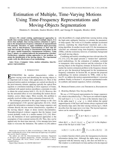
982 IEEE TRANSACTIONS ON IMAGE PROCESSING, VOL. 17, NO. 6, JUNE 2008 

Estimation of Multiple, Time-Varying Motions 

Using Time-Frequency Representations and 

Moving-Objects Segmentation 

Dimitrios S. Alexiadis, Student Member, IEEE, and George D. Sergiadis, Member, IEEE 

Abstract—We extend existing spatiotemporal approaches to 

handle time-varying motions estimation of multiple objects. It is 

shown that multiple, time-varying motions estimation is equivalent 

to the instantaneous frequency estimation of superpositioned 

FM sinusoids. Therefore, we apply established signal processing 

tools, such as time-frequency representations to show that for 

each time instant, the energy is concentrated along planes in the 

3-D space: spatial frequencies—instantaneous frequency. Using 

fuzzy C-planes, we estimate indirectly the instantaneous velocities. 

Furthermore, adapting existing approaches to our problem, we 

attain the identification of the moving objects. The experimental 

results verify the effectiveness of our methodology. 

Index Terms—Computer vision, motion estimation, time-frequency 

representations. 

I. INTRODUCTION 

ESTIMATING the motion characteristics within a 

time-varying scene and identifying the moving objects is 

an important task in many video applications [1]. Most of the 

proposed motion analysis techniques are carried out directly in 

the pixel-intensity domain, applying typically the optical flow 

equation or correlation-matching in short sequences of frame, 

combined with spatial motion-smoothness constraints in order 

to obtain the actual motion field [1, Ch. 6]–[3]. However, this 

has the unwanted effect of over-smoothing the motion discontinuities, 

across object edges. More recently, this problem is 

partially resolved within a robust estimation framework [4]. 

The technique presented in this paper belongs to the class 

of spatiotemporal (3-D) spectral approaches [6]–[12], which 

exploit the information contained in long image sequences and 

estimate directly the true motion characteristics, regardless of 

the moving objects’ shape or dense motion discontinuities. 

Neurophysiological evidence suggests that the human visual 

system probably works in a similar manner [13], [14]. However, 

the limitation of most spatiotemporal approaches is the 

assumption of time-constant motion [6]–[9]. Thus, they can be 

applied only for short time intervals. A few attempts have been 

made to overcome the limitation. The authors in [10] address 

Manuscript received June 24, 2006; revised February 4, 2008. The associate 

editor coordinating the review of this manuscript and approving it for publication 

was Dr. Onur G. Guleryuz. 

The authors are with the Telecommunications Laboratory, Department 

of Electrical and Computer Engineering, Aristotle University of Thessaloniki, 

Thessaloniki GR 54124, Greece (e-mail: dalexiad@mri.ee.auth.gr; 

sergiadi@auth.gr). 

Digital Object Identifier 10.1109/TIP.2008.922437 

1057-7149/$25.00 © 2008 IEEE 

only the problem of a single global time-varying motion, using 

the high-order ambiguity function, to estimate the parameters 

of chirp signals. The work in [11] handles multiple accelerated 

motions, exploiting the chirp-Fourier transform and a clustering 

algorithm. In another recent work [12], the instantaneous 

velocities are estimated using time-frequency representations 

(TFRs), with the restriction, however, of stationary background 

and small moving objects. 

Combining and mainly extending previous relevant ideas [6], 

[7], [11], [12], this paper presents a “motion first” spatiotemporal 

methodology, for the estimation of multiple, occluded 

or transparent, time-varying motions and the extraction of the 

moving objects in the frequency domain. In Section II, we formulate 

the motion estimation problem in the frequency domain 

and we give the theoretical background for the instantaneous 

frequency estimation. In Section III, we present the proposed 

methodology for motion estimation by TFRs, while in Section 

IV, we address the motion segmentation/objects’ extraction 

problem. Finally, in Section V, we present experimental results 

on synthetic and natural sequences, before concluding. 

II. PROBLEM FORMULATION AND THEORETICAL BACKGROUND 

A. Modeling Multiple Time-Varying Motion 

We use a 2.5-D layered representation for image sequences 

[5], which is described in Fig. 1. The layers are ordered in depth. 

For each layer , we have a) the intensity map ; 

b) the alpha map , which defines the spatial 

support/opacity of the layer and remains always registered with 

the intensity map; and c) the time varying velocity , which 

describes how the maps move over time. The layered representation 

can be summarized in the equation 

where is the displacement 

of the th layer at time and 

is a window function which carries the transparency/occlusions 

information during time. Although the alpha map remains 

registered with the intensity map , this does not hold for . 

The window is deformed over time and has to be decomposed 

(1) 

(2)

ALEXIADIS AND SERGIADIS: ESTIMATION OF MULTIPLE, TIME-VARYING MOTIONS USING TIME-FREQUENCY REPRESENTATIONS 983 

Fig. 1. Block diagram for our layered model, similar to the one in [5]; “cmp” 

represents @— AaI0 — . 

into a constant portion and a deformable, error-introducing portion. 

After some manipulations [6] 

where corresponds to the virtual, constant part of 

. The distortion term accounts for the deformation 

of due to occlusions. Any other source of distortion 

(sensor noise, deviation from the motion model, etc.) can also be 

included. An explicit analysis in the frequency domain for the 

occlusion distortion term in the case of time-constant velocities 

and two moving objects can be found in [15]. Notice that our 

model intrinsically can handle generally transparent motions, 

with the occluded motion being only a special case, when is 

simply zero or unity. 

B. Velocity Estimation as Instantaneous Frequency Estimation 

Consider the spatial (2-D) Fourier transform of each frame. 

From (3) and with ,wehave 

where the instantaneous phase of the th component is 

Consequently, the corresponding instantaneous frequency is 

where stands for the instantaneous velocity 

of the th object, which is considered to be a continuous 

and smooth function of , as expected by the physic’s laws. From 

(4)–(6), one can conclude the following. 

1) For a fixed spatial frequency , the signal is a superposition 

of frequency modulated (FM) complex sinusoids 

with instantaneous frequencies . 

2) For a given time instant , the instantaneous frequency 

varies linearly with and . The triplets 

lie on a plane through the origin, 

(3) 

(4) 

(5) 

(6) 

whose direction depend on the instantaneous velocity at 

the instant . 

According to the first conclusion, a key component of our 

approach is the estimation of the instantaneous frequencies 

. For this purpose, one can exploit established signal 

processing tools, such as the time-frequency representations 

[16]–[18]. 

C. Smoothed Pseudo Wigner–Ville (SPWV) Distribution 

In this subsection, we briefly review the smoothed pseudo 

Wigner–Ville (SPWV) distribution, which is used in our experiments. 

For a detailed analysis on TFRs, the reader is referred 

to [16]–[18]. We drop the variable for notational simplicity. 

The SPWV distribution of is given by 

namely from the 2-D convolution of the well-known 

Wigner–Ville (WV) distribution 

with a separable 2-D smoothing kernel , 

where is the Fourier transform of an 1-D smoothing 

window . 

The WV distribution presents perfect localization along 

the instantaneous frequency for a single linear FM sinusoid. 

However, it presents emphatic interference terms in the case 

of multicomponent signals, which may be destructive in many 

applications. Fortunately, the interference terms have oscillatory 

nature and can, therefore, be attenuated by the smoothing 

operation with the kernel . Introducing separable 

smoothing actions allows us to control the smoothing in time 

and frequency freely and independently to each other. The 

wider the time (frequency) smoothing window, the more time 

(frequency) smoothing can be achieved. Also, it can be shown 

that the well-known spectrogram, namely the squared modulus 

of the windowed (short-time) FT, is related to the WV distribution, 

using an appropriate (nonseparable) kernel [16]. 

D. Extracting Information From Time-Frequency Images 

The simplest approach to extract the instantaneous frequencies 

is to find the peaks along in the TFR image, for 

each . However, in order to obtain robustness against noise and 

interference terms, we use the following methodology. Considering 

that the instantaneous velocities and, consequently, the instantaneous 

frequencies in (6) vary as smooth functions of 

, we expect smooth curves in the TF plane, which can be approximated 

as piecewise linear polynomials. Namely, one can 

approximate higher-order FM signals by piecewise linear FM 

signals. Let the length of the image sequence be . We break 

the interval into overlapping intervals of length 

(7) 

(8) 

(9)


where is the center time instant of the th interval . With 

being the overlapping factor between two successive 

intervals, we have 

(10) 

and . We want to estimate the mean 

frequencies and the chirp rates for each time interval. 

To its center , we assign the instantaneous frequencies estimations 

as . The instantaneous frequencies for each 

time instant can be interpolated from . For the desired 

estimations, we cut the TFR image into the overlapping 

time-slices , corresponding to the intervals 

. The linear FM estimation within 

each time interval is performed as described below. 

The WV distribution ideally maps a linear FM sinusoid into 

a line in the TF plane. Consequently, the problem of the detection-estimation 

of such a signal is reduced to the easy-to-solve 

problem of detecting a line, which can be accomplished using 

the Hough transform. Applying the Hough transform to the WV 

distribution, one obtains the Wigner–Hough transform [18]. It 

can be shown that this is the asymptotically efficient estimator 

(it reaches the Cramer–Rao bound) of linear FM sinusoids in 

white Gaussian noise. In practice the TFR is calculated for discrete 

values of and . Therefore, we use a discrete-space version 

of Hough transform, similarly to [9]. The distance between 

a point in a discrete image and a line 

with slope and bias is calculated by 

(11) 

A “digital” line of width is defined as the set of 

all satisfying . Given the total 

height of a TFR equal to , a good value for , that is used 

in our experiments is . The detection-estimation of 

lines is performed by searching the peaks of the 2-D function 

(line matched filter) 

(12) 

where is the number of pixels belonging to the line 

. Notice that, thanks to the integration along lines, 

even when strong interference-terms are present in the TFR images, 

they are attenuated because they have oscillatory nature. 

Therefore, the detector is relatively efficient for multiple FM 

components. 

III. PROPOSED METHODOLOGY 

A. General Approach 

According to the motion analysis of Section II and the theory 

of TFRs, a methodology for smoothly time-varying motions estimation, 

can be summarized in the following steps. 

1) For each spatial frequency , we map the 

signal into the TF plane using a TF representation 

(13) 

2) For each time interval (and each spatial frequency) the 

frequencies of the FM components are calculated 

using the methodology of Section II-D. 

3) For each time interval , we arrange the data as 3-D 

points 

(14) 

where is the number of data points. These triplets are expected 

to be concentrated along planes through the origin. 

Using the fuzzy C-planes (FCP) clustering algorithm as in 

[11], we group them into planes, calculating simultaneously 

the planes’ parameters and consequently the velocities 

, according to (6). The velocities 

for each time instant are interpolated from . 

The efficiency of the above approach depends strongly on the 

accuracy of the instantaneous frequencies estimates 

given at the second step. Exploiting the estimates for many 

spatial frequencies using clustering renders the methodology 

more efficient. 

B. Some Remarks and Implementation Details 

Static Background: The effect of a static background is the 

addition of a DC term in , for each spatial frequency [see 

(4)–(6)]. Therefore, for each one can subtract from its 

mean value. This cancels out the strong effects due to the static 

background in the TF plane and reveals the weaker frequency 

components. 

Temporal Aliasing: The minimum required sampling rate for 

an alias-free (smoothed pseudo-) WV distribution is twice the 

Nyquist rate. Therefore, aliasing introduces wrapping of the motion 

planes around , along the temporal frequency. As a 

consequence, it is preferred to feed the FCP clustering algorithm 

only with triplets corresponding to low spatial frequencies 

such that . Also, for small , 

the SNR remains high, since the natural images 

have their energy concentrated in low spatial frequencies, 

in contrast to the noise term. 

Spatially Local Application: The assumptions of the motion 

model may be relaxed, letting the objects (the intensity 

and alpha maps) deform slowly with time, because of the timewindowing 

introduced by the TF representations. This is verified 

also from the presented experimental results. Additionally, 

applying the motion model within spatial blocks (overlapping 

or not), more complicated motions (for example affine) 

are well approximated. Compared to pixel-domain approaches, 

frequency-domain approaches suffer from requiring large local 

windows, where different motions can occur. This problem is 

partly resolved given that our approach can handle discontinuous 

motions. 

TFR Windows Selection: The choice of the windows’ type 

and width used in TFRs affect the accuracy of the instantaneous 

frequencies estimations. However, the optimal width depends 

on the instantaneous frequencies, which are the unknowns to be 

estimated, as analyzed in [12]. An explicit study about the influence 

of the used windows to the accuracy of the proposed


method is beyond the scope of this paper, since the final velocity 

estimates depend on the effectiveness of the FCP. Notice, 

however, that for all the experiments presented, the methodology 

worked effectively using a discrete Hamming window of 

length as the time-smoothing window and a Hamming 

of length as the frequency-smoothing window 

, where is the length of the sequence. 

IV. MOVING OBJECTS’S EXTRACTION 

AND MOTION SEGMENTATION 

In order to complete our motion estimation task by additionally 

identifying the moving objects, we modify two known approaches 

[19]–[21] adapting them to our problem, as follows. 

A. Objects’s Extraction in the Frequency Domain 

Ignore the error term in (4) and define 

, which according to the analysis in Section II-A corresponds 

to the constant shape part of the th object, shifted 

by . Discretizing the time-variable, for each spatial frequency 

we have a linear system , near ( is 

dropped for notational simplicity) 

. 

. 

. 

. 

. 

. 

. 

. 

. 

(15) 

where and 

is the displacement from frame to frame 

. Since the time-varying velocities and, consequently, the 

corresponding displacements were estimated, the phases-matrix 

is known and the objective is to calculate the objects-vector 

. When ,wehavean system of linear 

equations, which is solved analytically: . 

However, one can exploit the information contained in a 

longer frame sequence, by using and 

solving the system in the least squares sense, i.e. minimizing 

. 

Calculating for each and applying IFT to one 

obtains the image of the th object at . In practice, we find convenient 

to solve the system only when all the singular values of 

are upper and lower bounded (for instance, by 0.1 and 10, 

respectively), in order to avoid singularities and obtain robustness 

against noise. The missing values of for some 

spatial frequencies can be estimated using trigonometric or simpler, 

less computationally expensive interpolation schemes. Finally, 

when only low spatial frequency components are used, 

noise filtering is achieved directly in the frequency domain. Obviously, 

an advantage of the described approach is that it can be 

directly applied for separating transparent objects. 

B. Segmentation by Energy Minimization 

The goal here is to assign to each pixel one of the estimated 

velocities, i.e., a motion label , introducing the 

Fig. 2. -expansion graph, given for an 1-D image for simplicity. The appropriate 

link weights are given in Table I. 

TABLE I 

WEIGHTS USED IN THE -EXPANSION ALGORITHM 

labeling , where is image plane. This 

is performed by searching for which minimizes the objective 

function (we drop for simplicity) 

(16) 

The objective term , given in (17), shown at the bottom 

of the next page, enforces the classification of the pixels based 

on the intensity residuals after motion compensation. This, however, 

becomes unreliable in the presence of noise or lack of 

texture. Therefore, also the spatial motion-smoothness term of 

(18), shown at the bottom of the next page, is used, with “ 

” meaning that is in the neighborhood of . The penalty 

is more tolerant in motion-labeling discontinuities 

when real intensity discontinuities are present. Also, the temporal 

smoothness term of (19), shown at the bottom of the next 

page, takes into account the labeling of previous frames. 

The optimal solution for the energy function of (16) can be 

obtained using the -expansion algorithm [20], [21], which is 

well suited to our problem, giving a very fast solution. Traditional 

optimization techniques (such as gradients, Hessians, 

etc.) cannot be applied here because is multimodal and 

nonconvex. Also, the application of genetic algorithm is computationally 

expensive, according to our experiments. The -expansion 

algorithm is summarized as follows. 

1) Initialization: Start with the labeling which simply 

minimizes , i.e. the motion residuals. 

2) Cycle: For each label : 

• Iterations: Find the optimal within an 

-expansion move, which is explained directly below. 

3) If , set and begin a 

new cycle, else finish.


Fig. 3. “White Tower & Boat”—frames 1, 32, and 64 (three first figures) and the extracted layers, obtained applying (20) to the objects’ images, taken using the 

proposed frequency-domain method, for the first 32 frames (last two figures). 

Fig. 4. “White Tower & Boat”—estimated instantaneous velocities. 

Fig. 5. “White Tower & Boat”—motion segmentation results using graph-cuts 

for the frames 1, 10, and 20. 

Given a label ,wehavean -expansion move if some labels 

in have changed to in . Dynamically in 

each iteration, a binary Graph is constructed as in Fig. 2. We 

have two terminal nodes and expressing whether a pixel 

will change its label to or not. The nonterminal nodes 

represent the image pixels. Two neighbor pixels , having 

different labels are connected through an intermediate auxiliary 

node with weights and . 

Neighbor pixels , with the same label are directly connected 

to each other with weights . The nonterminal 

nodes are connected to and with t-links of appropriate 

weights as in Fig. 2. With 

being the “data term” (see [20] for details), the weights used are 

with 

Fig. 6. “Walker”—walker’s positions in the frames 1, 11, 21, FFF, 181 of the 

natural sequence. 

Fig. 7. “Walker”—SPWV for 3 aHand (left) 3 aIS%aITH and (right) 

the estimated instantaneous velocity. 

summarized in Table I. In order to find the optimal -expansion 

move, we seek for the “minimum-cost” cut of the graph. A 

cut is a partitioning of the nodes into two subsets and 

such that and and it includes exactly one t-link 

for any pixel . Its cost is the sum of the weights of the links 

it includes. After finding the minimum-cost cut, a pixel is 

with (17) 

with 

otherwise 

otherwise 

(18) 

(19)


Fig. 8. “Transparent Lena-Cameraman”—frames 1, 16, and 32 of the sequence (first three figures) and the extracted layers using the proposed frequency-domain 

method (last two figures). 

Fig. 9. “Transparent Lena-Cameraman”—motion planes points @A for (left) 

w X P ‘IVY PT“ and (right) the estimated instantaneous velocities. 

assigned the label if the cut separates from the terminal , 

or it keeps its old label otherwise. 

C. Layers’ Synthesis, Background Mosaicing 

Given that the instantaneous velocities estimation was adequately 

precise and the moving objects were efficiently separated 

using one of the presented methodologies, the objects will 

appear stationary in the motion-compensated sequence. Variations 

due to occlusions, noise and illumination changes are expected. 

Moreover, some regions of a moving background appear 

only after some frames. The extraction of a complete representative 

image for each layer is performed by a temporal median 

operation [5] 

(20) 

where is the motion compensated-image of the th object. 

This procedure, together with the other layers, synthesizes 

the background mosaic (a panoramic image), or the “sprite” in 

MPEG-4 terminology. 

V. EXPERIMENTAL RESULTS 

The overall motion-estimation algorithm is described in Algorithm 

1 (shown at the top of the next page). The Matlab code 

that accomplishes the simulation results, described in this section, 

can be found at the web location: http://esopos.ee.auth.gr/ 

TIP-VaryingMotion/code.zip. In the first experiment, the spectrogram 

is used because of its simplicity. In the next experiments, 

the SPWV distribution is used, with a Hamming window 

of length as the time-smoothing window and a Hamming 

of length as the frequency-smoothing window 

. 

A. “White Tower & Boat” Synthetic Sequence 

The synthetically generated sequence of Fig. 3 contains 

a moving object (boat) on a moving background (White 

Tower). The frame size is 296 296 and the sequence’s 

length is frames. The background moves with velocity 

pixel/frame and the boat decelerates according to 

pixels/frame. The simulated sequence was 

generated according to the presented motion model of (1) and 

(2) and Fig. 1. We used two 8-bit grayscale still images, a background 

“White Tower” image of size 502 296 and an image 

containing the “Boat” object. These still images correspond to 

, 1, 2 of the model. The motion of the background 

was obtained by selecting the appropriate 296 296 region 

of the corresponding still image, for each time instant. For the 

“Boat,” we created manually an auxiliary “mask” image, which 

corresponds to the window of (1). We cropped the 

“Boat” object from the still image and superimposed it on the 

background frame, at the appropriate instantaneous location. 

In order to handle noninteger instantaneous displacements, we 

applied bilinear interpolation. Finally, to obtain more natural 

visual appearance, we applied a weak smoothing operation near 

the border of the “Boat” object. 

For this experiment, White Gaussian Noise with 

dB was added. We use the spectrogram because of its 

simplicity. The window used to obtain the Short-Time Fourier 

Transform is a . In the TFR images, we search 

for two peaks along for each time instant . This is equivalent 

to applying the proposed Hough-transform methodology on 

TFR slices of length . Although, the spectrogram 

presents interference terms and bad localization, the estimated 

instantaneous velocities using FCP are very close to the 

real ones, as can be realized from Fig. 4. In Fig. 3, we also 

present the layers obtained applying (20) on the object images, 

obtained using the proposed frequency-domain approach of 

Section IV-A. Finally, in Fig. 5, we give results of the motion 

segmentation approach, using the graph-cuts. 

B. “Walker” 

The natural sequence, used in [12] and depicted in Fig. 6, contains 

a single walker, whose size is small compared to the static 

background. The sequence contains video-frames of 

size 320 240. The SPWV of for and a given 

value of is depicted in Fig. 7. The TFR images are clear in the 

sense that almost no interference terms exist and the TF localization 

is good. Applying our methodology by cutting the TFR 

images into overlapping time-slices of length 

with overlapping factor , the estimated instantaneous 

velocity is given in Fig. 7. Our results are similar to those in 

[12]. However, our methodology is more general in the sense 

that it can handle also sequences with large moving objects and 

moving background, at the cost of increased computational effort.


C. Transparent “Lena -Cameraman” Synthetic Sequence 

In order to verify the effectiveness of the approach for transparent 

motions, we created the synthetic sequence shown in 

Fig. 8. The final sequence shown is of size 256 256 and length 

. To generate it, we used 8-bit grayscale, 512 512 

versions of the well-known “Lena ” and “Cameraman” still images. 

The velocities of the sequence are nonzero only along the 

-direction. Therefore, along the -direction, we used only the 

region of the original images . 

The instantaneous horizontal velocities vary as quadratic polynomials 

of time, as depicted in Fig. 9. The motions of the 

layers were obtained by selecting the appropriate regions of the 

corresponding still images: (“Lena”) 

and (“Cameraman”), 

which are of size . The translating foreground 

“Lena ” layer is opaque except from a together-translating 

rectangular region, where it is transparent. According to the 

presented motion model, the corresponding “alpha” map is 

unity everywhere, except from the rectangular image region: 

(for the first frame), 

where it is equal to 0.5. To handle noninteger instantaneous 

displacements, we applied bilinear interpolation. 

White Gaussian noise (WGN) with dB was added. 

The estimated instantaneous velocities are given in Fig. 9, together 

with the actual ones. Using the SPWV, the estimated 

motion planes points for are also given in 

Fig. 9. Finally, using the presented frequency domain approach, 

the synthesized layers are presented in Fig. 8. 

D. Modified “Coast Guard” 

In this experiment, the well-known “Coast Guard” sequence 

is used. In order to have time-varying motion for the back- 

ground, we have created a modified sequence (depicted in 

Fig. 10) of length . The original sequence’s frames 

138–265 are used with an increasing rate, according to the 

formula: , with and being the 

frame numbers in the new and the original sequence, respectively. 

The SPWV for is given in Fig. 11(a). 

Notice that strong interference terms are present, because the 

applied time/frequency smoothing is not sufficient. However, 

applying the presented Hough-transform methodology, the 

estimation of the instantaneous frequencies becomes reliable. 

Two peaks are clearly visible in the output of the line matched 

filter [Fig. 11(c)] applied to the SPWV slice of Fig. 11(b). The 

length of the SPWV slices is and the overlapping 

factor between successive pieces . The estimated 

instantaneous velocities and displacements are given in Fig. 11 

which are close to the real ones, found by manual feature-point 

tracking. In Fig. 10, the extracted layers are also shown, using 

(20) on the results of the frequency-domain approach of Section 

IV-A. 

E. CAVIAR Sequence—Man Walking 

The proposed methodology was successfully applied also 

on sequences captured for the purpose of the CAVIAR project 

[22]. We present the results for the frames 310–437 of the 

original “Walk2” sequence captured at the INRIA-lab, with 

a time-downsampling factor equal to 2. The final sequence, 

depicted in Fig. 12, has frames of size 384 288 

and contains a man walking along a parabolic trajectory. 

For the piecewise linear approximation of the instantaneous 

frequencies curves, the produced TFR images were cut into 

overlapping slices of length , with overlapping factor 

. The final results are given in Fig. 13 and they are 

reasonably accurate, compared to the ground-truth values.


Fig. 10. Modified “Coast Guard” sequence—frames 1, 21, and 41 (three first figures) and the extracted layers using the first 30 frames (last two figures). 

Fig. 11. Modified “Coast Guard”—from left to right: SPVW for @3 Y3 Aa@IQ%aIUTY HA, slice of the SPWV image for w X P ‘PWY RR“, and corresponding 

output of the line-matched filter. The estimated instantaneous velocities and displacements, compared to the real ones. 

Fig. 12. “CAVIAR”—frames 1, 31, and 61 of the natural sequence (first three figures) and (right) the extracted stationary-background and moving man objects 

for the 16th frame. 

Fig. 13. “CAVIAR”—estimated instantaneous velocity and displacement, compared to the real ones. 

Finally, in Fig. 12, we present results of the proposed frequency 

domain objects extraction method. 

VI. CONCLUSION 

Combining and extending previously published ideas [6], [7], 

[11], [12], we presented a new spatiotemporal approach for the 

estimation of the motions of multiple objects, which move with 

time-varying velocities. For this task, TFR was the appropriate, 

selected signal processing tool. We applied the Hough transform 

in overlapping time-slices of the TFR images to increase 

the robustness against noise and interference terms, present in 

the TFRs. Moreover, by exploiting the instantaneous frequencies 

estimates obtained for many spatial frequency pairs using 

FCP, we increased the robustness and accuracy of our method. 

Having estimated accurately the objects velocities, the proposed 

objects segmentation approaches produced correct and meaningful 

results. The experiments on various synthetic and natural 

sequences verified the effectiveness of the proposed method. 

The presented and used motion model considers time-varying 

but space-invariant motions and its effectiveness was demonstrated 

for the dominant and relatively large moving objects 

. However, by applying space-locally the proposed approach, 

namely using local (windowed) 2-D Fourier transforms, 

the above limitations no longer exist. This comes with increased 

computational effort, compared to constant motions approaches, 

but also with the benefit of increased accuracy. Our future research 

will focus on achieving real-time motion tracking characteristics, 

for both monochrome and color image sequences. 

REFERENCES 

[1] Y. Wang, J. Ostermann, and Y. Zhang, Video Processing and Communications. 

Englewood Cliffs, NJ: Prentice-Hall, 2002. 

[2] B. K. B. Horn and B. G. Schunck, “Determining optical flow,” Artif. 

Intell., vol. 17, pp. 185–203, 1981. 

[3] H. H. Nagel and E. Enklemann, “An investigation of smoothness constraints 

for the estimation of displacement vector fields from image sequences,” 

IEEE Trans. Pattern Anal. Mach. Intell., vol. PAMI-8, no. 9, 

pp. 565–593, Sep. 1986.


[4] M. J. Black and P. Anandan, “The robust estimation of multiple 

motions: Parametric and piecewise-smooth flow-fields,” Comput. Vis. 

Image Understand., vol. 63, pp. 75–104, Jan. 1996. 

[5] J. Y. A. Wang and E. H. Adelson, “Representing moving images with 

layers,” IEEE Trans. Image Process., vol. 3, no. 9, pp. 625–638, Sep. 

1984. 

[6] W.-G. Chen, G. B. Giannakis, and N. Nandhakumar, “A harmonic retrieval 

framework for discontinuous motion estimation,” IEEE Trans. 

Image Process., vol. 7, no. 9, pp. 1242–1257, Sep. 1998. 

[7] C. E. Erdem, G. Z. Karabulut, E. Y. Yanmaz, and E. Anarim, “Motion 

estimation in the frequency domain using fuzzy c-planes clustering,” 

IEEE Trans. Image Process., vol. 10, no. 12, pp. 1873–1879, Dec. 2001. 

[8] B. Porat and B. FriedLander, “A frequency domain algorithm for multiframe 

detection of Dim targets,” IEEE Trans. Pattern Anal. Mach. 

Intell., vol. 12, no. 4, pp. 398–401, Apr. 1990. 

[9] P. Milanfar, “Two-dimensional matched filtering for motion estimation,” 

IEEE Trans. Image Process., vol. 8, no. 3, pp. 438–444, Mar. 

1999. 

[10] W.-G. Chen, G. B. Giannakis, and N. Nandhakumar, “Spatiotemporal 

approach for time-varying global image motion estimation,” IEEE 

Trans. Image Process., vol. 5, no. 10, pp. 1448–1461, Oct. 1996. 

[11] D. S. Alexiadis and G. D. Sergiadis, “Estimation of multiple accelerated 

motions using chirp-Fourier transform and clustering,” IEEE 

Trans. Image Process., vol. 16, no. 1, pp. 142–152, Jan. 2007. 

[12] I. Djurovic and S. Stankovic, “Estimation of time-varying velocities of 

moving objects by time-frequency representations,” IEEE Trans. Image 

Process., vol. 12, no. 5, pp. 550–562, May 2003. 

[13] E. H. Adelson and H. R. Bergen, “Spatiotemporal energy models for 

the perception of motion,” J. Opt Soc. Amer. A, vol. 2, pp. 284–299, 

1985. 

[14] B. A. Watson and A. J. Ahumada, “Model of human visual-motion 

sensing,” J. Opt Soc. Amer. A, vol. 2, pp. 322–342, 1985. 

[15] S. S. Beauchemin and J. L. Barron, “The frequency structure of one-dimensional 

occluding image signals,” IEEE Trans. Pattern Anal. Mach. 

Intell., vol. 22, no. 2, pp. 200–206, Feb. 2000. 

[16] L. Cohen, “Time-frequency distributions: A review,” Proc. IEEE, vol. 

77, no. 7, pp. 941–981, Jul. 1989. 

[17] L. J. Stanckovic, “The auto-term representation by the reduced interference 

distributions; The procedure for a kernel design,” IEEE Trans. 

Signal Process., vol. 44, pp. 1557–1564, June 1996. 

[18] S. Barbarossa, “Analysis of multicomponent LFM signals by a combined 

Wigner-Hough transform,” IEEE Trans. Signal Process., vol. 43, 

no. 6, pp. 1511–1515, Jun. 1995. 

[19] C. Mota, I. Stuke, T. Aach, and E. Barth, “Divide-and-conquer strategies 

for estimating multiple transparent motions,” in Lecture Notes on 

Computer Science. Berlin, Germany: Springer, 2005, vol. 3417. 

[20] Y. Boykov, O. Veksler, and R. Zabih, “Fast approximate energy minimization 

via graph cuts,” IEEE Trans. Pattern Anal. Mach. Intell., vol. 

23, no. 11, pp. 1222–1239, Nov. 2001. 

[21] V. Kolmogorov and R. Zabih, “What energy functions can be minimized 

via graph cuts?,” IEEE Trans. Pattern Anal. Mach. Intell., vol. 

26, no. 2, pp. 147–159, Feb. 2004. 

[22] 2005, The CAVIAR website [Online]. Available: http://homepages.inf.ed.ac.uk/rbf/CAVIAR/ 

Dimitrios S. Alexiadis (S’03) was born in Kozani, 

Greece, in 1978. He received the Diploma degree 

in electrical and computer engineering from the 

Aristotle University of Thessaloniki, Thessaloniki, 

Greece, in 2002. He is currently pursuing the Ph.D. 

degree at the Telecommunications Laboratory, Department 

of Electrical and Computer Engineering, 

Aristotle University of Thessaloniki. 

Since 2002, he has been involved in several research 

projects and, at the same time, he was a Research 

and Teaching Assistant at the Aristotle University. 

His main research interests include image/video processing and speech 

synthesis/recognition. 

Mr. Alexiadis is a member of the Technical Chamber of Greece. 

George D. Sergiadis (M’88) was born in Thessaloniki, 

Greece, in 1955. He received the Diploma in 

Electrical Engineering from the Aristotle University 

of Thessaloniki in 1978 and the Ph.D. degree from 

the Ecole Nationale Supérieure des Télécommunications, 

Paris, France, in 1982. 

He was with Thomson CsF, France, until 1985, 

participating in the development of the French 

Magnetic Resonance Scanner. Since 1985, he has 

been with the Aristotle University of Thessaloniki, 

teaching telecommunications and biomedical engineering, 

now as a Full Professor. For three years, he also served as the 

Director of the Telecommunications Department. He has developed the Hellenic 

TTS engine “Esopos” and designed the mobile communications for the 

Athens Olympic Games in 2004. His current research interests include fuzzy 

image processing and wireless communications. During the academic year 

2004–2005, he was a Visiting Researcher at the Media Lab, Massachusetts 

Institute of Technology, Cambridge. 

Dr. Sergiadis is the President of ELEVIT, the Hellenic society for Biomedical 

Engineering, and a member of TEE, ATLAS, SMRM, ESMRM, EMBS, and 

SCIP.

Estimation of Multiple, Time-Varying Motions Using ... - IEEE Xplore

Create successful ePaper yourself

Delete template?

Save as template?