Estimation of additive and dominance genetic variances for - CGIL ...

More documents

Recommendations

Info

384 1. Introduction ( ) M.J.R. Pante et al.rAquaculture 204 2002 383–392 Breeding programs are designed to change the genetics of a population to improve its productivity and profitability. In animal breeding, a considerable amount of genetic progress has been achieved through the exploitation of the simple additive genetic effects. Non-additive genetic components such as dominance and epistatic effects are usually ignored because they tend to be confounded with the common maternal environment; they have little practical application in selection Ž Mrode, 1996 . , and their estimation would involve large computational requirements Ž Varona and Misztal, 1999 . . However, accounting for non-additive genetic effects in genetic evaluation models is important for obtaining accurate predictions of breeding values of animals, to obtain a precise estimate of heritability and precise prediction of response to selection, and to help in deciding which breeding strategy and selection method should be utilized. There is a renewed interest in the estimation of non-additive genetic effects for important traits in domesticated animal species. This was set off by the improvement in computing facilities and availability of software ŽMeyer, 1989; Hoeschele and Van Raden, 1991; Misztal, 1997. that permit estimation of non-additive genetic effects from large field data sets. Evidence of non-additive genetic variation for important traits has been reported in cattle ŽHoeschele, 1991; Tempelman and Burnside, 1991; Fuerst and Solkner, 1994; Miglior et al., 1995; Rodriguez-Almeida et al., 1995; Misztal, 1997; Misztal et al., 1997. and poultry ŽWei and van der Werf, 1993; Misztal and Besbes, 2000 . . In fish, salmonids in particular, several studies suggest a significant and important influence of non-additive genetic effects on growth traits. In a majority of these studies, the presence of non-additive genetic effects was based on the observation of a larger dam than sire component of variance when estimated using a nested mating design Ž Gjedrem, 1983; Gall and Huang, 1988; Gjerde and Schaeffer, 1989. or by the presence of a significant sire by dam interaction Ž Gunnes and Gjedrem, 1981; McKay et al., 1986. when estimated using a factorial design. However, the dam component in the above studies may be inflated by effects common to full-sibs other than additive and non-additive genetics, i.e. common environmental and maternal effects. Gall Ž 1975. found evidence of non-additive genetic variation for post-spawning body weight among crosses and backcrosses in two strains of rainbow trout. In rainbow trout, evidence of non-additive genetic effects is also seen by a significant inbreeding depression on growth Ž Pante et al., 2001a . , and significant heterosis when crossing inbred lines Ž Gjerde, 1988 . . However, low heterosis was found when crosses were performed between wild strains of Atlantic salmon Ž Gjerde and Refstie, 1984 . . In studies that estimated the dominance genetic variance for important traits in fish, results indicate that its magnitude is within the range of the additive genetic variance. For example, in chinook salmon, the dominance variance for freshwater and saltwater weights were 0.26 and 0.08, respectively Ž Winkelman and Peterson, 1994a . . For body weight after 9 and 22 months of saltwater rearing, estimated dominance variance were 0.19 and 0.27, respectively Ž Winkelman and Peterson, 1994b . . In Atlantic salmon, the dominance variance for body weight at harvest ranged from 0.02 to 0.18 depending on the models utilized Ž Rye and Mao, 1998 . . These estimates imply that dominance is an
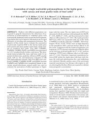
( ) M.J.R. Pante et al.rAquaculture 204 2002 383–392 385 important source of genetic variation for some growth traits in fish. Therefore, the purpose of this study was to determine the magnitude of additive and dominance genetic variances for body weight at harvest of rainbow trout and the common environmental effect due to full-sib groups. 2. Materials and methods Data were from three rainbow trout populations under selection for six generations at the Aqua Gen AS in Norway from 1972 to 1992. Each population was established separately in a different year Ž Table 1 . . The founding individuals for each population were from different fish farms in Norway and Sweden and thus were assumed to be from different gene pools. The pedigree data comprised seven generations Žgenerations 0–6 . . Individual growth was measured as body weight Ž kg. at harvest recorded after 16–18 months of rearing in floating net cages in the sea. The data analyzed were from generations 2–6 for all three populations and comprise a total of 15 year-classes Ž Table 1. and with a data structure as presented in Table 2. The fish were offspring of broodstock selected mainly for fast growth rate, and the selection method practiced was a combination of between-family and within-family selection. A hierarchical mating design was applied where each sire is mated on average to two to three dams. In all generations, full- and half-sib matings were avoided and matings that would yield inbreeding coefficients of 12.5% or higher were restricted. Marking of newly hatched larvae or fry is impossible; thus, each full-sib family was reared in separate tanks until reaching the average tagging size of 20 g. This introduces an environmental effect common to full-sib groups. To identify the families, a combination of fin clipping and freeze-branding was used Ž Gunnes and Refstie, 1980 . . The individuals selected as parents for the next generation were individually marked with operculum tags. Variance components for body weight at harvest were estimated for different effects fitted to a single trait animal model using the AIREMLF90 program ŽTsuruta and Misztal, 2000 . . The algorithm uses the Average Information Ž AI. as second differentials Table 1 The three separate populations analyzed in the study and the year-classes representing the time of hatching in each population Generation Population 1 Population 2 Population 3 0 1972 1973 1974 a 1 1975 1976 1977 2 1978 1979 1980 3 1981 1982 1983 4 1984 1985 1986 5 1987 1988 1989 6 1990 1991 1992 a The first generation where offspring were selected for fast growth rate.
Page 1: Ž . Aquaculture 204 2002 383-392 w
Page 5 and 6: ( ) M.J.R. Pante et al.rAquaculture

Estimation of additive and dominance genetic variances for - CGIL ...

You also want an ePaper? Increase the reach of your titles

Delete template?

Save as template?