High Energy X-ray Diffraction Microscopy (HEDM) - Materials ...
High Energy X-ray Diffraction Microscopy (HEDM) - Materials ...
High Energy X-ray Diffraction Microscopy (HEDM) - Materials ...

Create successful ePaper yourself
Turn your PDF publications into a flip-book with our unique Google optimized e-Paper software.
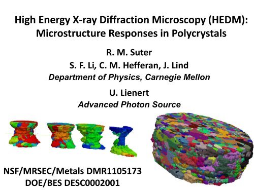
<strong>High</strong> <strong>Energy</strong> X-<strong>ray</strong> <strong>Diffraction</strong> <strong>Microscopy</strong> (<strong>HEDM</strong>):<br />
Microstructure Responses in Polycrystals<br />
R. M. Suter<br />
S. F. Li, C. M. Hefferan, J. Lind<br />
Department of Physics, Carnegie Mellon<br />
U. Lienert<br />
Advanced Photon Source<br />
NSF/MRSEC/Metals DMR1105173<br />
DOE/BES DESC0002001
What’s different about x-<strong>ray</strong> orientation mapping?<br />
Carnegie<br />
Mellon<br />
MRSEC<br />
Non-destructive<br />
Inside of bulk material<br />
Watch bulk material respond to stimuli
Outline<br />
1. Synchrotron radiation sources<br />
2. Near-field <strong>HEDM</strong> principles and practice<br />
3. Validation<br />
4. Orientation gradients<br />
5. Misorientations: angles and axes<br />
6. Combining with far-field
X-<strong>ray</strong> Absorption Lengths in Elemental Solids<br />
• 50 keV – 100 keV well matched to transmission through<br />
mm sized samples<br />
• Comparable to beam sizes 30 m downstream from source
<strong>HEDM</strong> Common Feature:<br />
Bragg Scattering at <strong>High</strong> <strong>Energy</strong><br />
All scattering vectors with c > q<br />
can be observed<br />
With a single rotation, we can access large region of reciprocal space
APS 1-ID <strong>High</strong> <strong>Energy</strong><br />
Beamline<br />
ESRF ID-11 <strong>Materials</strong><br />
Science Beamline<br />
Third Generation Synchrotron<br />
Radiation Sources<br />
• Small source size<br />
• <strong>High</strong> energy<br />
• Insertion devices<br />
Petra III P07 The <strong>High</strong> <strong>Energy</strong><br />
<strong>Materials</strong> Science Beamline
Magnetic Lattices as Sources<br />
Wiggler:<br />
I ~ N<br />
Broad spectrum<br />
Undulator:<br />
I ~ N 2<br />
Peaked spectrum
APS Undulator
Undulator X-<strong>ray</strong> Source
APS-U @ 1-ID: sources<br />
R. Dejus<br />
Request canted undulators:<br />
(i) superconducting (fixed<br />
period w/3 rd harmonic<br />
~70keV)<br />
(ii) revolver PM (2.3&2.5cm)<br />
for continuous coverage<br />
Request a long straight section<br />
to accommodate undulators &<br />
maximize length<br />
Heat loads more tolerable with<br />
short-period devices<br />
* 1.6cm SCU 300kW/mrad2 at<br />
min gap 9mm<br />
Advanced Photon Source 11
Specialized beam line requirements<br />
~2 m<br />
APS 1-ID beam line optics
Near-field <strong>HEDM</strong>: Orientation Field Mapping<br />
Apparatus at 1-ID at APS<br />
• Monochromatic x-<strong>ray</strong>s (> 50keV)<br />
• 1 – 5 mm beam height<br />
• 1.3 mm beam width<br />
• Air bearing rotation<br />
• 1.5 mm detector pixels<br />
• L = 4 – 12 mm<br />
Meaurement resolutions<br />
• Spatial: 1 - 4 mm<br />
• Orientation resolution: ~ 0.1 degree<br />
• Elastic strain: ??<br />
• Time: ~10 layers/hour<br />
Image diffracted beams<br />
from planar grain crosssections<br />
during 180<br />
degree w rotation<br />
in dw integration intervals<br />
• Lienert et al, JOM 2011<br />
• Suter et al, Eng Mat &<br />
• Tech 2007<br />
• Suter et al, RSI 2006<br />
• H.F. Poulsen, Springer<br />
Tracts, 2004
June 2012: Commissioning of new camera & mount<br />
Ulrich Lienert & Erika Benda<br />
• Increased stability<br />
• Simplified/smaller snout<br />
• Continuous rotation and<br />
synchronized readout of<br />
CCD
<strong>HEDM</strong>: Forward Modeling Orientation Field Reconstruction<br />
100 – 150 Braggs per grid element<br />
• Shortcut algorithms: 4 – 100X speedup<br />
• Reconstructions during measurements<br />
• Computer simulation mimics<br />
experiment<br />
• ~10 5 voxels/layer<br />
• ~100 layers<br />
• Potentially ~10 7 orientations<br />
resolved per voxel<br />
• Parallel processing:<br />
CMU, APS clusters, NSF TeraGrid
Data Flow
Initial image analysis<br />
Simple thresholding Laplacian edge detection
Geometry Determination<br />
1. Center 30 micron gold wire (absorption imaging)<br />
2. Collect 3L data set from one layer<br />
3. Back project peaks to locate rotation axis distances<br />
4. Reconstruct using IceNine<br />
5. Monte Carlo on geometry parameters: L’s, (j0, k0)’s,…<br />
• In principle, these parameters should be fixed<br />
• Mechanical drifts (or bumps) occur<br />
• Volume measurement macros use 3L layers every ~50<br />
layers, 2L’s otherwise for speed<br />
• Degradation of reconstructions leads to additional p-MC
Calibration and Validation<br />
• 152(2) micron diameter Ruby sphere<br />
(NIST calibration standard)<br />
• Locate by absorption<br />
• 20 micron gold wire co-mounted
Near-field Reconstruction: <strong>High</strong> purity nickel<br />
One of 42 layer sections,<br />
0.156 mm 3 volume<br />
• ~400 grains/layer<br />
• ~45 mm ave diameter<br />
• Smallest grains 10 mm<br />
Black lines: mesh element<br />
neighbors with > 0.1 deg<br />
misorientation<br />
• Sample has well ordered grains<br />
• ~0.1 deg experimental orientation resolution<br />
Grid elements generate ~100 relevant<br />
Bragg peaks<br />
Carnegie<br />
Mellon<br />
MRSEC<br />
20
Zirconium<br />
S0: initial state<br />
Narrowest cross-section<br />
Confidence delineation of grains:<br />
thresholding is just right!<br />
Note: “Confidence” is not a good statistical metric!
Technique Verification: <strong>HEDM</strong> & EBSD<br />
<strong>High</strong> purity nickel (1 mm diameter cylinder)<br />
EBSD <strong>HEDM</strong><br />
EBSD<br />
<strong>HEDM</strong>
Technique Verification: <strong>HEDM</strong> & EBSD<br />
• Compare distance in orientation space (misorientation)<br />
between coincident points in maps<br />
• Measured regions are not identical (planar x-<strong>ray</strong> beam vs<br />
polished surface)<br />
Point-to-point<br />
misorientation map<br />
°
NIST Single Crystal (?) Ruby Sphere<br />
• 152 micron diameter<br />
• Spherical to +/- 2 microns<br />
• 15 layers, 10 microns<br />
:<br />
0.28 deg about (0.2, -0.9, 0.4)<br />
Thanks to Joel Bernier<br />
Diffractometer Rocking Curve<br />
(0,-3,0) Bragg peak<br />
0.12 deg separation<br />
0.01 deg widths
Origin of intra-granular orientation resolution<br />
• Orientation search attempts to put 100 – 150 Bragg<br />
peaks in w-bins where they are observed<br />
• Small lattice rotations shift a subset to different bins<br />
w1 w2<br />
“Perfect” grain<br />
Detector image of a diffraction “spot”<br />
w1<br />
w2<br />
“Deformed” grain<br />
• Deformation generates broadening in both w and h at G hkl<br />
• Different G hkl’s sample a specific rotation differently<br />
Reasonable to expect sensitivity to / resolution of intra-granular<br />
orientation distributions
Simulation of a small grain<br />
with orientation gradient<br />
Five micron FCC grain<br />
Simulate with 384 area element triangles<br />
+/- 5 degree rotation around <br />
(2 -2 -4) Bragg unaffected<br />
(1 -1 1), (2 2 0) maximally broadened
w = -13.5 +/- 0.5 deg
w Lineshapes<br />
w = 93 94 95 96 97 98 99 100 deg deg
Reconstruction compared to broadened scattering<br />
w24<br />
Cu in<br />
tensile<br />
strain
Reconstruction compared to broadened scattering<br />
w25<br />
Cu in<br />
tensile<br />
strain
Reconstruction compared to broadened scattering<br />
w26<br />
Cu in<br />
tensile<br />
strain
Reconstruction compared to broadened scattering<br />
w27<br />
Cu in<br />
tensile<br />
strain
Reconstruction compared to broadened scattering<br />
w28<br />
Cu in<br />
tensile<br />
strain
Simulation Validation
INTRA-GRANULAR ORIENTATION GRADIENTS: HP AL<br />
Misorientation Map<br />
4 deg color scale<br />
2 deg boundaries<br />
<strong>High</strong> Purity Al<br />
orientation changes<br />
located at boundaries
Statistics extraction from large data sets<br />
Neighbor<br />
misorientation<br />
angle<br />
distribution
Statistics extraction from large data sets<br />
Neighbor<br />
misorientation<br />
angle<br />
distribution<br />
S27a<br />
S27b S7 S3
Misorientation axes: Ni(Bi)<br />
Red lines = 0.1 degree from nominal sigma-axes
Post-Mortem With <strong>HEDM</strong><br />
Fracture surface (tomography) of Ni<br />
superalloy<br />
Orientation map 200 microns below<br />
the tip of the sample
Near-field <strong>HEDM</strong>: Technique Summary<br />
• Non-destructive 3D crystallographic orientation field mapping<br />
• Ordered and deformed materials: metals, ceramics, …<br />
• Opportunity for basic and applied work (or “basic work on applied<br />
materials”)<br />
• Large data sets for computational model comparisons<br />
• Tracking of materials responses<br />
• Thermal / mechanical / radiation / …<br />
• APS Upgrade (aps.anl.gov/Upgrade) implications<br />
• 1-ID beamline on the “fast track”<br />
• Improved beam stability<br />
• Superconducting undulator source – 10X in brilliance!<br />
• New end-station hutch currently being instrumented<br />
• Second, fixed high energy, undulator beamline: a dedicated instrument???<br />
• Easily combined with high energy tomography<br />
• Sample shape evolution<br />
• Crack / void formation and tracking<br />
• Easily (!) combined with far-field strain sensitive measurements
Near-field <strong>HEDM</strong>: Technique Summary<br />
• Compared to 3D EBSD<br />
• <strong>High</strong>er orientation resolution<br />
• Lower spatial resolution<br />
• Faster: 3D volumes in < 24 hours (will accelerate)<br />
• But, you need a synchrotron – and not just any!<br />
• Compared to DAXM<br />
• Comparable orientation resolution<br />
• Lower spatial resolution / lower strain resolution<br />
• Faster per volume<br />
• Millimeter samples in transmission<br />
• Compared to DCT<br />
• Comparable resolutions<br />
• Slower<br />
• Access to deformed structures<br />
• Compared to tomography<br />
• Measures three parameter orientation field rather than scalar<br />
density field
Far-field measurements: Elastic Strain States<br />
• M. Miller (Cornell), U. Lienert (APS 1-ID)<br />
• Risoe group<br />
Detector A: strain<br />
sensitivity at L ~ 1m<br />
Detector B: high<br />
resolution reciprocal<br />
space mapping at<br />
L ~ 5m<br />
Use fast, efficient<br />
medical imaging<br />
detectors<br />
Lienert et al, Risoe 2010 symposium proceedings<br />
Lienert et al, JOM 2011
Ti-6Al: in-situ straining with single grain resolved strain