Evaluating automated trading systems using random walk securities

Evaluating automated trading systems using random
walk securities
Tomoyasu Oya 1
1 Department of Computer Science and Engineering, Waseda University, Tokyo, Japan
Abstract - Evaluating automated trading systems (using
technical analysis) is sometimes difficult because of curvefitting,
survivorship bias, etc. In this paper, we report our
use of random walk stocks (GARCH (1, 1) model) to
evaluate automated trading systems. We created three
conditions: an uptrend market, a downtrend market, and an
oscillating market generating 10000 paths using the
GARCH model. We applied the simple strategies using
technical analysis to the random walk securities as future
stock prices. We observed the approximate characteristics
of the automated trading system in the three conditions.
This approach has a possibility to evaluate the automated
trading systems in the same scale regardless of the
complexity of the algorithms.
Keywords: random walk, automated trading, technical
analysis, investment science, GARCH model, VaR (Value at
Risk)
1 Introduction
Determining the usefulness of automated trading
systems is difficult because of curve-fitting, survivorship
bias, etc. Backtesting is a common way of evaluating these
trading systems. However, they do not always work because
past market prices differ from future ones.
Past stock prices are about as natural to use as
backtesting. Backtesting describes the past performance of
the automated trading system well. Frequently, the best
strategy is defined as one that performed the best in
backtesting. However, using that strategy does not always
work in actual future trading. Also, curve-fitting is a major
problem in backtesting. Determining which strategies overfit
is difficult.
Thus, we created random-walk securities as virtual
future stocks. In actual global markets, some researches
[5][6] refer to the randomness of the stock markets these
days. Creating an uptrend market, an oscillating market, and
a downtrend market enabled us to get hold of the
performance and the characteristics in automated trading
(using technical analysis). An automated trading algorithm is
like a black box when it is collected publicly (A Kaburobo
contest [1] is a competition of automated trading algorithms
between programmers). Using only backtesting based on
past stock prices seems insufficient as an evaluation tool.
We determined the approximate performance of
automated trading systems by using random walk securities
for the uptrend, oscillating, and downtrend markets.
2 Generating the random walk securities
system
We created paths using GARCH (1, 1) models. This
method is similar to the Monte Carlo simulation of value at
risk (VaR)[2]. In order to check the usefulness of technical
analysis, GARCH model or other stochastic models were
used[4][7].We used the prices of the Softbank Company in
2006-2007 as sample data. We divided the paths into
uptrend, oscillating, and downtrend markets, and we
backtested some algorithms using the securities in the
Kaburobo platform (written in JAVA ).
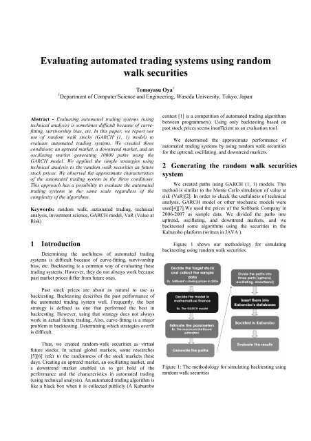
Figure 1 shows our methodology for simulating
backtesting using random walk securities.
Figure 1: The methodology for simulating backtesting using
random walk securities

3 Kaburobo platform
Kaburobo SDK is a programming tool for automated
trading systems. This is easy to create the algorithm based
on technical analysis (Ex. RSI, MACD, Bollinger band,
Moving average, etc.) and easy to backtest. We can also
manage the portfolio of the algorithm using the Kaburobo
SDK.
4 GARCH model
We chose the GARCH model. GARCH stands for the
generalized autoregressive conditional heteroscedasticity,
and the model is one approach to modeling a time series with
heteroscedastic errors. This model was proposed by Engle
(1982).
The GARCH model describes volatility clustering, which
refers to the observation "large changes tend to be followed
by large changes, of either sign, and small changes tend to be
followed by small changes." Volatility clustering is often
observed in the stock market. The GARCH model
parameters are often estimated using the maximum
likelihood estimation.
R = µ + ε
(1)
t
t
ε = σ ( σ > 0,
z is i.
i.
d(
0,
1))
(2)
t
t zt t t
=
p
∑ i t−i
q
∑ j t−
j
j i
i=
1
j=
1
2
2
2
σ ω + β σ + α ε ( ω > 0,
α , β ≥ 0)
(3)
t
The GARCH (p, q) model is described in the above
equations where t R is the return and µ t is the drift and ε t is
the innovation and σ t is the volatility. To simplify
estimating the parameters, we chose the GARCH (1, 1)
model. We chose a normal distribution for this study. A
Student's t-distribution is sometimes applied for describing
the fat tail distribution observed in the stock market. GJR
and EGARCH models are also used.
We selected the GARCH (1, 1) model and estimated its
parameters using the maximum likelihood estimation. We
used the prices of the Softbank Company in 2006-2007 as
the sample data.
5 Pre-estimating
First of all, does the GARCH (1, 1) model represent the
prices of the real market?
We determined using a statistical method whether the sample
data (the Softbank prices in 2006-2007) were appropriate for
the GARCH (1, 1) model.
5.1 Ljung-Box-Pierce Q test
A Ljung-Box-Pierce Q test determines whether any of a
group of autocorrelations of a time series differs from zero.
The result was that when the lag was 2, 5, 10, 15, or 20
(daily basis), the autocorrelations of a time series were
almost zero.
t
5.2 Engle's arch test
This test provided evidence supporting the GARCH effects
(i.e., heteroscedasticity). We checked whether residuals have
volatility clustering. The results were that GARCH effects
were evident when the lag was 2, 5, and 10 but not when the
lag was 15 or 20.
These tests were implemented by MATLAB[3]. The pvalue
was 0.05.
These results provide what might be a good reason to use
the GARCH model, and the sample data seems sufficient for
the GARCH model.
6 Estimating parameters
We then estimated the parameters using the maximum
likelihood estimation.
The estimated parameters are the following.
µ = 0.0001103, ω =0.00028359, β 1 =0.36043,
α 1 =0.20118
7 Creating the paths
We simulated the sample paths using the aforementioned
estimated parameters on a daily basis. Figure 2 shows the
paths were replicated 50 times. We created 10000 paths and
divided them into three parts. The upper part of one third of
the observed paths was defined as the uptrend market. The
middle part of one third of the observed paths was defined as
the oscillating market. The lower part of one third of the
observed paths was defined as the downtrend market.
Figure 2 : Generating the paths (replicated 50 times)
8 The strategies
We created seven kinds of strategies. These strategies
consist of the following trends, and the contrarian includes
short selling.
Here are the strategies:
1. When the RSI (10 days) < 30, they enter, when the RSI
(10 days) > 70 they exit. (contrarian)(The strategy 1.)

2. When the RSI (10 days) > 70, they enter, when the RSI
(10 days) < 30 they exit. (trend following) (The strategy
2.)
3. When the prices are down for 4 consecutive days, they
enter, when the prices are up for 4 consecutive days,
they exit. (contrarian)(The strategy 3.)
4. When the prices are up for 4 consecutive days, they
enter, when the prices are down for 4 consecutive days,
they exit. (trend following) (The strategy 4.)
5. When the RSI (10 days) < 30, they enter, when the RSI
(10 days) > 70 they exit. (short selling, trend following)
(The strategy 5.)
6. When the RSI (10 days) < 30, they enter, when the RSI
(10 days) > 70 they exit. (reversal, trend following) (The
strategy 6.)
7. When the moving average (5 days) < the moving
average (14 days)*0.96, they enter, when the moving
average (5 days) > the moving average (25 days)*1.04,
they exit (reversal) (The strategy 7.)
* RSI = Average of the closes on up days/ (Average of the
closes on up days + Average of closes on down days)*100
Strategy 6 and Strategy 7 are a bit complicated. Reversal
trading involves the following strategy: When investors have
stocks (a long position) and they have a sell signal, they sell
the stocks and start short selling at the same time. When they
have a short position and they have a buy signal, they buy
stocks back and start to have a long position.
9 The conditions of the strategies
The commission rate is 0.1% a trade. They spend half of the
money on one trade. They are allowed to buy extra positions
when they have another signal. They have an initial amount
of 50,000,000 yen. The initial price of the stock is 2,500 yen.
frequency
0.4
0.35
0.3
0.25
0.2
0.15
0.1
0.05
Buy and hold
-100 -50
0
0
-0.05
50 100 150
profit(%)
Figure 3 : Buy and hold
uptrend
downtrend
oscillating
frequency
0.3
0.25
0.2
0.15
0.1
0.05
-0.05
RSI contrarian
0
-100 -50 0 50 100 150
Figure 4 : RSI contrarian
frequency
0.35
0.3
0.25
0.2
0.15
0.1
0.05
profit(%)
RSI trend following
-100 -50
0
0
-0.05
50 100 150
profit(%)
Figure 5 : RSI trend following
frequency
0.35
0.3
0.25
0.2
0.15
0.1
0.05
Contrarian(4 days)
-100 -50
0
0
-0.05
50 100 150
profit(%)
Figure 6 : Contrarian (4 days)
frequency
0.35
0.3
0.25
0.2
0.15
0.1
0.05
Trend following (4days)
-100 -50
0
0
-0.05
50 100 150
profit(%)
Figure 7 : Trend following (4 days)
uptrend
oscillating
downtrend
uptrend
downtrend
oscillating
uptrend
downtrend
oscillating
uptrend
downtrend
oscillating

frequency
0.35
0.25
0.15
0.05
RSI trend following (short selling only)
0.3
0.2
0.1
0
-100 -50 0 50 100 150
-0.05
profit(%)
Figure 8 : RSI trend following (short selling only)
frequency
0.2
0.18
0.16
0.14
0.12
0.1
0.08
0.06
0.04
0.02
Reversal 1
-100 -50
0
-0.02
0 50 100 150
profit(%)
Figure 9 : Reversal 1.
frequency
0.8
0.7
0.6
0.5
0.4
0.3
0.2
0.1
Reversal 2
-100 -50
0
-0.1 0 50 100 150
profit(%)
Figure 10 : Reversal 2.
uptrend
downtrend
oscillating
uptrend
downtrend
oscillating
uptrend
downtrend
oscillating
Table 1 : The annual average returns and standard deviations
The strategy 1. Average Standard
return(%) deviation(%)
Uptrend 6.34 7.47
Oscillating 0.88 7.30
Downtrend -7.85 8.76
The strategy 2. Average Standard
return(%) deviation(%)
Uptrend 8.24 11.44
Oscillating -1.87 7.42
Downtrend -7.01 6.69
The strategy 3. Average Standard
return(%) deviation(%)
Uptrend 5.46 7.16
Oscillating -0.19 6.98
Downtrend -7.53 7.99
The strategy 4. Average Standard
return(%) deviation(%)
Uptrend 6.43 9.84
Oscillating -1.77 7.08
Downtrend -7.40 6.63
The strategy 5. Average Standard
return(%) deviation(%)
Uptrend -7.36 6.76
Oscillating -2.66 7.08
Downtrending 5.92 9.51
The strategy 6. Average Standard
return(%) deviation(%)
Uptrend 0.78 14.68
Oscillating -4.14 12.43
Downtrending 0.94 13.11
The strategy 7. Average Standard
return(%) deviation(%)
Uptrend 0.23 9.51
Oscillating -2.20 6.22
Downtrending 1.13 8.04
10 Experimental results
The annual returns and volatilities were shown in Table1.
The seven graphs show the results of each algorithm.
1. RSI contrarian(The strategy 1.)
2. RSI trend following(The strategy 2.)
3. Contrarian (4 days) (The strategy 3.)
4. Trend following (4 days) (The strategy 4.)
5. RSI contrarian (short selling only) (The strategy 5.)
6. Reversal 1. (The strategy 6.)
7. Reversal 2. (The strategy 7.)
These numbers are the same as the aforementioned
strategy.
First of all, we considered the RSI contrarian and RSI
trend following strategies. These strategies have a tendency
to link the profit with the original price itself. In short, if the
market is trending upwards, profit will likely increase. If the
market is trending downwards, profit will likely decrease.
We determined a similar situation in the contrarian (4 days)
and trend following (4 days) strategies.
The short selling strategies have a tendency for profit as
opposed to the market price; that is, if there is an uptrend
market, the profit likely decreases. If there is a downtrend
market, the profit likely increases.
These results seem natural. The profits are affected by the
original prices. The difference between the contrarian and
trend following strategies is small. A very simple technical
analysis does not seem superior to a buy and hold strategy in
the random walk market. But contrarian strategies and trend
following strategies seem to have the different kinds of the
distributions(We can see the difference of the standard
deviations in Table 1).
Now, let's consider the reversal strategies. These strategies
are complicated because they can frequently switch the long
and short positions. As a result, interestingly, the uptrend and
downtrend markets outperform the oscillating market. That is
not so easy to imagine even if we understand the algorithm.

Furthermore, the signal frequency affects the results. A
reversal 1 strategy generates buy and sell signals more
frequently than a reversal 2 strategy. Hence, we explain the
fact that the standard deviation of reversal 2 is smaller than
the reversal 1.
11 Conclusion
We observed the characteristics of automated trading
systems using random walk securities in uptrend, oscillating,
and downtrend markets. This approach can measure the
approximate risks and returns. Our system can evaluate the
algorithms written in technical analysis, no matter how
complicated they are in the same scale. This approach should
help in decisions making when creating and evaluating
automated trading systems.
12 References
[1] Trade Science. Kaburobo, http://www.kaburobo.jp/.
[2] Philippe Jorion. Value at Risk: The New Benchmark
for Managing Financial Risk, Mcgraw-Hill, 2000.
[3] GARCH Toolbox 2 User’s guide. MATLAB,
http://www.mathworks.com/access/helpdesk/help/pdf_doc/g
arch/garch.pdf.
[4] Lebaron B Brock W, Lakonishok J. Simple technical
trading rules and the stochastic properties of stock returns,
Journal of finance, Vol.47, p.1731-1764, 1992.
[5] Paresh Kumar Narayan, R. S. Mean reversion versus
random walk in G7 stock prices evidence from multiple
trend break unit root tests, Journal of international financial
markets, institutions & money, Vol.17, p.152-166, 2007.
[6] Lee, U. Do stock prices follow random walk?,
International Review of Economics & Finance, Vol.1, p.
315-327, 1992
[7] Wei Liua, Xudong Huanga, Weian Zheng, Black-
Scholes' model and Bollinger bands, Physica A: Statistical
and Theoretical Physics, Vol.371, p.565-571, March 2006,