cubic b-spline interpolation method for singular integral equations ...
cubic b-spline interpolation method for singular integral equations ...
cubic b-spline interpolation method for singular integral equations ...

Create successful ePaper yourself
Turn your PDF publications into a flip-book with our unique Google optimized e-Paper software.
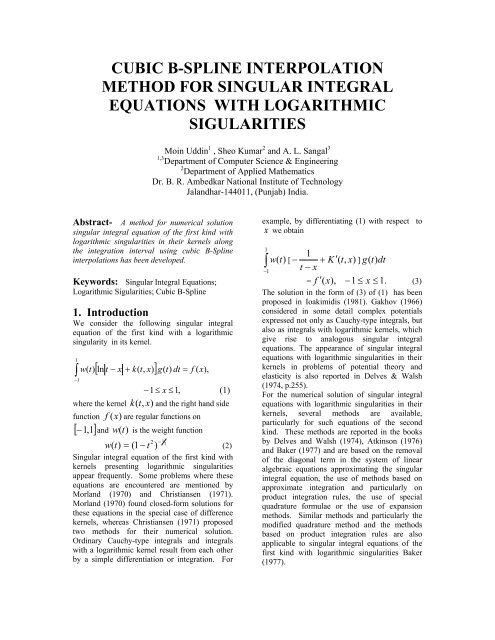
CUBIC B-SPLINE INTERPOLATION<br />
METHOD FOR SINGULAR INTEGRAL<br />
EQUATIONS WITH LOGARITHMIC<br />
SIGULARITIES<br />
Moin Uddin 1 , Sheo Kumar 2 and A. L. Sangal 3<br />
1,3 Department of Computer Science & Engineering<br />
2 Department of Applied Mathematics<br />
Dr. B. R. Ambedkar National Institute of Technology<br />
Jalandhar-144011, (Punjab) India.<br />
Abstract- A <strong>method</strong> <strong>for</strong> numerical solution<br />
<strong>singular</strong> <strong>integral</strong> equation of the first kind with<br />
logarithmic <strong>singular</strong>ities in their kernels along<br />
the integration interval using <strong>cubic</strong> B-Spline<br />
<strong>interpolation</strong>s has been developed.<br />
Keywords: Singular Integral Equations;<br />
Logarithmic Sigularities; Cubic B-Spline<br />
1. Introduction<br />
We consider the following <strong>singular</strong> <strong>integral</strong><br />
equation of the first kind with a logarithmic<br />
<strong>singular</strong>ity in its kernel.<br />
1<br />
∫<br />
−1<br />
w(<br />
t)<br />
[ ln t − x + k(<br />
t,<br />
x)<br />
]<br />
g(<br />
t)<br />
dt = f ( x),<br />
−1<br />
≤ x ≤1,<br />
(1)<br />
where the kernel k( t,<br />
x)<br />
and the right hand side<br />
function f (x)<br />
are regular functions on<br />
−1, 1 and w (t)<br />
is the weight function<br />
[ ]<br />
2 − 1<br />
2<br />
w ( t)<br />
= ( 1−<br />
t )<br />
(2)<br />
Singular <strong>integral</strong> equation of the first kind with<br />
kernels presenting logarithmic <strong>singular</strong>ities<br />
appear frequently. Some problems where these<br />
<strong>equations</strong> are encountered are mentioned by<br />
Morland (1970) and Christiansen (1971).<br />
Morland (1970) found closed-<strong>for</strong>m solutions <strong>for</strong><br />
these <strong>equations</strong> in the special case of difference<br />
kernels, whereas Christiansen (1971) proposed<br />
two <strong>method</strong>s <strong>for</strong> their numerical solution.<br />
Ordinary Cauchy-type <strong>integral</strong>s and <strong>integral</strong>s<br />
with a logarithmic kernel result from each other<br />
by a simple differentiation or integration. For<br />
example, by differentiating (1) with respect to<br />
x we obtain<br />
1<br />
∫<br />
−1<br />
1<br />
w (t)<br />
[ − + K ′ ( t,<br />
x)<br />
] g ( t)<br />
dt<br />
t − x<br />
= ′ ( x),<br />
−1<br />
≤ x ≤ 1.<br />
f (3)<br />
The solution in the <strong>for</strong>m of (3) of (1) has been<br />
proposed in Ioakimidis (1981). Gakhov (1966)<br />
considered in some detail complex potentials<br />
expressed not only as Cauchy-type <strong>integral</strong>s, but<br />
also as <strong>integral</strong>s with logarithmic kernels, which<br />
give rise to analogous <strong>singular</strong> <strong>integral</strong><br />
<strong>equations</strong>. The appearance of <strong>singular</strong> <strong>integral</strong><br />
<strong>equations</strong> with logarithmic <strong>singular</strong>ities in their<br />
kernels in problems of potential theory and<br />
elasticity is also reported in Delves & Walsh<br />
(1974, p.255).<br />
For the numerical solution of <strong>singular</strong> <strong>integral</strong><br />
<strong>equations</strong> with logarithmic <strong>singular</strong>ities in their<br />
kernels, several <strong>method</strong>s are available,<br />
particularly <strong>for</strong> such <strong>equations</strong> of the second<br />
kind. These <strong>method</strong>s are reported in the books<br />
by Delves and Walsh (1974), Atkinson (1976)<br />
and Baker (1977) and are based on the removal<br />
of the diagonal term in the system of linear<br />
algebraic <strong>equations</strong> approximating the <strong>singular</strong><br />
<strong>integral</strong> equation, the use of <strong>method</strong>s based on<br />
approximate integration and particularly on<br />
product integration rules, the use of special<br />
quadrature <strong>for</strong>mulae or the use of expansion<br />
<strong>method</strong>s. Similar <strong>method</strong>s and particularly the<br />
modified quadrature <strong>method</strong> and the <strong>method</strong>s<br />
based on product integration rules are also<br />
applicable to <strong>singular</strong> <strong>integral</strong> <strong>equations</strong> of the<br />
first kind with logarithmic <strong>singular</strong>ities Baker<br />
(1977).
The <strong>method</strong> described here uses Langrange<br />
<strong>interpolation</strong> on “practical” abscissas<br />
xk = cos( kπ<br />
/ n),<br />
k = 0(<br />
1)<br />
n.<br />
The related results are given below:<br />
Let Ln ( f ; x)<br />
denote the Lagrange polynomial<br />
of degree n interpolating f (x)<br />
at<br />
= kπ<br />
n k = We may write<br />
x k<br />
cos( / ), 0(<br />
1)<br />
n.<br />
n<br />
n<br />
∑ k<br />
k = 0<br />
L ( f ; x)<br />
= l ( x)<br />
f ( x ), (4)<br />
where the Langrange fundamental polynomials<br />
lk (x)<br />
are given by<br />
n<br />
lk ( x)<br />
( 2bk<br />
/ n)<br />
b jT<br />
j ( xk<br />
) T j ( x),<br />
= ∑<br />
j=<br />
0<br />
k<br />
k = 0(<br />
1)<br />
n,<br />
1 b =<br />
where 0 = n 2<br />
(5)<br />
b and<br />
bk = 1, k = 1(<br />
1)<br />
n −1.<br />
(x)<br />
T j are<br />
Chebyshev polynomials of the first kind. That<br />
lk ( x j ) = δ kj follows from the discrete<br />
orthogonality of the Chebyshev polynomials at<br />
the practical abscissas. For details, please see<br />
Chawla & Kumar (1979).<br />
For latest works on B-Spline, please see, Liu<br />
(1997), Prautzsch (2004) and Reif (2000).<br />
In past <strong>method</strong>s <strong>for</strong> solution of <strong>singular</strong> <strong>integral</strong><br />
<strong>equations</strong> with logarithmic <strong>singular</strong>ities have<br />
been also discussed in Alaylioglu & Lubinsky<br />
(1984), Atkinson & Sloan (1991), Atkinson<br />
(1988), Chakrabarti & Manam (2003), Saranen<br />
& Sloan (1992), Saranen (1991), Sloan & Burn<br />
(1992), Kress & Sloan (1993) and Manam<br />
(2003).<br />
2. The Numerical Method<br />
we consider the <strong>singular</strong> <strong>integral</strong> equation of the<br />
first kind with a logarithmic <strong>singular</strong>ity in its<br />
kernel.<br />
1<br />
∫<br />
−1<br />
w(<br />
t)<br />
[ ln t − x + k(<br />
t,<br />
x)<br />
]<br />
g(<br />
t)<br />
dt = f ( x),<br />
−1<br />
≤ x ≤ 1,<br />
where the kernel k( t,<br />
x)<br />
and the right hand side<br />
function f (x)<br />
are regular functions on<br />
−1, 1 and w(t) is the weight function<br />
[ ]<br />
2 − 1<br />
2<br />
w ( t)<br />
= ( 1−<br />
t )<br />
(7)<br />
In past a <strong>method</strong> <strong>for</strong> the <strong>integral</strong> equation (6)<br />
have been discussed in Ioakimidis (1981). In<br />
this chapter, we have described a <strong>cubic</strong> B-<strong>spline</strong><br />
approximation <strong>method</strong> <strong>for</strong> the numerical solution<br />
of (6), using uniqueness condition of the <strong>for</strong>m<br />
1<br />
∫<br />
−1<br />
w ( t)<br />
g(<br />
t)<br />
dt = C<br />
(8)<br />
where C is a known constant . Here, we have<br />
evaluated the <strong>integral</strong>s<br />
1<br />
( 4)<br />
( 4)<br />
L( Bn,<br />
j ; x)<br />
w(<br />
t)<br />
Bn,<br />
j ( t)<br />
ln t − x dt,<br />
= ∫<br />
−1<br />
m = 1(<br />
1)<br />
4,<br />
j = 1(<br />
1)<br />
n<br />
( 4)<br />
using the representation of Bn , j ( t)<br />
given<br />
below:<br />
(6)<br />
(9)
B<br />
( 4)<br />
n,<br />
j<br />
3<br />
⎧ ( t − t j )<br />
⎪<br />
,<br />
t j ≤ t ≤ t j+<br />
1,<br />
⎪(<br />
t j+<br />
3 − t j )( t j+<br />
1 − t j )( t j+<br />
2 − t j )<br />
⎪<br />
⎪ ( t − t j ) ⎡ ( t − t j )( t j+<br />
2 − t)<br />
( t j+<br />
3 − t)(<br />
t − t j+<br />
1)<br />
⎤<br />
⎪<br />
⎢<br />
+<br />
⎥<br />
( t j+<br />
3 − t j ) ⎢(<br />
2 )( 2 1)<br />
( 3 1)(<br />
2 1)<br />
⎪ ⎣ t j+<br />
− t j t j+<br />
− t j+<br />
t j+<br />
− t j+<br />
t j+<br />
− t j+<br />
⎥⎦<br />
⎪<br />
2<br />
(t j+<br />
4 − t)(<br />
t − t j+<br />
1)<br />
⎪ +<br />
, t j+<br />
1 ≤ t ≤ t j+<br />
2 ,<br />
⎪ ( t j+<br />
4 − t j+<br />
1)(<br />
t j+<br />
2 − t j+<br />
1)(<br />
t j+<br />
3 − t j+<br />
1)<br />
⎪<br />
⎪ ( t j+<br />
4 − t)<br />
⎡ ( t − t j+<br />
1)(<br />
t j+<br />
3 − t)<br />
( t j+<br />
4 − t)(<br />
t − t j+<br />
2 ) ⎤<br />
( t)<br />
= ⎨ ⎢<br />
+<br />
⎥<br />
⎪(<br />
t j+<br />
4 − t j+<br />
1)<br />
⎢⎣<br />
( t j+<br />
3 − t j+<br />
1)(<br />
t j+<br />
3 − t j+<br />
2 ) ( t j+<br />
4 − t j+<br />
2 )( t j+<br />
3 − t j+<br />
2 ) ⎥⎦<br />
⎪<br />
2<br />
⎪<br />
( t − t j )( t j+<br />
3 − t)<br />
+<br />
, t j+<br />
2 ≤ t ≤ t j+<br />
3,<br />
⎪ ( t j+<br />
3 − t j )( t j+<br />
3 − t j+<br />
1)(<br />
t j+<br />
3 − t j+<br />
2 )<br />
⎪<br />
3<br />
⎪ ( t j+<br />
4 − t)<br />
⎪<br />
,<br />
t j+<br />
3 ≤ t ≤ t j+<br />
4 ,<br />
⎪(<br />
t j+<br />
4 − t j+<br />
1)(<br />
t j+<br />
4 − t j+<br />
2 )( t j+<br />
4 − t j+<br />
3 )<br />
⎪<br />
0,<br />
otherwise.<br />
⎪<br />
⎪<br />
⎩<br />
(10)<br />
≤ t ≤ t ≤ t ≤ ⋅⋅<br />
⋅ ≤ t ≤ 1.<br />
Thus<br />
( 4)<br />
and replacing Bn , j ( t)<br />
by Lagrange<br />
<strong>interpolation</strong> at the “practical” abscissas<br />
xk = cos( kπ<br />
/ n),<br />
k = 0(<br />
1)<br />
n described in<br />
Chawla & Kumar (1979) and described here by<br />
<strong>equations</strong> (4) and (5). For derivation of (10),<br />
please see Prautzsch, Boehm & Paluszny [2002,<br />
pp. 61] & Phillips [2003, pp. 224]. The<br />
following results also have been used in the<br />
evaluation of <strong>singular</strong> <strong>integral</strong>s in (9):<br />
1<br />
∫ ( 0<br />
−1<br />
2 − 1<br />
2 1−<br />
t ) ln t − xT<br />
( t)<br />
dt = −π<br />
ln 2 , (11)<br />
− 1 0 1 2<br />
n+<br />
4<br />
( 4)<br />
{ Bn, j ( t)<br />
}<br />
{ } 4 n+<br />
( 4)<br />
t j and further B ( )<br />
j=<br />
0<br />
n,<br />
j t<br />
over interval ( j , t j+<br />
4 )<br />
is a <strong>cubic</strong> B-<strong>spline</strong> basis with knots<br />
is a <strong>cubic</strong> B-<strong>spline</strong><br />
t . Now, we have<br />
approximated unknown function g (t)<br />
as:<br />
n<br />
g ∑ j n,<br />
j<br />
j=<br />
0<br />
( 4)<br />
( t)<br />
≈ α B ( t)<br />
. (14)<br />
We get n <strong>equations</strong> from (6) using (14)<br />
n 1<br />
∑ ∫<br />
−<br />
[ ]<br />
α j w(<br />
t)<br />
ln t − xi<br />
( 4)<br />
+ k(<br />
t,<br />
xi<br />
) Bn,<br />
j ( t)<br />
dt<br />
1<br />
2 − 1<br />
π<br />
2<br />
∫ ( 1−<br />
t ) ln t − xT<br />
j ( t)<br />
dt = − T j ( x),<br />
j<br />
−1<br />
j=<br />
0<br />
j ≥ 1,<br />
(12)<br />
by<br />
1<br />
choosing<br />
= f ( xi<br />
),<br />
n collocation<br />
(15)<br />
points<br />
T j + 1(<br />
x)<br />
= 2xT<br />
j ( x)<br />
− T j−1<br />
( x);<br />
T0<br />
= 1,<br />
T1<br />
( x)<br />
= x.<br />
where T j (x)<br />
are Chebyshev polynomials of the<br />
first kind.<br />
(13) −1 < x 0 < x1<br />
< x2<br />
< ⋅⋅<br />
⋅ < xn−1<br />
< 1.<br />
Equation ( n + 1)<br />
th given below is obtained<br />
from <strong>equations</strong> (8) replacing g(t) by (14).<br />
Here, we have described a product integration<br />
<strong>method</strong> using <strong>cubic</strong> B-<strong>spline</strong> approximations <strong>for</strong><br />
unknown function g(t). Here, we have taken<br />
n + 5 knots<br />
n 1<br />
( 4)<br />
∑α j ∫ w( t)<br />
Bn,<br />
j ( t)<br />
dt = C . (16)<br />
j=<br />
0 −1
The values of α j , j = 0(<br />
1)<br />
n is obtained from<br />
the solution of above n + 1<strong>equations</strong><br />
using<br />
matrix inversion by partition <strong>method</strong>.<br />
3. Numerical Examples<br />
To illustrate the above <strong>method</strong> computationally,<br />
we consider the following two examples of<br />
<strong>singular</strong> <strong>integral</strong> <strong>equations</strong> with logarithmic<br />
<strong>singular</strong>ities:<br />
Example 1<br />
Consider the <strong>singular</strong> <strong>integral</strong> equation<br />
1<br />
2 − 1 ⎡<br />
1 ⎤<br />
2<br />
∫ ( 1−<br />
t ) ⎢ln<br />
t − x +<br />
( )<br />
( 10)<br />
⎥ g t dt<br />
1 ⎣ t + x +<br />
−<br />
⎦<br />
= f ( x),<br />
−1<br />
≤ x ≤ 1 (17)<br />
where the exact solution is given by<br />
t<br />
g ( t)<br />
= e<br />
and the values of f (x)<br />
have been computed.<br />
numerically at the various points of<br />
discretisations under the unique condition:<br />
1<br />
∫<br />
−1<br />
2 − 1<br />
2 ( 1−<br />
t ) g(<br />
t)<br />
dt = 2.<br />
493524565689<br />
.<br />
We solved the <strong>singular</strong> <strong>integral</strong> equation (17) by<br />
the present <strong>method</strong> <strong>for</strong> n = 20 and 40 <strong>for</strong> equally<br />
spaced mesh and choosing the collocation points<br />
sk = (tk + tk+1)/2, k = 0(1)n; we have solved linear<br />
algebraic system of <strong>equations</strong> using partition<br />
<strong>method</strong> <strong>for</strong> matrix inversion. The corresponding<br />
errors ek = | exact value (xk) − approximate<br />
value (xk) |<br />
<strong>for</strong> few points are listed in Table 1.<br />
Example 2<br />
Consider the <strong>singular</strong> <strong>integral</strong> equation<br />
1<br />
∫<br />
−1<br />
( 1−<br />
t<br />
2<br />
)<br />
−<br />
1<br />
2<br />
t+<br />
x<br />
[ ln t − x + e ]<br />
−1<br />
≤ x ≤ 1,<br />
g(<br />
t)<br />
dt = f ( x),<br />
where the exact solution is given by<br />
2 1<br />
2<br />
g( t)<br />
= ( 1−<br />
t )<br />
and the values of f (x)<br />
have been computed<br />
numerically at the various points of<br />
discretisations under the unique condition:<br />
1<br />
2 − 1<br />
2 ( 1−<br />
t ) g(<br />
t)<br />
dt = 2.<br />
00 .<br />
∫<br />
−1<br />
( 18)<br />
We solved the <strong>singular</strong> <strong>integral</strong> equation (18) by<br />
the present <strong>method</strong> <strong>for</strong> n = 20 and 40, <strong>for</strong> equally<br />
spaced mesh and choosing the collocation points<br />
sk = (tk + tk+1)/2, k = 0(1)n;<br />
We have solved linear algebraic system of<br />
<strong>equations</strong> using partition <strong>method</strong> <strong>for</strong> matrix<br />
inversion. The corresponding errors ek = |<br />
exact value (xk) − approximate value (xk) |<br />
<strong>for</strong> few points are listed in Table 2.<br />
Table 1<br />
Integral equation (17)<br />
n = 20 n = 40<br />
x h = 1/<br />
10 h = 1/<br />
20<br />
-1.00 9.16 E−05 1.52 E−06<br />
-.800 3.46 E−05 6.45 E−07<br />
-.600 3.29 E−05 2.99 E−06<br />
-.400 5.08 E−06 5.12 E−07.<br />
-.200 7.58 E−06 8.92 E−07<br />
0.00 6.13 E−05 5.56 E−07<br />
0.20 7.39 E−05 1.79 E−06<br />
0.40 8.15 E−06 8.54 E−07<br />
0.60 9.85 E−05 8.77 E−07<br />
0.80 1.36 E−05 5.37 E−06<br />
1.00 3.48 E−06 6.59 E−07<br />
Table 2<br />
Integral equation (18)<br />
n = 20 n = 40<br />
x h = 1/<br />
10 h = 1/<br />
20<br />
-1.00 1.16 E−03 4.78 E−04<br />
-.800 2.93 E−03 9.28 E−05<br />
-.600 4.72 E−03 8.54E−04<br />
-.400 6.09 E−04 1.19 E−05.<br />
-.200 7.27 E−04 2.12 E−05<br />
0.00 8.15 E−04 4.85 E−05<br />
0.20 9.46 E−04 6.81 E−04<br />
0.40 1.24 E−04 6.75 E−05<br />
0.60 2.54 E−04 4.93 E−06<br />
0.80 3.19 E−04 3..46 E−06<br />
1.00 8.45 E−04 8.49E−06
References<br />
[1] A. Alaylioglu and D. S. Lubinsky,<br />
“Product integration of logarithmic<br />
<strong>singular</strong> integrands based on <strong>cubic</strong><br />
<strong>spline</strong>”; Journal of Computational and<br />
Applied Mathematics 11, 353-366<br />
(1984).<br />
[2] K. E. Atkinson and I. H. Sloan, “The<br />
numerical solution of first kind<br />
logarithmic-kernal <strong>integral</strong> <strong>equations</strong><br />
on smooth open arcs” ; Math.<br />
Comput., 56, 119-139, (1991).<br />
[3] K. E. Atkinson, “A Survey of<br />
Numerical Methods <strong>for</strong> the Solution of<br />
Fredholm Integral Equations of the<br />
second kind”; Society <strong>for</strong> Industrial<br />
and Applied Mathematics (SIAM),<br />
Philadelphia, Pensylvania, 1976.<br />
[4] K. E. Atkinson, “A discrete Galerkin<br />
<strong>method</strong> <strong>for</strong> first kind <strong>integral</strong> <strong>equations</strong><br />
with logarithmic kernel”; J. Integral<br />
Eqns. Applics. 1, 343-363, (1988).<br />
[5] C. T. H. Baker, “The Numerical<br />
Treatment of Integral Equations”;<br />
Clarendon Press, 1977.<br />
[6] A. Chakrabarti, and S. R. Manam,<br />
“Solution of a logarithmic <strong>singular</strong><br />
<strong>integral</strong> equation”; Applied<br />
Mathematics Letters, 16, 369-373,<br />
(2003).<br />
[7] M. M. Chawla , and S. Kumar,<br />
“Convergence of quadratures <strong>for</strong><br />
Cauchy principal value <strong>integral</strong>s”;<br />
Computing, 23, 67-72, (1979).<br />
[8] S. Christiansen , “Numerical solution<br />
of an <strong>integral</strong> <strong>equations</strong> with a<br />
logarithmic kernel”; BIT, 11, 276-<br />
287, (1971).<br />
[9] L.M. Delves, and J. Walsh, (Eds),<br />
“Numerical Solution of Integral<br />
Equations”; Ox<strong>for</strong>d University Press,<br />
London, 1974.<br />
[10] F. D. Gakhov, “Boundary value<br />
problems”; Pergamen Press and<br />
Addison- Wesley, Ox<strong>for</strong>d, 1966.<br />
[11] N. I. Ioakimidis, “A <strong>method</strong> <strong>for</strong><br />
numerical solution of <strong>singular</strong> <strong>integral</strong><br />
<strong>equations</strong> with logarithm<br />
<strong>singular</strong>ities”; Iternational J.<br />
Computer Math., 9, 363-372, (1981).<br />
[12] R. Kress, and I. H. Sloan, “On the<br />
numerical solution of a logarithmic<br />
<strong>integral</strong> equation of the first kind <strong>for</strong><br />
the Helmholtz equation”; Numer.<br />
Math., 66, 199-214, (1993).<br />
[13] W. Liu, “A simple, efficient degree<br />
raising algorithm <strong>for</strong> B-Spline curves”;<br />
Computer Aided Geometric Design,<br />
14, 693-698, (1997).<br />
[14] S. R. Manam, “A logarithmic <strong>singular</strong><br />
<strong>integral</strong> equation over multiple<br />
intervals”; Applied Mathematics<br />
Letters, 16, 1031-1037, (2003).<br />
[15] L. W. Morland, “Singular <strong>integral</strong><br />
<strong>equations</strong> with logarithmic kernels”;<br />
Mathematika, 17, (1970), 47−56,<br />
(1970).<br />
[16] G. M. Phillips, “Interpolations and<br />
Approximations by Polynomials”;<br />
Springer-Verlag, New York, 2003.<br />
[17] H. Prautzsch, W. Boehm, and M.<br />
Paluszny, “Bézier and B-<strong>spline</strong><br />
Techniques”; Springer-Verlag, Berlin,<br />
2002.<br />
[18] H. Prautzsch, “B-<strong>spline</strong>s with arbitrary<br />
connection matrices”; Constructive<br />
Approximation, 20, 191-205, (2004).<br />
[19] U. Reif, “Best bounds on the<br />
approximation of polynomials and<br />
<strong>spline</strong>s by their control structure”;<br />
Computer Aided Geometric Design,<br />
17, 579-589, (2000).<br />
[20] J. Saranen, and I. H. Sloan,<br />
“Quadrature <strong>method</strong>s <strong>for</strong> logarithmic-<br />
kernel <strong>integral</strong> <strong>equations</strong> on closed<br />
curves”; IMA Journal of Numerical<br />
Analysis, 12, 167- 187, (1992).<br />
[21] J. Saranen, “The modified quadrature<br />
<strong>method</strong> <strong>for</strong> logarithmic-kernel <strong>integral</strong><br />
<strong>equations</strong> on closed curves”; J.<br />
Integral Equations Appl., 3, 575-600<br />
(1991).<br />
[22] I. H. Sloan, and B. J. Burn, “An<br />
unconventional quadrature <strong>method</strong> <strong>for</strong><br />
logarithmic-kernel <strong>integral</strong> <strong>equations</strong><br />
of closed curves”; J. Integral<br />
Equations Appl., 4, 117-151 (1992).