cubic b-spline interpolation method for singular integral equations ...
cubic b-spline interpolation method for singular integral equations ...
cubic b-spline interpolation method for singular integral equations ...

You also want an ePaper? Increase the reach of your titles
YUMPU automatically turns print PDFs into web optimized ePapers that Google loves.
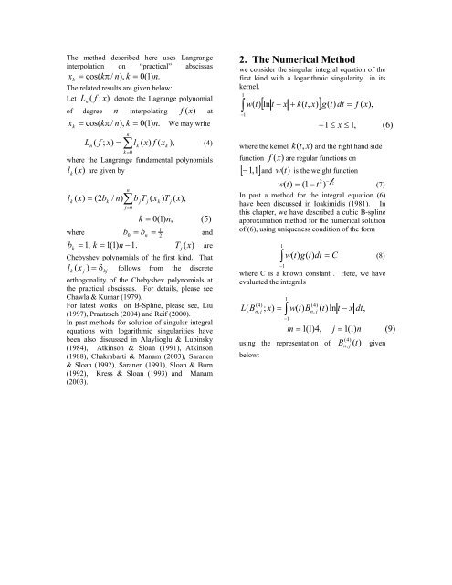
The <strong>method</strong> described here uses Langrange<br />
<strong>interpolation</strong> on “practical” abscissas<br />
xk = cos( kπ<br />
/ n),<br />
k = 0(<br />
1)<br />
n.<br />
The related results are given below:<br />
Let Ln ( f ; x)<br />
denote the Lagrange polynomial<br />
of degree n interpolating f (x)<br />
at<br />
= kπ<br />
n k = We may write<br />
x k<br />
cos( / ), 0(<br />
1)<br />
n.<br />
n<br />
n<br />
∑ k<br />
k = 0<br />
L ( f ; x)<br />
= l ( x)<br />
f ( x ), (4)<br />
where the Langrange fundamental polynomials<br />
lk (x)<br />
are given by<br />
n<br />
lk ( x)<br />
( 2bk<br />
/ n)<br />
b jT<br />
j ( xk<br />
) T j ( x),<br />
= ∑<br />
j=<br />
0<br />
k<br />
k = 0(<br />
1)<br />
n,<br />
1 b =<br />
where 0 = n 2<br />
(5)<br />
b and<br />
bk = 1, k = 1(<br />
1)<br />
n −1.<br />
(x)<br />
T j are<br />
Chebyshev polynomials of the first kind. That<br />
lk ( x j ) = δ kj follows from the discrete<br />
orthogonality of the Chebyshev polynomials at<br />
the practical abscissas. For details, please see<br />
Chawla & Kumar (1979).<br />
For latest works on B-Spline, please see, Liu<br />
(1997), Prautzsch (2004) and Reif (2000).<br />
In past <strong>method</strong>s <strong>for</strong> solution of <strong>singular</strong> <strong>integral</strong><br />
<strong>equations</strong> with logarithmic <strong>singular</strong>ities have<br />
been also discussed in Alaylioglu & Lubinsky<br />
(1984), Atkinson & Sloan (1991), Atkinson<br />
(1988), Chakrabarti & Manam (2003), Saranen<br />
& Sloan (1992), Saranen (1991), Sloan & Burn<br />
(1992), Kress & Sloan (1993) and Manam<br />
(2003).<br />
2. The Numerical Method<br />
we consider the <strong>singular</strong> <strong>integral</strong> equation of the<br />
first kind with a logarithmic <strong>singular</strong>ity in its<br />
kernel.<br />
1<br />
∫<br />
−1<br />
w(<br />
t)<br />
[ ln t − x + k(<br />
t,<br />
x)<br />
]<br />
g(<br />
t)<br />
dt = f ( x),<br />
−1<br />
≤ x ≤ 1,<br />
where the kernel k( t,<br />
x)<br />
and the right hand side<br />
function f (x)<br />
are regular functions on<br />
−1, 1 and w(t) is the weight function<br />
[ ]<br />
2 − 1<br />
2<br />
w ( t)<br />
= ( 1−<br />
t )<br />
(7)<br />
In past a <strong>method</strong> <strong>for</strong> the <strong>integral</strong> equation (6)<br />
have been discussed in Ioakimidis (1981). In<br />
this chapter, we have described a <strong>cubic</strong> B-<strong>spline</strong><br />
approximation <strong>method</strong> <strong>for</strong> the numerical solution<br />
of (6), using uniqueness condition of the <strong>for</strong>m<br />
1<br />
∫<br />
−1<br />
w ( t)<br />
g(<br />
t)<br />
dt = C<br />
(8)<br />
where C is a known constant . Here, we have<br />
evaluated the <strong>integral</strong>s<br />
1<br />
( 4)<br />
( 4)<br />
L( Bn,<br />
j ; x)<br />
w(<br />
t)<br />
Bn,<br />
j ( t)<br />
ln t − x dt,<br />
= ∫<br />
−1<br />
m = 1(<br />
1)<br />
4,<br />
j = 1(<br />
1)<br />
n<br />
( 4)<br />
using the representation of Bn , j ( t)<br />
given<br />
below:<br />
(6)<br />
(9)