LQR control for a rotary double inverted pendulum - Nguyen Dang ...
LQR control for a rotary double inverted pendulum - Nguyen Dang ...
LQR control for a rotary double inverted pendulum - Nguyen Dang ...

Create successful ePaper yourself
Turn your PDF publications into a flip-book with our unique Google optimized e-Paper software.
<strong>LQR</strong> <strong>control</strong> <strong>for</strong> a <strong>rotary</strong> <strong>inverted</strong> <strong>pendulum</strong><br />
C. Mira 1<br />
1 Program of Physical Engineering, School of Science and Humanities, EAFIT University, Medellín, Colombia<br />
Abstract - This paper presents the procedure to obtain a<br />
Linear Quadratic Regulator (<strong>LQR</strong>) <strong>control</strong> <strong>for</strong> a <strong>rotary</strong><br />
<strong>double</strong> <strong>inverted</strong> <strong>pendulum</strong>. The theoretical description of<br />
the movement is developed using the Euler-Lagrange<br />
equations and it is implemented using Maple. Analysis of<br />
stability, <strong>control</strong>lability and observability are carried<br />
out, also, using Maple tools. Finally the obtained <strong>control</strong><br />
is presented as a linear combination of the dynamic<br />
variables of the system. Also is shown the evolution of<br />
these variables from a set of initial conditions to a stable<br />
state and is exposed a short analysis about the ability of<br />
response of the <strong>control</strong> respect the initial conditions.<br />
Keywords: Rotary <strong>double</strong> <strong>inverted</strong> <strong>pendulum</strong>, <strong>control</strong><br />
<strong>LQR</strong>, Euler-Lagrange.<br />
1 Introduction<br />
The <strong>inverted</strong> <strong>pendulum</strong> is a typical nonlinear<br />
mechanical system used <strong>for</strong> testing <strong>control</strong> algorithms<br />
[1]. Generally, these <strong>control</strong> system are based in<br />
feedback <strong>control</strong> methods. They are different kinds of<br />
<strong>inverted</strong> <strong>pendulum</strong>, but the common goal is to balance a<br />
link on end using feedback <strong>control</strong> [2].<br />
In this paper the case of study is a multiple input<br />
single output <strong>control</strong> <strong>for</strong> a <strong>rotary</strong> <strong>double</strong> <strong>inverted</strong><br />
<strong>pendulum</strong>. The rotational is a rather challenging<br />
<strong>inverted</strong> <strong>pendulum</strong> [2].<br />
2 Problem<br />
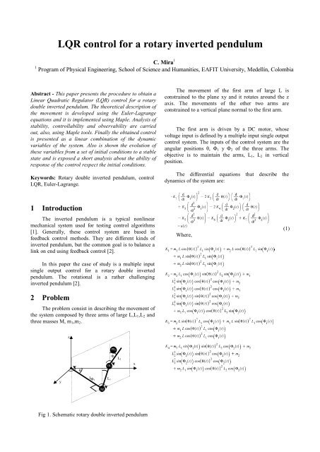
The problem consist in describing the movement of<br />
the system composed by three arms of large L,L1,L2 and<br />
three masses M, m1,m2.<br />
y<br />
z<br />
θ<br />
L<br />
Ф1<br />
Fig 1. Schematic <strong>rotary</strong> <strong>double</strong> <strong>inverted</strong> <strong>pendulum</strong><br />
M<br />
m1<br />
L1<br />
m2<br />
Ф<br />
2<br />
L2<br />
x<br />
The movement of the first arm of large L is<br />
constrained to the plane xy and it rotates around the z<br />
axis. The movements of the other two arms are<br />
constrained to a vertical plane normal to the first arm.<br />
The first arm is driven by a DC motor, whose<br />
voltage input is defined by a multiple input single output<br />
<strong>control</strong> system. The inputs of the <strong>control</strong> system are the<br />
angular positions θ, Φ1 y Φ2 of the three arms. The<br />
objective is to maintain the arms, L1, L2 in vertical<br />
position.<br />
The differential equations that describe the<br />
dynamics of the system are:<br />
Where,<br />
(1)
In this expression u(t) is the output of the <strong>control</strong><br />
system.<br />
Where,<br />
Where,<br />
(2)<br />
(3)<br />
3 Method<br />
The equations that describe the problem are<br />
developed using Euler-Lagrange mechanics. The<br />
lagrangian is the difference between the kinetic energy<br />
and the potential energy. For the system under study it<br />
could be written as:<br />
Where,<br />
The equations of motion are obtained by means of<br />
the minimum action principle. Where the action is<br />
defined as:<br />
Functional derivatives of the action respect each<br />
movement parameter (θ, Ф1, Ф2) are computed. The<br />
functional derivative of the action respect the angle θ is<br />
equal to u(t), which is the only external action in the<br />
system. The functional derivatives of the action respect<br />
Ф1 and Ф2 are equal to zero.<br />
Subsequently the movement equations are solved<br />
<strong>for</strong> the angular velocities. Controllability and<br />
observability matrices are constructed to verify that the<br />
(4)<br />
(5)
system with particular parameter values (M, m1, m2, L,<br />
L1, and L2) is <strong>control</strong>lable. Finally the <strong>LQR</strong> <strong>control</strong> is<br />
computed and simulations of it behaviour are made.<br />
4 Results<br />
A <strong>control</strong>led is designed <strong>for</strong> a system with the<br />
parameters listed in the table 1.<br />
Table 1 Parameters values<br />
Parameter Value<br />
g 9.8 m/s 2<br />
M 10 kg<br />
m1 2 kg<br />
m2 1.5 kg<br />
L 3 m<br />
L1<br />
1 m<br />
0.5 m<br />
L2<br />
The <strong>LQR</strong> <strong>control</strong>ler is founded as a linear<br />
combination of the dynamic variables of the system.<br />
For implementation purposes the output of the<br />
<strong>control</strong> is converted in a voltage signal. The input<br />
variables are sensed by linear potentiometers and are<br />
analogical differentiated. A summation of the input<br />
variables regulated by resistances, proportional to the<br />
coefficients in the linear combination, is made to obtain<br />
the output voltage. A scheme of the analogical <strong>control</strong><br />
system is shown in the figure 2.<br />
Fig 2. Analogical circuit <strong>for</strong> the <strong>control</strong> system<br />
Also simulations of the behaviour of the <strong>control</strong> are<br />
made. By means of these simulations is found that the<br />
initial values of the angles Ф1 and Ф2 are limited to a<br />
maximum value 36 degrees.<br />
(6)<br />
In the following graphics some results are shown<br />
<strong>for</strong> a particular case of solution where the initial<br />
conditions were those listed in the table 2.<br />
Table 2 Initial conditions <strong>for</strong> a particular case of study<br />
Value<br />
Angle<br />
(degrees)<br />
θ 0<br />
Ф1 18<br />
32.7<br />
Ф2<br />
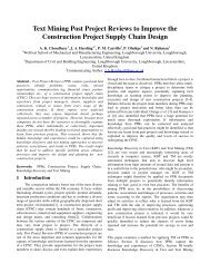
The evolution of position of the arm <strong>control</strong> driven<br />
from the initial condition to the equilibrium condition is<br />
shown in the figure 3.<br />
Fig 3 Evolution of θ <strong>for</strong> the particular case of study<br />
(angle in radians, time in seconds).<br />
The evolutions of the angular positions of the<br />
<strong>inverted</strong> arms are shown in figures 4 and 5.<br />
Fig 4 Evolution of Ф1 <strong>for</strong> the particular case of study<br />
(angle in radians, time in seconds).
Fig 5 Evolution of Ф2 <strong>for</strong> the particular case of study<br />
(angle in radians, time in seconds).<br />
5 Conclusions<br />
A <strong>LQR</strong> <strong>control</strong> <strong>for</strong> a <strong>double</strong> <strong>inverted</strong> <strong>pendulum</strong> was<br />
developed. This <strong>control</strong> is represented by a linear<br />
combination of the dynamic variables of the system, then<br />
is feasible its implementation with analogical<br />
electronics.<br />
Animations made show that the angles that<br />
describe the positions of the elements evolve to<br />
equilibrium conditions.<br />
The <strong>control</strong> found has a lower robustness because it<br />
only allows initial angles lower than 36 degrees. A more<br />
robust <strong>control</strong> system would imply more advanced<br />
techniques.<br />
The use of advanced computation tools like Maple<br />
has great advantages. Otherwise long mathematic<br />
operations should be made involving a lot of time and<br />
limiting the possibility of changing parameters.<br />
The <strong>for</strong>mulation of Euler-Lagrange mechanics<br />
allows finding the movement equations of the system in<br />
consistent way. These procedure is also facilitate by the<br />
use ·Physics Maple library.<br />
6 References<br />
[1] S.A: Reshmin and F. L. Chernous’ko. “A Time-<br />
Optimal Control Synthesis <strong>for</strong> a Nonlinear Pendulum”.<br />
Journal of Computer and Systems Sciences<br />
International, 2007, Vol. 46, No. 1, pp. 9–18. ISSN<br />
1064-2307.<br />
[2] S. Awtar, N. King, T. Allen, I. Bang, M. Hagan,<br />
D. Skidmore, K. Craig. “Inverted Pendulum Systems:<br />
Rotary and Arm-Driven: A Mechatronic System Design<br />
Case Study”. Mechatronics. Department of Mechanical<br />
Engineering, Aeronautical Engineering and Mechanics<br />
Rensselaer Polytechnic Institute<br />
[3] K. D. Pham, M. K. Sain, and S. R. LIBERTY<br />
“Cost Cumulant Control: State-Feedback, Finite-<br />
Horizon Paradigm with Application to Seismic<br />
Protection”. Journal of Optimization Theory and<br />
Applications: Vol. 115, No. 3, pp. 685–710, December<br />
2002.