Numerical analysis of time discretization of optimal control problems
Numerical analysis of time discretization of optimal control problems
Numerical analysis of time discretization of optimal control problems

You also want an ePaper? Increase the reach of your titles
YUMPU automatically turns print PDFs into web optimized ePapers that Google loves.
<strong>Numerical</strong> <strong>analysis</strong> <strong>of</strong> <strong>time</strong> <strong>discretization</strong> <strong>of</strong><br />
<strong>optimal</strong> <strong>control</strong> <strong>problems</strong><br />
J. Frédéric Bonnans<br />
INRIA Saclay and CMAP, Ecole Polytechnique<br />
Applied and <strong>Numerical</strong> Optimal Control<br />
ITN-SADCO, 23-27 April 2012, Paris
I: ORIENTATION<br />
We consider the problem <strong>of</strong> minimizing the cost function<br />
T<br />
0<br />
as well as<br />
ℓ(ut,yt)dt+φ(y0,yT) subject to: ˙yt = f(ut,yt), t ∈ (0,T),<br />
Control constraints: c(ut) ≤ 0, t ∈ (0,T)<br />
State constraints: g(yt) ≤ 0, t ∈ (0,T)<br />
Mixed state and <strong>control</strong> constraints: c(ut,yt) ≤ 0, t ∈ (0,T)<br />
Initial-final equality and inequality constraints:<br />
Φi(y0,yT) = 0, i = 1,...,r1,<br />
Φi(y0,yT) ≤ 0, i = r1+1,...,r.<br />
1
This class <strong>of</strong> <strong>problems</strong> is quite large:<br />
• It includes the case <strong>of</strong> design parameters = states with zero derivative<br />
Special case: variable horizon ˙yt = Tf(ut,yt), t ∈ (0,1)<br />
• If data depend smoothly on <strong>time</strong>, we may set <strong>time</strong> as a state with<br />
derivative equal to 1<br />
• Multiphases systems (separation <strong>of</strong> stage rockets) enter in this<br />
framework by setting “phases in parallel”<br />
• We may skip the integral cost, adding ˙yn+1 = ℓ(ut,yt).<br />
The new cost is yn+1,T +φ(y0,yT)<br />
• It includes some delay systems (H. Maurer)<br />
2
Function spaces<br />
• Control and state spaces<br />
U := L ∞ (0,T;R m ); Y := W 1,∞ (0,T;R n ).<br />
Their extension to Hilbert spaces<br />
U2 := L 2 (0,T;R m ); Y2 := H 1 (0,T;R n ).<br />
3
The Euler <strong>discretization</strong><br />
• N: number <strong>of</strong> <strong>time</strong> steps, hk > 0 duration <strong>of</strong> kth <strong>time</strong> step<br />
• Steps begin/end at <strong>time</strong> t0 = 0, and for k = 1 to N, tk = k<br />
j=0 hk<br />
• State equation: yk+1 = yk +hkf(uk,yk), k = 0,...,N −1.<br />
• Cost function: φ(yN)<br />
Running constraints:<br />
c(uk) ≤ 0; g(yk) ≤ 0; c(uk,yk) ≤ 0, k = 1,...,N −1<br />
Final equality and inequality constraints:<br />
Φi(y0,yN) = 0, i = 1,...,r1,<br />
Φi(y0,yN) ≤ 0, i = r1+1,...,r.<br />
4
Basic questions on the numerical <strong>analysis</strong><br />
Given a nominal local solution (ū,¯y) <strong>of</strong> the original problem:<br />
• Has the discretized problem a solution (u h ,y h ) near (ū,¯y) ??<br />
• Error order u h −ū+y h − ¯y = O( ¯ h), where ¯ h := maxkhk ?<br />
• Design <strong>of</strong> higher-order schemes ?<br />
• Assumptions <strong>of</strong> (piecewise) smooth solutions: it is true ?<br />
• How do we solve the discretized problem ?<br />
5
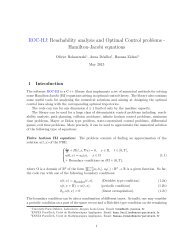
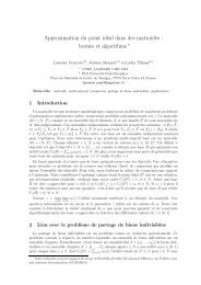
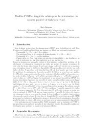
The simplest <strong>optimal</strong> <strong>time</strong> problem I<br />
Reach the zero state: dynamics ¨xt = ut ∈ [−1,1].<br />
0.5<br />
0.4<br />
0.3<br />
0.2<br />
0.1<br />
-0.1<br />
-0.2<br />
-0.3<br />
-0.4<br />
-0.5<br />
0<br />
-0.16 -0.12 -0.08 -0.04 0 0.04 0.08 0.12 0.16<br />
Figure 1: Control synthesis: state space<br />
6
The simplest <strong>optimal</strong> <strong>time</strong> problem II<br />
• Solution: Bang-bang <strong>optimal</strong> <strong>control</strong>, at most one switching <strong>time</strong><br />
• Discretized solution <strong>of</strong> same nature (costate affine function <strong>of</strong> <strong>time</strong>)<br />
• Exact integrators <strong>control</strong> constant over a <strong>time</strong>: mid point rule<br />
• In that case, error only due to the switching <strong>time</strong> step<br />
• Expected error: at most O( ˜ h), with ˜ h = <strong>time</strong> step a switching <strong>time</strong>.<br />
Ref. for LQ bang-bang <strong>problems</strong> Alt, Baier, Gerdts, Lempio, Error<br />
bounds for Euler approximation <strong>of</strong> linear-quadratic <strong>control</strong> <strong>problems</strong> with<br />
bang-bang solutions. Preprint, 2010.<br />
7
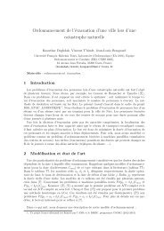
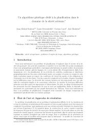
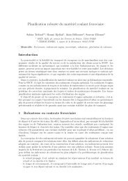
Fuller’s problem I (work with J. Laurent-Varin)<br />
Same dynamics: ¨xt = ut ∈ [−1,1]; Integral cost T<br />
0 x2 tdt.<br />
1.0<br />
0.8<br />
0.6<br />
0.4<br />
0.2<br />
0.0<br />
−0.2<br />
−0.4<br />
−0.6<br />
−0.8<br />
−1.0<br />
0 1 2 3 4 5 6 7 8<br />
Figure 2: Fuller problem: <strong>optimal</strong> <strong>control</strong>, logarithmic penalty<br />
8
Fuller’s problem II<br />
• Known true solution (Fuller 1963)<br />
• Sequence <strong>of</strong> bang-bang arcs whose length geometrically converges to 0<br />
• Followed by singular arc: u = 0 and x = 0.<br />
• Again we can use “exact” integrators for a <strong>control</strong> constant over <strong>time</strong><br />
steps<br />
• Averaging effect: loss <strong>of</strong> <strong>optimal</strong>ity maybe smaller than it seems.<br />
9
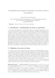
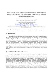
Robbins state constrained problem I<br />
• Dynamics: ¨x (3)<br />
t = ut ∈ [−1,1];<br />
• cost T<br />
0 (xt+u 2 t)dt, constraint x ≥ 0.<br />
• Optimal state: infinitely many isolated touch points converging to the<br />
entry point <strong>of</strong> a boundary arc x = 0.<br />
• Optimal <strong>control</strong>: infinitely many damped oscillations followed by an arc<br />
with zero values <strong>of</strong> the <strong>control</strong><br />
10
Robbins state constrained problem II<br />
1.0<br />
0.9<br />
0.8<br />
0.7<br />
0.6<br />
0.5<br />
0.4<br />
0.3<br />
0.2<br />
0.1<br />
0.0<br />
0 1 2 3 4 5 6 7<br />
Figure 3: Robbins problem: exact solution, plot in A. Hermant PhD thesis<br />
11
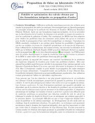
Robbins state constrained problem III<br />
Figure 4: Robbins problem: Bocop output <strong>of</strong> the <strong>control</strong><br />
12
Robbins state constrained problem IV<br />
0.03<br />
0.02<br />
0.01<br />
0<br />
-0.01<br />
-0.02<br />
-0.03<br />
-0.04<br />
-0.05<br />
Mesh Reffinement on a given interval<br />
N=200<br />
N=200 + 1000 on [4;6]<br />
4.6 4.8 5 5.2 5.4 5.6 5.8 6<br />
Figure 5: Robbins problem: Refinement <strong>of</strong> grid <strong>discretization</strong><br />
13
Beam problem: a second-order state constraint<br />
0.28<br />
0.24<br />
0.20<br />
0.16<br />
0.12<br />
0.08<br />
0.04<br />
0<br />
0 0.1 0.2 0.3 0.4 0.5 0.6 0.7 0.8 0.9 1.0<br />
Figure 6: Beam problem<br />
Dynamics ¨xt = ut ∈ [−1,1]. Cost 1<br />
0 u2 tdt; constraint x ≤ xMAX.<br />
Drawing: <strong>optimal</strong> displacement function <strong>of</strong> xMAX.<br />
14
II: UNCONSTRAINED PROBLEMS: minimize the cost function<br />
T<br />
ℓ(ut,yt)dt+φ(y0,yT)<br />
subject to<br />
0<br />
˙yt = f(ut,yt), t ∈ (0,T); y0 = y 0 .<br />
Optimality conditions: Costate equation along the trajectory (ū,¯y):<br />
−˙¯pt = ¯ptfy(ūt,¯yt), t ∈ (0,T); ¯pT = φ ′ (¯yT).<br />
Pontryagin’s principle (PMP): H[p](u,y) := pf(u,y)<br />
and in particular<br />
H[¯pt](ūt,¯yt) ≤ H[¯pt](u,¯yt), for all u ∈ R m , for a.a. t<br />
Hu[¯pt](ūt,¯yt) = 0, t ∈ (0,T).<br />
15
Discretization by Euler’s method<br />
⎧<br />
⎨<br />
⎩<br />
Min φ(yN);<br />
yk+1 = yk +hkf(uk,yk), k = 0,...,N −1,<br />
y0 = y 0 .<br />
hk > 0: kth step size; the discretized <strong>time</strong>s: t0 = 0,<br />
Lagrangian:<br />
tk :=<br />
φ(yN)+p0(y 0 −y0)+<br />
k−1 <br />
i=0<br />
(1)<br />
hi, k = 1,...,N. (2)<br />
N−1 <br />
k=0<br />
pk+1(yk +hkf(uk,yk)−yk+1).<br />
16
Optimality systems (original and discretized problem)<br />
For the original problem:<br />
⎧<br />
⎪⎨<br />
⎪⎩<br />
˙yt = f(ut,yt),<br />
−˙¯pt = pfy(ut,yt), t ∈ (0,T);<br />
0 = pfu(ut,yt), t ∈ (0,T);<br />
y0 = y 0 ; pT = φ ′ (¯yT),<br />
and for the discretized problem<br />
⎧<br />
yk+1−yk<br />
⎪⎨<br />
hk<br />
pk −pk+1<br />
= f(uk,yk),<br />
= pk+1fy(uk,yk), k = 0,...,N −1,<br />
⎪⎩<br />
hk<br />
0 = pk+1fu(uk,yk), k = 0,...,N −1,<br />
y0 = y 0 ; pN = φ ′ (yN).<br />
17
Reduction by elimination <strong>of</strong> the <strong>control</strong>: continuous problem<br />
Reduction hypothesis: ū continous, and<br />
Huu[¯pt](ūt,¯yt) = ¯ptfuu(ūt,¯yt) uniformly invertible.<br />
Then by the IFT (Implicit function theorem), “locally in <strong>time</strong>”<br />
Reduced <strong>optimal</strong>ity system:<br />
⎧<br />
⎨<br />
⎩<br />
Hu[p](u,y) = 0 iff u = Υ(p,y).<br />
˙yt = f(Υ(yt,pt),yt),<br />
−˙¯pt = pfy(Υ(yt,pt),yt), t ∈ (0,T);<br />
y0 = y 0 ; pT = φ ′ (¯yT),<br />
18
Shooting problem: continuous problem<br />
• Let p[p0], y[p0] denote the solution <strong>of</strong> the previous ODE with initial<br />
condition (y 0 ,p0).<br />
• Shooting function: S(p0) = pT[p0]−φ ′ (yT[p0]).<br />
• Optimality system ⇔ Shooting equation: S(p0) = 0.<br />
• Assume ¯p0 well-posed solution: S(¯p0) = 0, and S ′ (¯p0) invertible.<br />
• Then locally: ¯p0 unique solution, Newton’s method converges, and<br />
sensitivity <strong>analysis</strong> thanks to IFT.<br />
19
Shooting problem: discretized problem<br />
• Reduced formulation by elimination <strong>of</strong> the <strong>control</strong>:<br />
⎧<br />
⎪⎨<br />
⎪⎩<br />
yk+1−yk<br />
hk<br />
pk −pk+1<br />
hk<br />
= f(Υ(yk,pk),yk),<br />
= pk+1fy(Υ(yk,pk),yk), k = 0,...,N −1,<br />
y0 = y 0 ; pN = φ ′ (yN).<br />
• Let p h [p0], y h [p0] denote the solution <strong>of</strong> the previous ODE with initial<br />
condition (y 0 ,p0) (well-defined if p0 close to ¯p0 and ¯ h small)<br />
• Optimality system ⇔ S h (p0) := p h T [p0]−φ ′ (y h T [p0]) = 0.<br />
20
Partitioned Euler integrators<br />
• Consider the partitioned ODE<br />
˙y = F(y,p); ˙p = G(y,p)<br />
• Associated partitioned Euler scheme:<br />
yk+1−yk<br />
hk<br />
= F(yk,pk+1);<br />
pk+1−pk<br />
hk<br />
= G(yk,pk+1);<br />
• Here: F(y,p) = f(Υ(y,p),y); G(y,p) = −pfy(Υ(y,p),y).<br />
• It can easily be checked that<br />
S h → S locally uniformly as well as its derivatives.<br />
21
Error <strong>analysis</strong><br />
• F: set <strong>of</strong> C 1 mappings R n → R n in ¯ B(¯p0,1).<br />
• Define Ξ : R n ×F → R n , (p0,F) ↦→ Ξ(p0,F) := F(p0).<br />
• Clearly Ξ is C 1 and ∂Ξ(p0,F)<br />
∂p0<br />
= F ′ (p0).<br />
• If invertible, we can apply the IFT (Banach space setting) to Ξ at (¯p0,S).<br />
• Conclusion: there exists a locally unique ¯p h 0 solution <strong>of</strong> S h (¯p h 0) = 0<br />
• Error estimate: |¯p h 0 − ¯p0| = O(S h −S) = O( ¯ h).<br />
More precisely: |¯p h 0 − ¯p0| = O(S h (¯p0)|).<br />
22
What did we get ?<br />
• We deduce a uniform error estimate<br />
|ūt k −u h k|+|¯yt k −y h k|+|¯pt k −k h k| = O( ¯ h).<br />
• Thanks to the shooting approach, the <strong>analysis</strong> becomes trivial.<br />
• Link to second-order conditions ?<br />
• Higher-order methods ?<br />
23
Second-order <strong>optimal</strong>ity conditions<br />
• Cost function <strong>of</strong> <strong>control</strong>: J(u) := φ(yT[u]); class C ∞ : U → R.<br />
• Second-order necessary <strong>optimal</strong>ity condition: J ′′ (ū) 0.<br />
• Continuous extension <strong>of</strong> the quadratic form J ′′ (ū) to U2.<br />
• Second-order sufficient <strong>optimal</strong>ity condition SOSC: for some α > 0<br />
J ′′ (ū)(v,v) ≥ αv 2 2, for all v ∈ U2.<br />
• It characterizes quadratic growth: for some ε > 0 and any α ′ < α,<br />
J(ū+v) ≥ J(ū)+ 1<br />
2 α′ v 2 2, if v∞ ≤ ε.<br />
24
Computation <strong>of</strong> J ′′ (ū)<br />
• linearized state equation<br />
˙zt = Df(ūt,¯yt)(vt,zt), t ∈ (0,T), z0 = 0.<br />
• Hessian <strong>of</strong> Lagrangian, quadratic form over U, where z = z[v]:<br />
Ω(v) := 1<br />
2<br />
T<br />
0 H′′ [¯pt](ūt,¯yt)(vt,zt) 2 dt+ 1<br />
2 φ′′ (¯yT)(zT,zT).<br />
• Coincides with Hessian <strong>of</strong> reduced cost: J ′′ (ū)(v,v) = Ω(v)<br />
25
Link with the shooting formulation<br />
• Let ū be a weak minimum (local minimum in U)<br />
• Then S ′ (¯p0) invertible iff the SOSC holds<br />
• Final result: in that case we have the estimate on |ph 0 − ¯p0|, and the<br />
latter implies:<br />
<br />
h maxk |uk −ūt |+|y k h k − ¯yt |+|p k h k − ¯pt | k = O( ¯ h).<br />
26
Extension to general initial-final conditions<br />
• Equality initial-final constraints Φ(y0,yT) = 0, cost φ(y0,yT) = 0.<br />
• Reduction <strong>of</strong> inequalities into equalities in case <strong>of</strong> strict complementarity<br />
with a unique multiplier<br />
• Associated multiplier Ψ ∈ R n Φ.<br />
• Costate equation<br />
−˙¯pt<br />
= ¯ptfy(ūt,¯yt), t ∈ (0,T);<br />
(−¯p0, ¯pT) = φ ′ (¯y0,¯yT)+ΨΦ ′ (¯y0,¯yT).<br />
• Shooting variables: (y0,p0,Ψ). Similar <strong>analysis</strong><br />
qualification + SOSC implies an O( ¯ h) error estimate.<br />
27
A priori parameterized <strong>control</strong><br />
• We <strong>of</strong>ten have an a priori parameterized <strong>control</strong> (technological<br />
constraints).<br />
E.g., piecewise polynomial <strong>control</strong>, with given switching <strong>time</strong>s τi, i ∈ I<br />
• We add “explicitely” a vector π <strong>of</strong> optimization parameters.<br />
• We add <strong>time</strong> as an additional state<br />
• We map each interval (τi,τi+1) to (0,1).<br />
• Junction condition: continuity <strong>of</strong> the state<br />
• By doing so we reduce to the standard framework:<br />
qualification + SOSC implies an O( ¯ h) error estimate.<br />
28
High-order methods<br />
• High-order methods for unparametric <strong>control</strong>: use <strong>of</strong> high-order onestep<br />
methods as Runge-Kutta (RK) schemes.<br />
• Inner states <strong>of</strong> RK schemes: what to do with the <strong>control</strong> ?<br />
29
Example: mid-point rule<br />
• If uk constant over the <strong>time</strong> step, a second-order scheme is<br />
yk+1−yk<br />
hk<br />
• Equivalent formulation in the Runge-Kutta style:<br />
= f(uk, 1<br />
2 (yk +yk+1)); MPR<br />
yk1 = yk + 1<br />
2 hkf(uk,yk1);<br />
yk+1 = yk +hkf(uk,yk1)<br />
• Same computational effort for the formulation (MPR) as for the<br />
Euler scheme.<br />
30
General RK solvers for ˙yt = f(yt)<br />
• The s inner states yki, i = 1 to s, satisfy<br />
s yk+1 = yk +hk i=1bif(yki), s yki = yk +hk j=1aijf(ykj), with a a s×s matrix and b ∈ Rs . Set ci := <br />
jaij. c a<br />
Butcher array (c is optional):<br />
b<br />
• Explicit, implicit Euler and Mid-point rule:<br />
0 0<br />
1<br />
1 1<br />
1<br />
1/2 1/2<br />
1<br />
31
Order computation “by hand”<br />
Denote f ′ , f ′′ , etc, for the derivatives <strong>of</strong> f, and use e.g; f ′ f for<br />
f ′ (f(yt)):<br />
˙yt = f; ¨yt = f ′ f,<br />
y (3)<br />
t = f ′′ (f,f)+f ′ f ′ f,<br />
y (4)<br />
t = f ′′′ (f,f,f)+3f ′′ (f ′ f,f)+f ′ f ′′ (f,f)+f ′ f ′ f ′ f.<br />
By induction: for any integer k, the expression <strong>of</strong> y (k)<br />
t is a linear combination<br />
with positive weights <strong>of</strong> elementary differentials <strong>of</strong> size k which are<br />
compositions <strong>of</strong> f (i) , 0 ≤ i ≤ k. The symbol f appears k <strong>time</strong>s, and f (i)<br />
has i arguments.<br />
Each elementary differential can be identified with a rooted tree with<br />
k nodes, and a general (inductive) expression <strong>of</strong> the coefficients is known<br />
(Butcher, Hairer, Wanner).<br />
(3)<br />
32
Order <strong>of</strong> a one-step method<br />
• General one-step method: yk+1 = yk +hkΦ(yk,hk)<br />
• Consistency condition: Φ(y,0) = f(y)<br />
• Taylor expansion: yk+1(h) = yk +hf(yk)+ 1<br />
2 h2 ···<br />
• Global error order: maximum power for which the expansion <strong>of</strong> the<br />
scheme coincides with the one <strong>of</strong> the ODE<br />
• Euler method: Φ(y,h) = f(y).<br />
Error order 1, principal error term 1<br />
2 h2 f ′ f.<br />
• General case: <strong>analysis</strong> based on the theory <strong>of</strong> rooted trees.<br />
33
Order <strong>of</strong> a RK scheme I<br />
• We formally expand w.r.t. h = hk the amount yki(h) = <br />
yk+1(h) = yk +h s<br />
i=1 bif(yki(h)),<br />
yki(h) = yk +h s<br />
j=1 aijf(ykj(h)),<br />
For q = 0: yki0 = yk = yk+1, and for q = 1:<br />
q≥0<br />
yk +hyk+1,1 = yk +h s<br />
i=1 bif(yk))+O(h 2 ),<br />
yk +hyki1 = yk +h s<br />
j=1 aijf(yk))+O(h 2 )<br />
After simplification:<br />
yk+1,1 = s<br />
i=1 bif(yk)+O(h 2 ),<br />
yki1 = s<br />
j=1 aijf(yk)+O(h 2 )<br />
h q<br />
q! ykiq:<br />
34
Order <strong>of</strong> a RK scheme II<br />
• By induction: explicit expansion, using<br />
q<br />
ℓ=0<br />
h q<br />
q! ykiq = yk +h<br />
s<br />
j=1<br />
aij<br />
q−1<br />
ℓ=0<br />
f(ykj(h))+O(h q+1 ).<br />
• Expansion: linear combination <strong>of</strong> the elementary differentials (as<br />
for the solution <strong>of</strong> the ODE)<br />
• Global error order p iff, in the expansion <strong>of</strong> yk+1, these coefficients<br />
coincide up to order p.<br />
35
Exercice: order 2<br />
yk +hyk+1,1+ 1<br />
2h2yk+1,2 = yk +h s i=1bif(yk +hyki1))+O(h 3 ),<br />
yk +hyki1+ 1<br />
2h2yki2 = yk +h s j=1aijf(yk +hyki1))+O(h 3 )<br />
Using yki1 = s<br />
j=1 aijf(yk))+O(h 2 ) we deduce that<br />
and so<br />
1<br />
2 yki2 =<br />
s<br />
j=1<br />
aijf ′ (yk)f(yk) = cif ′ (yk)f(yk),<br />
1<br />
2 yk+1,2 =<br />
s<br />
bicif ′ (yk)f(yk)<br />
i=1<br />
Since yt = y0+tf + 1<br />
2 t2 f ′ f, the scheme is (at least) <strong>of</strong> second order iff<br />
s<br />
i=1<br />
bici = 1<br />
2 .<br />
36
High-order RK schemes for <strong>optimal</strong> <strong>control</strong>: the Hager (2000)<br />
approach Independent <strong>control</strong> associated with each inner state:<br />
Min φ(yN);<br />
s yk+1 = yk +hk i=1bif(uki,yki), s yki = yk +hk j=1aijf(ukj,ykj), k = 0,...,N −1,<br />
y0 = y0 .<br />
This will be justified by the <strong>analysis</strong> <strong>of</strong> the <strong>optimal</strong>ity system !<br />
Equivalent form:<br />
Min φ(yN);<br />
⎧<br />
⎪⎨<br />
⎪⎩<br />
s<br />
0 = hk biKki+yk −yk+1,<br />
i=1 s 0 = f(uki,yk +hk j=1aijKkj)−Kki, 0 = y0 −y0.<br />
37
s Lagrangian (contracting yk +hk j=1aijKkj into yki):<br />
+<br />
N−1 <br />
k=0<br />
<br />
pk+1<br />
⎪⎩<br />
<br />
hk<br />
φ(yN)+p 0 (y 0 −y0)<br />
s<br />
<br />
s<br />
<br />
biKki+yk −yk+1 + ξki(f(uki,yki)−Kki) .<br />
i=1<br />
Assuming that bi = 0 for all i, set pki := ξki/(hkbi), ˆbi := bi, âij :=<br />
bj − bj<br />
bi aji, i,j = 1,...,s. The <strong>optimal</strong>ity system is<br />
⎧ s yk+1 = yk +hk i=1<br />
⎪⎨<br />
bif(uki,yki),<br />
s yki = yk +hk j=1aijf(ukj,ykj), s pk+1 = pk −hk i=1 ˆ <br />
biHy[pki](uki,yki),<br />
s<br />
pki = pk −hk j=1âijHy[pki](uki,yki), i=1<br />
0 = Hu[pki](uki,yki),<br />
y0 = y 0 , pN = φ ′ (yN),<br />
38
Elimination <strong>of</strong> the <strong>control</strong> (PRK) scheme<br />
Eliminate uki = Υ(yki,pki), we get a <strong>discretization</strong> <strong>of</strong> the state-costate<br />
dynamics:<br />
⎧<br />
⎪⎨<br />
⎪⎩<br />
s yk+1 = yk +hk i=1bif(Υ(yki,pki),yki), s yki = yk +hk j=1aijf(Υ(yki,pki),ykj), s pk+1 = pk −hk i=1 ˆ <br />
biHy[pki](Υ(yki,pki),yki),<br />
s<br />
pki = pk −hk j=1âijHy[pki](Υ(yki,pki),yki), y0 = y0 , pN = φ ′ (yN),<br />
39
Partitionned Runge-Kutta (PRK) scheme<br />
Given the partitioned Cauchy problem<br />
˙yt = g ♯ (yt,pt)<br />
˙pt = g ♭ (yt,pt)<br />
Define the partitionned Runge-Kutta (PRK) scheme with coefficients<br />
(a,b,â, ˆ b) as<br />
⎧<br />
⎪⎨<br />
⎪⎩<br />
s yk+1 = yk +hk i=1big♯ <br />
(yki,pki),<br />
s<br />
yki = yk +hk j=1aijg ♯ (yki,pki),<br />
s pk+1 = pk +hk i=1 ˆbig ♭ <br />
(yki,pki),<br />
s<br />
pki = pk +hk j=1âijg ♭ (yki,pki),<br />
y0 = y0 , pN = φ ′ (yN).<br />
40
Discretize + Optimize do commute !<br />
<strong>discretization</strong><br />
(P) −−−−−−−−−−→ (DP)<br />
⏐ ⏐<br />
<strong>optimal</strong>ity ⏐ <strong>optimal</strong>ity ⏐<br />
<br />
conditions conditions<br />
(OC) <strong>discretization</strong><br />
−−−−−−−−−−→ (DOC)<br />
Error orders: notation EO(a,b), EO(a,b,â, ˆ b). By Hager (2000)<br />
2 ≤ EO(a,b,â, ˆ b) ≤ EO(a,b) iff EO(a,b) ≥ 2<br />
If EO(a,b) ≥ 3, we may have EO(a,b,â, ˆ b) < EO(a,b).<br />
Equality for the Gauss <strong>discretization</strong>, for fourth order explicit schemes...<br />
(D)<br />
41
Conditions for order 1 to 3: dj := <br />
i biaij<br />
Table 1: Order 1<br />
Graph Condition<br />
bi = 1<br />
Table 3: Order 3<br />
Table 2: Order 2<br />
Graph Condition<br />
dj = 1<br />
2<br />
Graph Condition Graph Condition<br />
<br />
cjdj = 1 <br />
bic<br />
6<br />
2 i = 1<br />
<br />
3<br />
1<br />
d 2 k = 1<br />
3<br />
bk<br />
42
Conditions for order 4<br />
bk<br />
Table 4: Order 4<br />
Graph Condition Graph Condition<br />
1<br />
alkdkdl =<br />
bk<br />
1 <br />
ajkdjck =<br />
8<br />
1<br />
24<br />
bi<br />
aikcidk =<br />
bk<br />
5 <br />
biaijcicj =<br />
24<br />
1<br />
8<br />
<br />
2<br />
cjdj = 1 <br />
bic<br />
12<br />
3 i = 1<br />
<br />
4<br />
1<br />
ckd 2 k = 1 1<br />
d<br />
12<br />
3 l = 1<br />
4<br />
Orders 5 to 7: FB & J. Laurent-Varin (2006), making the link to the<br />
theory <strong>of</strong> partitioned RK schemes and bicolored rooted trees.<br />
b 2 l<br />
43
Conditions for order 5<br />
Table 5: Ordre 5<br />
Graph Condition Graph Condition<br />
bi<br />
aikaildkcl =<br />
bk<br />
3<br />
40<br />
<br />
alkakjcjdl = 1<br />
120<br />
bi<br />
alkailcidk =<br />
bk<br />
11<br />
120<br />
bibj<br />
ajkaikcicj =<br />
bk<br />
2<br />
15<br />
1<br />
amlalkdkdm =<br />
bk<br />
1<br />
30<br />
1<br />
almd<br />
blbm<br />
2<br />
ldm = 1<br />
15<br />
1<br />
amld 2<br />
ldm = 1<br />
10<br />
b 2 l<br />
biaikaijcjck = 1<br />
20<br />
<br />
biaikakjcicj = 1<br />
bi<br />
bk<br />
bi<br />
blbm<br />
1<br />
bk<br />
1<br />
bk<br />
bi<br />
30<br />
alkaikcidl = 3<br />
40<br />
aimaildldm = 2<br />
15<br />
amkalkdldm = 1<br />
b 2 l<br />
akld 2<br />
k cl = 1<br />
60<br />
ailcid 2<br />
l<br />
= 3<br />
20<br />
20<br />
44
Table 5: Ordre 5<br />
Graph Condition Graph Condition<br />
1<br />
alkdkcldl =<br />
bk<br />
7<br />
120<br />
1<br />
alkckdkdl =<br />
bk<br />
1<br />
40<br />
bi<br />
aikc<br />
bk<br />
2<br />
idk = 3<br />
20<br />
<br />
akjc 2<br />
jdk = 1<br />
<br />
60<br />
3<br />
cjdj = 1<br />
<br />
20<br />
1<br />
c<br />
bk<br />
2<br />
kd2 1<br />
k =<br />
30<br />
1<br />
d 4 1<br />
m =<br />
5<br />
b 3 m<br />
ajkcjdjck = 1<br />
40<br />
aikcickdk =<br />
bk<br />
7<br />
120<br />
<br />
biaijc 2<br />
icj = 1<br />
10<br />
<br />
biaijcic 2 1<br />
j =<br />
<br />
15<br />
bic 4 1<br />
i =<br />
<br />
5<br />
1<br />
cld 3 1<br />
l =<br />
20<br />
bi<br />
b 2 l<br />
45
Number <strong>of</strong> conditions for each order<br />
Table 6: Number <strong>of</strong> order conditions<br />
Order 1 2 3 4 5 6 7<br />
Simple 1 1 2 4 9 20 48<br />
“Symplectic” 1 1 3 8 27 91 350<br />
Partitioned 2 4 14 52 214 916 4116<br />
Above by symplectic schemes we mean those for which ˆ b = b and â is<br />
obtained as when deriving <strong>optimal</strong>ity systems.<br />
We can say more about that !<br />
46
Symplectic schemes<br />
<br />
0 I<br />
Consider the 2n×2n matrix J := .<br />
−I 0<br />
Given H smooth: Rn ×Rn → R, the associated Hamiltonian system is<br />
can be written as (note that J −1 = −J)<br />
˙p = −Hq(p,q); ˙q = Hp(p,q) (4)<br />
d<br />
dt<br />
p<br />
q<br />
<br />
= J −1 DH(p,q), (5)<br />
and the variational equation (linearization) may be written as<br />
d<br />
dt<br />
Zp<br />
Zq<br />
<br />
= J −1 D 2 H(p,q)<br />
Zp<br />
Zq<br />
<br />
. (6)<br />
47
Definition 1. (i) A linear mapping A : R 2n → R 2n is called symplectic if<br />
it satisfies A ⊤ JA = J.<br />
(ii) A differentiable function ϕ : R 2n → R 2n is called symplectic at<br />
(p,q) ∈ R 2n , if the Jacobian matrix is symplectic, i.e., if<br />
ϕ ′ (p,q)Jϕ ′ (p,q) = J. (7)<br />
We say that ϕ is symplectic if it is symplectic at all points.<br />
48
Theorem 1 (Poincaré). Let H(p,q) : R 2n → R be <strong>of</strong> class C 2 . Then the<br />
associated Hamiltonian flow is symplectic.<br />
Pro<strong>of</strong>. Denote the flow by ϕt. The amount Ψt := ∂ϕt(y0)/∂y0 is solution<br />
<strong>of</strong> the variational equation, and hence, skipping the arguments <strong>of</strong> H:<br />
d<br />
dt (Ψt·JΨt) = ˙ Ψt·JΨt+Ψt·J ˙ Ψt = ΨtD 2 HJ −⊤ JΨt+Ψt·JD 2 HΨt = 0,<br />
since J −⊤ J −1 is the identity matrix. Therefore Ψt·JΨt is invariant along<br />
the trajectory, and hence, equal to its initial value J, as was to be proved.<br />
<br />
Theorem 2 (Bochev-Scovel 1994). The partitioned Runge-Kutta schemes<br />
derived from the <strong>optimal</strong>ity system are symplectic.<br />
49
Back to the mid-point rule<br />
• The method is, in short:<br />
yk+1−yk<br />
hk<br />
= f(uk, 1<br />
2 (yk +yk+1)); MPR<br />
We have seen the equivalent formulation in the Runge-Kutta manner:<br />
The Butcher array is<br />
yk1 = yk + 1<br />
2 hkf(uk,yk1);<br />
yk+1 = yk +hkf(uk,yk1)<br />
1/2 1/2<br />
1<br />
so that s<br />
i=1 bici = 1<br />
2 :<br />
• The scheme and the associated symplectic scheme are <strong>of</strong> second order.<br />
50
Orientation<br />
• The shooting approach gives a simple approach for the error <strong>analysis</strong> <strong>of</strong><br />
unconstrained <strong>problems</strong><br />
• It easily extends to the case <strong>of</strong> initial-final state constraints, assuming<br />
strict complementarity, and to the one <strong>of</strong> parameterized <strong>control</strong>.<br />
• Possible extension without strict complementarity using weak hypotheses<br />
(FB, Appl Mat Opt 94), or strong regularity (Robinson 80)<br />
• When discontinuous <strong>control</strong>: expected O( ¯ h) error ???<br />
• Case <strong>of</strong> <strong>control</strong> constraints: we might extend the notion <strong>of</strong> shooting<br />
function, but the latter is nonsmooth. What can we do ?<br />
51
Synthesis <strong>of</strong> part II: unconstrained optimization<br />
⎧<br />
⎨<br />
⎩<br />
Min φ(yT);<br />
˙yt = f(ut,yt), t ∈ [0,T],<br />
y0 = y 0 .<br />
Discretization by Euler’s method<br />
⎧<br />
⎨<br />
⎩<br />
Min φ(yN);<br />
yk+1 = yk +hkf(uk,yk), k = 0,...,N −1,<br />
y0 = y 0 .<br />
52
Synthesis <strong>of</strong> part II: unconstrained optimization (continued)<br />
• For a continuous <strong>control</strong> ū satisfying the standard second order sufficient<br />
conditions: maxk|uk −ūt k | = O( ¯ h).<br />
• For a RK scheme with associated symplectic scheme <strong>of</strong> order q:<br />
maxk|uk −ūt k | = O( ¯ h q ).<br />
• Technique based on homotopy on the shooting formulation.<br />
• Refs. Hager (2000), FB & J. Laurent-Varin (2006).<br />
53
III: CONTROL CONSTRAINTS (Hager, Dontchev, Veliov 2000)<br />
⎧<br />
⎪⎨<br />
⎪⎩<br />
Min φ(yT);<br />
˙yt = f(ut,yt), t ∈ [0,T],<br />
c(ut) ≤ 0, t ∈ [0,T],<br />
y0 = y0 .<br />
First-order <strong>optimal</strong>ity conditions + PMP<br />
⎧<br />
⎪⎨<br />
⎪⎩<br />
pT = φ ′ (yT),<br />
−pt = Hy[pt](ut,yt), k = 0,...,N −1,<br />
0 = Hu[pt](ut,yt)+νtc ′ (ut), t ∈ [0,T],<br />
c(ut) = 0; νt ≥ 0; νtc(ut) = 0, t ∈ [0,T].<br />
H[¯pt](ūt,¯yt) ≤ H[¯pt](u,¯yt), if c(u) ≤ 0.<br />
In the sequel: ū continuous solution <strong>of</strong> (P).<br />
54
A trivial example<br />
• Here <strong>time</strong> is identified with a state variable:<br />
Min<br />
u<br />
1<br />
2<br />
• Solution ūt = (1−t)+, ¯p = 0, H = 1<br />
2<br />
(ut−(1−t)) 2 dt; ut ≥ 0 for a.a. t<br />
0 = Hu+νtc ′ (ūt) = ūt−(1−t)−νt<br />
νt = (t−1)+.<br />
• All kind <strong>of</strong> string hypotheses satisfied.<br />
0<br />
2<br />
2<br />
0 (u−(1−t))2 ,<br />
• Control continuous, with discontinuous <strong>time</strong> derivative.<br />
55
Active constraints<br />
Denote the set <strong>of</strong> active <strong>control</strong> constraints by<br />
I(t) := {1 ≤ i ≤ nc; ci(ūt) = 0};<br />
Assume in the sequel the following qualification condition <strong>of</strong> uniform linear<br />
independence <strong>of</strong> gradients (ULIGA) <strong>of</strong> active constraints: for some<br />
αc > 0:<br />
|ξDc I(t)(ūt)| ≥ αc|ξ|, for all ξ and a.a. t.<br />
Then there exists a unique multiplier ¯ν, which is continuous in view <strong>of</strong> the<br />
condition<br />
Hu[pt](ūt,¯yt)+νtc ′ (ūt) = 0.<br />
56
Reduction to linear constraints<br />
• Apply the IFT to ci(u) = a, i ∈ I(t), |I(t)| = q.<br />
• We obtain that u is a smooth function <strong>of</strong> say v :=<br />
(a1,...,aq,uq+1,...,um).<br />
• Locally we can take v as a new <strong>control</strong>.<br />
• Adding <strong>time</strong> as a state variable we can stick the reparametrizations.<br />
57
Minimization <strong>of</strong> the Hamiltonian<br />
• For t ∈ [0,T], ūt is solution <strong>of</strong> the nonlinear programming problem with<br />
Lipschitz data:<br />
Min<br />
u H[¯pt](u,¯yt); c(u) ≤ 0.<br />
• The Lagrangian function is the augmented Hamiltonian<br />
H c [p,ν](u,y) := pf(u,y)+νc(u).<br />
• Enlarged critical cone: for ε > 0,<br />
C ε t(ūt) := {v ∈ R m ; c ′ i (ūt) = 0, if νit > ε}.<br />
• “Strong” second-order <strong>optimal</strong>ity conditions<br />
H c uu[¯pt](ūt,¯yt)(v,v) ≥ α|v| 2 , for all v ∈ C ε t(ūt)<br />
• Then (ūt,νt) is a Lipschitz and directionally differentiable function say<br />
Υ <strong>of</strong> (¯yt, ¯pt).<br />
• Bootstrapping: ¯y and ¯p in W 2,∞ , and not more.<br />
58
Localization We distinguish weakly and strongly εc active constraints:<br />
Iεc = IW εc ∪IS εc , with<br />
I S εc (t) := {1 ≤ i ≤ nc; ¯νit > εc}.<br />
I W εc (t) := {1 ≤ i ≤ nc; ci(ūt) > −εc; ¯νit ≤ εc}.<br />
We next consider “localized” constraints<br />
<br />
ci(ūt) = 0, i ∈ IS εc (t), t ∈ [0,T],<br />
ci(ūt) ≤ 0, i ∈ IW εc (t), t ∈ [0,T],<br />
The idea is to forget non εc active inequality, and to change strongly active<br />
inequalities into equalities. The localized problem is, where ε := (εu,εc):<br />
Min<br />
u∈U φ(yT[u]); s.t. ˙y = f(u,y); (8) and u−ū∞ ≤ εu. (Pε)<br />
(8)<br />
59
Second-order <strong>optimal</strong>ity conditions I: Hessian <strong>of</strong> Lagrangian<br />
• We recall the linearized state equation<br />
˙zt = Df(ūt,¯yt)(vt,zt), t ∈ (0,T), z0 = 0.<br />
• Hessian <strong>of</strong> “unconstrained” Lagrangian, where z = z[v]:<br />
Ω(v) := 1<br />
2<br />
T<br />
0 H′′ [¯pt](ūt,¯yt)(vt,zt) 2 dt+ 1<br />
2 φ′′ (¯yT)(zT,zT).<br />
• Hessian <strong>of</strong> “<strong>control</strong> constrained” Lagrangian:<br />
Ωc(v) := Ω(v)+ 1<br />
2<br />
T<br />
0 ¯νtD 2 c(ūt)(vt,vt)dt.<br />
60
Second-order <strong>optimal</strong>ity conditions II: critical cone<br />
• Critical cone in U2:<br />
C 2 (ū) := {v ∈ U2; DJ(ū)v = 0; Dci(ūt)vt ≤ 0, i ∈ I(t), t ∈ (0,T)}.<br />
• Alternative expression based on the Lagrange multiplier:<br />
C 2 (ū) := {v ∈ U2;Dci(ūt)vt ≤ 0, ¯νitDci(ūt)vt = 0, i ∈ I0(t), t ∈ (0,T)}.<br />
• Strict complementarity hypothesis,<br />
¯νit > 0 if ci(ūt) = 0 for a.a. t, 1 ≤ i ≤ nc,<br />
• Enlarged critical cone<br />
C 2 εc (ū) := {v ∈ U2; Dci(ūt)vt = 0, i ∈ I S εc (t), t ∈ (0,T)}. (9)<br />
61
Second-order <strong>optimal</strong>ity conditions III: main result<br />
Theorem 3. If ū is a weak solution with qualified constraints, then<br />
Ωc(v) ≥ 0, for all v ∈ C 2 (ū).<br />
Consider the “sufficient condition”: for some αΩ > 0:<br />
Ωc(v) ≥ αΩv 2 2, for all v ∈ C 2 εc (ū). (10)<br />
Theorem 4. If ū is a weak solution that satisfies the previous hypotheses,<br />
for εu > 0 small enough, there exists α > 0 such that<br />
φ(yT[ū])+αu−ū 2 2 ≤ φ(yT[u]), if u−ū∞ ≤ εu. (11)<br />
62
Second-order <strong>optimal</strong>ity conditions IV: reduction<br />
Under the above hypotheses, locally, the minimization problem<br />
H[p](ūt,y) ≤ H[¯pt](u,y), for all u such that c(u) ≤ 0. (12)<br />
has, for (y,p) close enough (unif. in t) to (¯yt, ¯pt) a unique solution denoted<br />
by Υ(y,p), with Υ unif. Lipschitz, and multiplier ν(y,p). Reduced system:<br />
˙yt = f(Υ(yt,pt),yt), −˙pt = ptfy(Υ(yt,pt),yt), t ∈ [0,T],<br />
pT = φ ′ (yT), y0 = y 0 .<br />
(13)<br />
Again we have a shooting formulation, and the shooting function is locally<br />
Lipschitz, but no more differentiable:<br />
S(p0) := pT[p0]−φ ′ (yT[p0]).<br />
63
Euler <strong>discretization</strong><br />
⎧<br />
Min φ(yN);<br />
⎪⎨ yk+1−yk<br />
⎪⎩<br />
hk<br />
= f(uk,yk), k = 0,...,N −1,<br />
c(uk) ≤ 0, k = 0,...,N −1,<br />
y0 = y 0 .<br />
First-order <strong>optimal</strong>ity conditions (unlocalized form)<br />
⎧<br />
⎪⎨<br />
⎪⎩<br />
pk −pk+1<br />
hk<br />
pN = φ ′ (yN),<br />
= Hy[pk+1](uk,yk), k = 0,...,N −1,<br />
0 = Hu[pk+1](uk,yk)+νkc ′ (uk), k = 0,...,N −1.<br />
c(uk) = 0; νk ≥ 0; νkc(uk) = 0, k = 0,...,N −1.<br />
64
Discretized shooting function<br />
• Defined as: S h (p0) := p h T [p0]−φ ′ (y h T [p0]).<br />
• (p h T [p0],y h T [p0]) results from the (well-posed) integration <strong>of</strong> the<br />
discretized scheme where uk := Υ(yk,pk+1),<br />
• Initial guess p0 = ¯p0.<br />
• Error sum <strong>of</strong> two terms: O( ¯ h) (outside <strong>of</strong> junctions) + nonsmoothness<br />
<strong>of</strong> Υ at junctions.<br />
• Nonsmoothness <strong>of</strong> Υ: estimated with hypotheses on junction points<br />
65
Geometrical hypotheses: junction points<br />
• Hyp. Ii(t) finite union <strong>of</strong> intervals <strong>of</strong> positive measure.<br />
• Junction point: boundary <strong>of</strong> these intervals; only one entering or exiting<br />
constraint<br />
• Transversality condition at junction points<br />
⎧<br />
⎪⎨<br />
⎪⎩<br />
(i) c ′ (ūt) d<br />
dt Υ(¯yt, ¯pt) |t=a − > 0, if a entry point <strong>of</strong> ith constraint<br />
(ii) c ′ (ūt) d<br />
dt Υ(¯yt, ¯pt) |t=b + < 0, if b exit point <strong>of</strong> ith constraint<br />
• Claim: this implies ˙νi > 0 (single entry point) or ˙νi < 0 (single exit<br />
point)<br />
66
Pro<strong>of</strong><br />
• Differentiating H c u = pfu(u,y)+νc ′ (u) = 0, get<br />
˙u ⊤ H c uu+ ˙νc ′ +Ξ = 0, with Ξ continuous.<br />
• Denoting the jump over a junction point by [·], we get<br />
[˙u ⊤ ]H c uu+[˙ν]c ′ = 0.<br />
• Let I−, I+ be the active set at <strong>time</strong> τ±.<br />
Multiply by [˙u] and use c ′ i [˙u] = 0 when i ∈ I1∩I2; get<br />
[˙u ⊤ ]H c uu[˙u]+ <br />
i∈I3 [˙νi]c ′ i [˙u] = 0, where I3 := I1∆I2:<br />
• Entry point I3 = i0: if [˙νi0 ] = 0, we get [˙u] = 0 (SOSC for the problem<br />
<strong>of</strong> minimizing the Hamiltonian): contradiction.<br />
67
Junction points for the discretized <strong>problems</strong><br />
Finite difference <strong>of</strong> stationarity <strong>of</strong> augmented Hamiltonian:<br />
∆1 = pk+1fu(uk,yk)−pkfu(uk−1,yk−1)<br />
= pk+1(fu(uk,yk)−fu(uk−1,yk−1))+(pk+1−pk)fu(uk,yk)+<br />
∆2 = νkc ′ (uk)−νk−1c ′ (uk−1)<br />
= (νk −νk−1)c ′ (uk)+νk−1(c ′ (uk)−c ′ (uk−1))<br />
Since ∆1 + ∆2 = 0, we deduce with the costate equation that for ˜ H c uu<br />
close to H c uu:<br />
0 = ˜ H c uu(uk −uk−1)+(νk −νk−1)c ′ (uk)+O( ¯ h).<br />
Analysis similar to the one for the continuous problem:<br />
well-posed junction points for the discretized problem, “discontinuity” <strong>of</strong><br />
uk −uk−1 and νk −νk−1.<br />
68
An homotopy argument<br />
• By the previous slide: nonsmoothness will occur at number <strong>of</strong> <strong>time</strong> steps<br />
= number <strong>of</strong> junction points<br />
• Local integration error at junctions: O(h 2 k ), and so |Sh (¯p0)| = O( ¯ h).<br />
• Argument based on homotopy: set δ h := S h (¯p0) and solve<br />
S h (p θ 0) = (1−θ)δ h .<br />
For θ = 0, solution ¯p0.<br />
Key Result: For some ε > 0, if p θ0 ∈ B(¯p0,ε), then θ ↦→ p θ 0 is locally<br />
well-defined with local Lipschitz constant O( ¯ h).<br />
• Pasting compact neighborhoods we deduce the<br />
Existence <strong>of</strong> p h 0 = p θ 0 such that S h (p h 0) = 0.<br />
• The O( ¯ h) error estimate follows, provided that we prove the Key Result.<br />
69
Connection with stability <strong>analysis</strong> in optimization I<br />
• Consider the discrete <strong>control</strong> spaces<br />
U h := {u = u0,...,uN−1 ∈ (R m ) N ; uh := max<br />
k<br />
|uk|}.<br />
• Denote this space by Uh 2 when endowed with the Hilbert norm<br />
N−1 1/2<br />
2<br />
uh,2 := k=0 hk(uk) .<br />
• Let yh [u] denote the solution <strong>of</strong> the discretized state equation, and set<br />
Jh (u) := φ(yh N [u]). Then pθ0 is the initial costate associated with the<br />
optimization problem<br />
Min<br />
u∈U hJh (u)−θδ h yN[u]; c(u) ≤ 0 (P h θ )<br />
70
Connection with stability <strong>analysis</strong> in optimization II<br />
• If we can prove that θ ↦→ u θ is locally Lipschitz with constant O( ¯ h), the<br />
same holds for p θ .<br />
• By the theory <strong>of</strong> perturbed optimization (nonlinear programming), due<br />
to SOSC + qualification, the solution is indeed locally Lipschitz.<br />
• The Lipschitz constant is majorized by the supremum <strong>of</strong> norms <strong>of</strong> (right)<br />
directional derivatives.<br />
71
Connection with stability <strong>analysis</strong> in optimization II<br />
• If LIGA +strict complementarity + SOSC, the derivative <strong>of</strong> the solution<br />
<strong>of</strong> an NLP is obtained by applying the IFT to the <strong>optimal</strong>ity system.<br />
• The latter may be interpreted as the <strong>optimal</strong>ity system <strong>of</strong> a convex QP<br />
(quadratic problem) <strong>of</strong> the type (with obvious notations)<br />
Min<br />
v∈U h Ξ(v) := Ωh c(v)−δ h zN[v];<br />
c ′ i (uθ k )vk ≤ 0, if i ∈ Iθ k ,<br />
c ′ i (uθ k )vk = 0, if νθ ki > 0.<br />
• Without strict complementarity: it is still true that the directional<br />
derivative <strong>of</strong> the <strong>control</strong> is solution <strong>of</strong> the above problem.<br />
72
Connection with stability <strong>analysis</strong> in optimization III<br />
• SOSC: unique solution v, and Ξ(v) ≤ Ξ(0) = 0, gives the L 2 estimate<br />
αv 2 h,2 ≤ Ω h c(v) ≤ δ h zN[v] ≤ c ¯ hvh,2.<br />
Therefore, as was to be proved (here q is the linearized costate):<br />
vh,2 ≤ c ′¯ h ⇒ z∞ ≤ c ′′¯ h ⇒ q∞ ≤ c ′′¯ h ⇒ vh ≤ c (3)¯ h.<br />
• Note that we obtain an L 2 estimate first, then an L ∞ one.<br />
• Ref for computation <strong>of</strong> the directional derivative: Jittorntrum (1984).<br />
See also: book by Bonnans and Shapiro (2000).<br />
73
High-order RK schemes and <strong>control</strong> constraint<br />
• Essentially the same <strong>analysis</strong> holds.<br />
• We obtain that the discrete solution u h satisfies (with obvious notations)<br />
max<br />
k<br />
|u h k −ūt k | = O(|S h (¯p0)|).<br />
• If the RK scheme has an associated symplectic scheme <strong>of</strong> (global) order<br />
q, then denoting by ˆ h the biggest stepsize for the discrete junction, since<br />
the local error is always <strong>of</strong> order at least two, we have that<br />
|S h <br />
(¯p0)| = O ¯h q<br />
+ hˆ 2 <br />
.<br />
74
High-order RK schemes and <strong>control</strong> constraint<br />
• Error<br />
|S h <br />
(¯p0)| = O ¯h q<br />
+ hˆ 2 <br />
.<br />
• Therefore, when q > 2, we may expect that the error is concentrated<br />
near junction points.<br />
• Open question: how to refine the <strong>discretization</strong> (with as few points as<br />
possible) in order to reduce the stepsize at junction points.<br />
• Possible switching to a shooting algorithm if the structure <strong>of</strong> junctions<br />
points is identified.<br />
75
Abstract stability result (in view <strong>of</strong> state constrained <strong>problems</strong>)<br />
Consider the optimization <strong>problems</strong>, for i = 1,2:<br />
Min<br />
x∈X Fi(x); Ax+bi ∈ K, (14)<br />
where X is an Hilbert space, Y is a Banach space, A ∈ L(X,Y), bi ∈ Y,<br />
K is a convex subset <strong>of</strong> Y, and Fi are differentiable, with F1 “strongly<br />
convex over its feasible set” with modulus α > 0.<br />
Lemma 1. Let xi, i = 1,2 be solutions <strong>of</strong> the above <strong>problems</strong>. Let ˆx ∈ X<br />
be such that Aˆx = b2−b1. Then<br />
x2−x1 ≤ 1<br />
α DF1(x2− ˆx)−DF2(x2). (15)<br />
76
Pro<strong>of</strong>. We have that ˜x := x2− ˆx satisfies<br />
F2(˜x+ ˆx) ≤ F2(x+ ˆx), for all x ∈ X such that Ax+b1 ∈ K. (16)<br />
By the first-order <strong>optimal</strong>ity condition<br />
DF2(˜x+ ˆx)(x1− ˜x) ≥ 0. (17)<br />
Since ˜x is feasible for the first problem we have that<br />
DF1(x1)(˜x−x1) ≥ 0. (18)<br />
Summing these inequalities and using x2 = ˜x+ ˆx, we get that<br />
(DF1(˜x)−DF1(x1)(˜x−x1) ≤ (DF1(˜x)−DF2(x2))(˜x−x1). (19)<br />
77
Since F1 is strongly coercive, it follows that<br />
α˜x−x1 2 ≤ DF1(˜x)−DF2(x2)˜x−x1 (20)<br />
which after simplification gives (15).<br />
78
STATE CONSTRAINED PROBLEMS (Dontchev, Hager 2001)<br />
• General state-constrained <strong>optimal</strong> <strong>control</strong> problem<br />
⎧<br />
⎨<br />
⎩<br />
Min φ(yT); s.t.<br />
˙yt = f(ut,yt), t ∈ [0,T];<br />
g(yt) ≤ 0, t ∈ [0,T]; y0 = y 0 .<br />
• Total derivative <strong>of</strong> state constraint along a trajectory (ū,¯y):<br />
g (1) (¯yt) := d<br />
dt g(¯yt) = g ′ (¯yt)f(ūt,¯yt)<br />
g (j) (¯yt) := d<br />
dt g(j−1) (¯yt) = g ′ (¯yt)f(ūt,¯yt)<br />
as long as g (j−1) does not depend on ūt.<br />
(P)<br />
79
Examples: high orders are natural<br />
• Control by the speed: first-order state constraint on position<br />
˙xt = ut; x ≥ 0.<br />
• Control by the acceleration: second-order state constraint on position<br />
¨xt = ut; x ≥ 0.<br />
• Acceleration provided by an electric device with second-order dynamics:<br />
fourth-order state constraint on position<br />
xt = u (4)<br />
t ; x ≥ 0.<br />
80
Important features<br />
• We will not discuss the case <strong>of</strong> Hamiltonian linear w.r.t. the <strong>control</strong>.<br />
and restric the study to the case <strong>of</strong> continuous <strong>control</strong><br />
• Interior, boundary arc: entry, exit points; isolated contact points<br />
• Scalar state constraint: junction behavior strongly depends on the order<br />
<strong>of</strong> the state constraint.<br />
• Order 1 and 2: we expect discontinuous derivative <strong>of</strong> constraint at<br />
junction points<br />
• Order 3 and more: no natural example <strong>of</strong> junction between interior and<br />
boundary arc (cf the Robbins example).<br />
81
Academic example: first-order state constraint<br />
with<br />
Min<br />
1<br />
0<br />
1<br />
2 u2 (t)+g(t)y(t) dt<br />
s.t. ˙y(t) = u(t), y(0) = y(1) = 0, y(t) ≥ h<br />
g(t) := (c−sin(αt))g0, c > 0, α > 0.<br />
Time viewed as second state variable (˙τ = 1)<br />
µ = (h−h0)/(h1−h0) homotopy parameter<br />
h0 = min¯y(t), where ¯y is the solution <strong>of</strong> unconstrained problem<br />
h1 = h target value; numerical values are<br />
g0 := 10, α = 10π, c = 0.1, h1 = −0.001.<br />
82
Academic example: Unconstrained solution<br />
0.01<br />
-0.01<br />
-0.03<br />
-0.05<br />
-0.07<br />
-0.09<br />
-0.11<br />
-0.13<br />
-0.15<br />
0.0 0.1 0.2 0.3 0.4 0.5 0.6 0.7 0.8 0.9 1.0<br />
k = 0<br />
83
Academic example: first boundary arc<br />
0.01<br />
-0.01<br />
-0.03<br />
-0.05<br />
-0.07<br />
-0.09<br />
-0.11<br />
-0.13<br />
-0.15<br />
0.0 0.1 0.2 0.3 0.4 0.5 0.6 0.7 0.8 0.9 1.0<br />
k = 1<br />
84
Academic example: two boundary arcs<br />
0.01<br />
-0.01<br />
-0.03<br />
-0.05<br />
-0.07<br />
-0.09<br />
-0.11<br />
-0.13<br />
-0.15<br />
0.0 0.1 0.2 0.3 0.4 0.5 0.6 0.7 0.8 0.9 1.0<br />
k = 2<br />
85
Academic example: three boundary arcs<br />
0.01<br />
-0.01<br />
-0.03<br />
-0.05<br />
-0.07<br />
-0.09<br />
-0.11<br />
-0.13<br />
-0.15<br />
0.0 0.1 0.2 0.3 0.4 0.5 0.6 0.7 0.8 0.9 1.0<br />
k = 3<br />
86
Three basic examples:<br />
• Min T<br />
0 u2 tdt; x (i)<br />
t = ut, i = 1 to 3.<br />
• Next three drawings taken from Audrey Hermant’s thesis:<br />
http://tel.archives-ouvertes.fr/tel-00348227<br />
87
First-order state constraint: Min T<br />
0 u2 tdt; ˙xt = ut.<br />
0.13<br />
0.11<br />
0.09<br />
0.07<br />
0.05<br />
0.03<br />
0.01<br />
-0.01<br />
0.0 0.1 0.2 0.3 0.4 0.5 0.6 0.7 0.8 0.9 1.0<br />
88
Second-order state constraint: Min T<br />
0 u2 tdt; ¨xt = ut.<br />
0.27<br />
0.23<br />
0.19<br />
0.15<br />
0.11<br />
0.07<br />
0.03<br />
-0.01<br />
0.0 0.1 0.2 0.3 0.4 0.5 0.6 0.7 0.8 0.9 1.0<br />
89
Third-order state constraint: Min T<br />
0 u2 tdt; x (3)<br />
t = ut.<br />
0.27<br />
0.23<br />
0.19<br />
0.15<br />
0.11<br />
0.07<br />
0.03<br />
-0.01<br />
0.0 0.1 0.2 0.3 0.4 0.5 0.6 0.7 0.8 0.9 1.0<br />
90
Optimality conditions<br />
Format: ⎧<br />
⎨ Min φ(yT); s.t.<br />
˙yt = f(ut,yt), t ∈ [0,T];<br />
⎩<br />
g(yt) ≤ 0, t ∈ [0,T]; y0 = y0 .<br />
Costate equation along the trajectory (ū,¯y):<br />
PMP: H[p](u,y) = pf(u,y)<br />
−d¯pt = ¯ptfy(ūt,¯yt)dt+ <br />
g ′ i(¯yt)dµit.<br />
H[¯pt](ūt,¯yt) ≤ H[¯pt](u,¯yt), for all u ∈ R m .<br />
When continuous <strong>control</strong>, jumps <strong>of</strong> ¯p and µ linked by<br />
−[¯pt] = <br />
g ′ i(¯yt)[µit].<br />
i<br />
i<br />
(P)<br />
91
In the sequel: we discuss only first-order state constraints<br />
• We assume that Huu[¯pt](ūt,¯yt) uniformly positive definite.<br />
• We assume the qualification condition, where I(t) is the set <strong>of</strong> active<br />
constraints:<br />
{g ′ i(¯yt)fu(ūt,¯yt)} i∈I(t) is linearly independent.<br />
• Then: µ and ¯p are Lipschitz (Hager 1979, extensions M. de Pinho,<br />
Shvartsman, Vinter; second-order: Hermant 2009; higher-order: FB<br />
2010)<br />
92
Optimality system: we set ν = ˙µ:<br />
Assuming the state constraint to be inactive at <strong>time</strong> T:<br />
˙¯yt = f(ūt,¯yt), t ∈ [0,T];<br />
−˙¯pt = ¯ptfy(ūt,¯yt)+ <br />
g ′ i(¯yt)νit.<br />
0 = ¯ptfu(ūt,¯yt)<br />
g(¯yt) ≤ 0, νit ≥ 0; νitg(¯yt) = 0 a.e.<br />
¯y0 = y 0 ; ¯pT = φ ′ (¯yT).<br />
i<br />
93
Condition at junction point<br />
Case <strong>of</strong> scalar state constraint<br />
or equivalently<br />
and so<br />
0 = −˙¯ptfu+Huu˙u+continuous term<br />
0 = νtg ′ (¯yt)fu+Huu˙u+continuous term<br />
0 = [νt]g ′ (¯yt)fu+Huu[˙u]<br />
Assumption <strong>of</strong> finitely many boundary arcs only, [νt] = 0 at each<br />
junction <strong>time</strong>, and νt positive on the boundary arc.<br />
94
Discretized problem<br />
Minφ(yN) s.t.<br />
Optimality system<br />
yk+1 = yk +hkf(uk,yk), k = 0,...,N −1,<br />
g(yk) ≤ 0, k = 0,...,N −1,<br />
y0 = y 0 .<br />
pk = pk+1+hkpk+1fy(uk,yk)+νkg ′ (yk),<br />
0 = Hu[pk+1](uk,yk)<br />
g(yk) ≤ 0, νk ≥ 0; νkg(yk) = 0.<br />
y0 = y 0 ; pN = φ ′ (yN).<br />
95
Homotopy path For θ ∈ [0,1]:<br />
Minθ <br />
k
Structure <strong>of</strong> perturbation<br />
max<br />
k<br />
|δfk|+|δH k y| = O( ¯ h).<br />
We assume in the sequel that ¯ h/hk is uniformly bounded and the SOSC<br />
on an extended cone (as in the case <strong>of</strong> <strong>control</strong> constraints).<br />
Lemma 2. There exists M > 0 such that, for ε > 0 and ¯ h small enough,<br />
if (u θ ,y θ ,p θ ,ν θ ) is solution <strong>of</strong> the above <strong>optimal</strong>ity system in an L ∞<br />
neighborhood <strong>of</strong> (û,ˆy, ˆp) <strong>of</strong> size ε, then 1 Lip(u θ )+ν θ ∞ ≤ M.<br />
1 The Lipschitz constant is, as expected, max{|u θ k − u θ k−1 |/h k−1; 1 ≤ k ≤ N}.<br />
97
Pro<strong>of</strong>. We have that<br />
0 = pθ k+1fu(uθ k ,yθ k )+θδHk u − pθ kfu(uθ k−1 ,yθ k−1 )+θδHk−1<br />
<br />
u<br />
= (pθ k+1 −pθ k )fu(uθ k ,yθ k )+pθ k (fu(uθ k ,yθ k )−fu(u θ k−1 ,yθ k−1 )<br />
+θ δHk u −δH k−1<br />
<br />
u .<br />
Dividing by hk and using the costate equation, we deduce that<br />
ν θ kg ′ (y θ k)fu(u θ k,y θ k) = p θfu(u k<br />
θ k ,yθ k )−fu(u θ k−1 ,yθ k−1 )<br />
hk<br />
(21)<br />
+O(1). (22)<br />
Using |y θ k −yθ k−1 | = O(hk−1) and the mean-value theorem, we deduce that<br />
p θ k fu(u θ k−1 ,yθ k−1 ) = pθ k fu(u θ k−1 ,yθ k )+O(hk−1)<br />
= p θ k fu(u θ k ,yθ k )+(uθ k−1 −uθ k )⊤ F θ k +O(hk−1),<br />
(23)<br />
98
where<br />
Combining with (22) we get<br />
|F θ k −Huu[p θ k](u θ k,y θ k)| = O(ε). (24)<br />
ν θ kg ′ (y θ k)fu(u θ k,y θ k) = (uθ k −uθ k−1 )⊤<br />
For small enough ε > 0, we have that Fθ k<br />
that<br />
hk<br />
F θ k +O(1). (25)<br />
is uniformly invertible. We deduce<br />
u θ k −u θ k−1 = hk(F θ k) −1 fu(u θ k,y θ k) ⊤ g ′ (y θ k) ⊤ (ν θ k) ⊤ +O(hk). (26)<br />
On the other hand, if νθ ki = 0, then gi(yθ k ) = 0 and so<br />
0 ≥ gi(y θ k+1)−gi(y θ k) = hkg ′ i(y θ k)f(u θ k,y θ k)+O(h 2 k), (27)<br />
99
and similarly<br />
0 ≥ gi(y θ k−1)−gi(y θ k) = −hk−1g ′ i(y θ k)f(u θ k−1,y θ k−1)+O(h 2 k−1). (28)<br />
Dividing these relations by hk and hk−1 resp., and adding them, we get<br />
0 ≥ g ′ i(y θ k)(f(u θ k,y θ k)−f(u θ k−1,y θ k−1))+O(hk +hk−1). (29)<br />
Since |y θ k −yθ k−1 | = O(hk−1) it follows that<br />
g ′ i(y θ k)(f(u θ k,y θ k)−f(u θ k−1,y θ k)) ≤ O(hk +hk−1) = O(hk). (30)<br />
By the mean value theorem, for some u θ,i<br />
k ∈ [uθ k ,uθ k−1 ]:<br />
g ′ i(y θ k)fu(u θ,i<br />
k ,yθ k)(u θ k −u θ k−1) ≤ O(hk). (31)<br />
100
Using (26) again we deduce that<br />
g ′ i(y θ k)fu(u θ,i<br />
k ,yθ k)(F θ k) −1 fu(u θ k,y θ k) ⊤ g ′ (y θ k) ⊤ (ν θ k) ⊤ ≤ O(1). (32)<br />
Let Ik = {i; gi(yk) = 0} be the set <strong>of</strong> active constraints at step k, denote<br />
by ¯ν θ k the restriction <strong>of</strong> νθ k to Ik, and set<br />
Mk := g ′ I k (y θ k)fu(u θ k,y θ k)(Huu[p θ k](u θ k,y θ k)) −1 fu(u θ k,y θ k) ⊤ g ′ I k (y θ k) ⊤<br />
M ′ k := g′ I k (y θ k)fu(u θ,i<br />
k ,yθ k)(F θ k) −1 fu(u θ k,y θ k) ⊤ g ′ I k (y θ k) ⊤ .<br />
(33)<br />
since νθ ki = 0 if i ∈ Ik, it follows from (32) that M ′ k (¯νθ k )⊤ ≤ O(1)<br />
(componentwise), and hence, ¯ν θ kM′ k (¯νθ k )⊤ ≤ O(|¯ν θ k |). Since Mk −M ′ k =<br />
O(ε) uniformly over k, and ¯ν θ kMk(¯ν θ k )⊤ ≥ β|¯ν θ k |2 , we deduce that<br />
β|¯ν θ k| 2 ≤ ¯ν θ kM ′ k(¯ν θ k) ⊤ +O(ε|¯ν θ k| 2 ) ≤ O(|¯ν θ k|+ε|¯ν θ k| 2 ). (34)<br />
101
For ε > 0 small enough, we deduce that ¯ν θ k<br />
conclude with (26).<br />
is uniformly bounded, and we<br />
102
Sensitivity <strong>analysis</strong> along the path Ω h : Hessian <strong>of</strong> discrete Lagrangian.<br />
Minv<br />
Ω h δ (v) := Ωh (v)− <br />
k hkδH k yzk<br />
zk+1 = zk +hkf ′ k (vk,zk)−hkδfk<br />
g ′ i (yk)zk ≤ 0, i ∈ Iθ k<br />
g ′ i (yk)zk = 0, if νθ ki > 0.<br />
Aim: prove that (η derivative <strong>of</strong> ν)<br />
max<br />
k<br />
(|vk|+|zk|+|pk|+|ηk|) = O( ¯ h).<br />
With geometrical hypotheses: feasibility <strong>of</strong> ˆv such that ˆv∞ = O( ¯ h).<br />
Then Ω h δ (v) ≤ Ωh δ (ˆv) gives v∞ = O( ¯ h), implying z∞ = O( ¯ h).<br />
Qualification: <br />
k hkηk = O( ¯ h), and hence, p∞ = O( ¯ h).<br />
103
OPEN PROBLEMS<br />
• First-order state constraints: higher-order schemes ?<br />
Problem: Order loss in differential-algebraic systems<br />
Is it possible to design a second-order scheme ?<br />
• High-order state constraints<br />
Typically discontinuous multiplier and costate<br />
Sophisticated shooting appoaches based on the “alternative <strong>optimal</strong>ity<br />
system”: K. Malanowski, H. Maurer, A. Hermant, FB.<br />
<strong>Numerical</strong> <strong>analysis</strong> <strong>of</strong> direct approach totally open<br />
• Singular <strong>control</strong>: singular arcs, state constraints<br />
For <strong>problems</strong> with bound constraints on the <strong>control</strong>, see the theory<br />
<strong>of</strong> second-order <strong>optimal</strong>ity conditions and the shooting approach in S.<br />
Aronna’s PhD thesis.<br />
<strong>Numerical</strong> <strong>analysis</strong> <strong>of</strong> direct approach totally open even in the<br />
“unconstrained” case”.<br />
104
• Problems with distributed delays<br />
yt = y0+<br />
t<br />
t−τ<br />
f(t,s,ys,us)ds<br />
Ubiquitous in economy, biology ...<br />
<strong>Numerical</strong> <strong>analysis</strong> <strong>of</strong> direct approach totally open even in the<br />
“unconstrained” case”.<br />
• CONCLUSION<br />
There are plenty <strong>of</strong> open <strong>problems</strong> <strong>of</strong> great generality.<br />
The theory <strong>of</strong> numerical <strong>analysis</strong> <strong>of</strong> <strong>optimal</strong> <strong>control</strong> problem is still in<br />
infancy.<br />
105
Sources<br />
• J.F. Bonnans, J. Laurent-Varin: Computation <strong>of</strong> order conditions for<br />
symplectic partitioned Runge-Kutta schemes with application to <strong>optimal</strong><br />
<strong>control</strong>. Num. Math. 103 (2006), 1–10.<br />
• J.F. Bonnans and A. Shapiro: Perturbation <strong>analysis</strong> <strong>of</strong> optimization<br />
<strong>problems</strong>. Springer, New York, 2000.<br />
• A.L. Dontchev, W.W. Hager: The Euler approximation in state constrained<br />
<strong>optimal</strong> <strong>control</strong>. Math. Comp. 70 (2001), 173–203.<br />
• A.L. Dontchev, W.W. Hager, K. Malanowski: Error bounds for Euler<br />
approximation<strong>of</strong>astateand<strong>control</strong>constrained<strong>optimal</strong><strong>control</strong>problem.<br />
Numer. Funct. Anal. Optim. 21 (2000), 653–682.<br />
• A.L. Dontchev, W.W. Hager, V.M. Veliov: Second-order Runge-Kutta<br />
approximations in <strong>control</strong> constrained <strong>optimal</strong> <strong>control</strong>. SIAM J. Numer.<br />
Anal. 38 (2000) 202–226.<br />
106
• W. Hager: Lipschitz continuity for constrained processes. SIAM J.<br />
Control Optim. 17 (1979), 321–338.<br />
• W. Hager: Runge-Kutta methods in <strong>optimal</strong> <strong>control</strong> and the transformed<br />
adjoint system, Num. Math. 87 (2000), 247–282.<br />
• K. Jittorntrum: Solution point differentiability without strict<br />
complementarity in nonlinear programming. Math. Programming 21<br />
(1984), 127-138.<br />
• A.A. Milyutin, N.P. Osmolovskĭı: Calculus <strong>of</strong> Variations and Optimal<br />
Control. A.M.S., 1998.<br />
• V.M. Veliov: Error <strong>analysis</strong> <strong>of</strong> discrete approximations to bang-bang<br />
<strong>optimal</strong> <strong>control</strong> <strong>problems</strong>: the linear case. Control Cyb. 34 (2005),<br />
967–982.<br />
107
The End !<br />
108