On the radiated noise computed by large-eddy simulation

More documents

Recommendations

Info

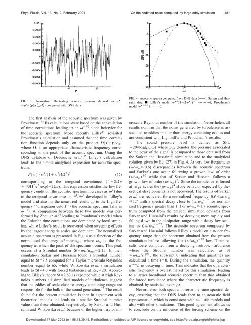
Phys. Fluids, Vol. 13, No. 2, February 2001 On the radiated noise computed by large-eddy simulation FIG. 3. Normalized fluctuating acoustic pressure defined as p* 2 2 p/(u rmsM 0) computed with DNS data. The first analysis of the acoustic spectrum was given by Proudman. 19 His calculations were based on the cancellation of time correlations leading to an 7/2 slope behavior for the acoustic spectrum. More recently Lilley 14 revisited Proudman’s calculation and assumed that the time correlation function depends only on the product xy/c 0 , where is an appropriate characteristic frequency corresponding to the peak of the acoustic spectrum. Using the DNS database of Debussche et al., 35 Lilley’s calculation leads to the simple analytical expression for acoustic spectrum: P 4 /1 2 /42 3 27 corresponding to the temporal covariance (12 4/3 2 2 )exp(2). This expression satisfies the low frequency condition the acoustic spectrum increases as 4 due to the temporal covariance on 4 / 4 developed in Lilley’s model and also fits the measured results up to the high frequency ‘‘dissipation cutoff’’ the acoustic spectrum falls as 2 . A comparison between these two models was performed by Zhou et al. 36 leading to Proudman’s model when the Eulerian time correlations are dominated by local straining, while Lilley’s result is recovered when sweeping effects by the largest energetic scales are dominant. The normalized acoustic spectrum is presented in Fig. 4 as a function of the normalized frequency */ m , where m is the frequency at which the peak of the spectrum occurs. This peak occurs at a Strouhal number StL/u rms2.15. In their simulation Sarkar and Hussaini found a Strouhal number equal to St3.5 computed for a Taylor microscale Reynolds number equal to 65, while Witkowska et al.’s simulation leads to St4.0 with forced turbulence at Re 20. According to Lilley’s theory St2.83 is expected while at high Reynolds numbers all simplified models of turbulence suggest that the eddies of scale close to energy containing range are responsible for the bulk of the sound generation. 37 The result found for the present simulation is then in agreement with theoretical models and leads to a smaller Strouhal number value than these obtained, respectively, by Sarkar and Hussaini and Witkowska et al. because of the higher Taylor mi- 481 FIG. 4. Acoustic spectra computed from DNS data ; Sarkar and Hussaini data ; Lilley’s model * 4 (12* 2 ) 3 ; Proudman’s model * 7/2 ••••. croscale Reynolds number of the simulation. Nevertheless all results confirm that the noise generated by turbulence is associated to eddies smaller than energy-containing eddies and are consistent with Lighthill’s and Proudman’s results. The sound pressure level is defined as SPL 20*log(p/p ref) where p ref denotes the pressure associated to the peak of the signal is compared to those obtained from the Sarkar and Hussaini 20 simulation and to the analytical solution given by Eq. 27 in Fig. 4. At very low frequencies (/ m0.6) discrepancies between the acoustic spectrum and Sarkar’s one occur following a growth law of order (/ m) 1/2 while that of Sarkar and Hussaini follows a growth law of order (/ m) 2 . Since the turbulence is forced at large scales the (/ m) 4 slope behavior expected by theoretical developments is not recovered. The results of Sarkar et al. are recovered for a normalized frequency: 0.6/ m 1.7 with a spectral decay close to (/ m) 2 for normalized frequency greater than 1. For / m1.7 acoustic spectrum computed from the present simulation deviates from Sarkar and Hussaini’s results by decaying more rapidly and falling down in the dissipation range with a decay law scaling as (/ m) 7/2 . The acoustic spectrum computed by Sarkar and Hussaini follows Lilley’s model on a wider frequency range than the spectrum obtained from the present simulation before following the (/ m) 7/2 law. Their results were computed from a decaying isotropic turbulence where the Strouhal number was calculated as St L 0 /u 0 rms , the subscript 0 indicating that quantities are calculated a time t0. During the simulation, the quantity u rms /L is decaying in time. This indicates that the characteristic frequency is overestimated for this simulation, leading to a larger broadband acoustic spectrum than that obtained for forced turbulence where the characteristic frequency is obtained by statistical average. Nevertheless both spectra observe the same spectral decay, ensuring that the DNS leads then to an acoustic field representation which is consistent with acoustic models and also with other simulations. This good agreement allows us to conclude on the influence of the forcing scheme on the Downloaded 17 Mar 2003 to 156.18.39.49. Redistribution subject to AIP license or copyright, see http://ojps.aip.org/phf/phfcr.jsp
482 Phys. Fluids, Vol. 13, No. 2, February 2001 Seror et al. TABLE II. Ratio between acoustic intensities. Ī/I I LES /Ī I LES /Ī Bardina’s model noise generation. It strongly modifies the acoustic properties of the lowest resolved frequencies, yielding a 1/2 slope, but the modes located after the kinetic energy spectrum peak are not polluted, leading to the observed good agreement. Since the maximum of noise production is due to modes located after that peak and since we are interested in LES with a cutoff located in the inertial range, the present forcing scheme can be retained. The same conclusion was given by Witkowska. B. A priori evaluation of subgrid scale tensor contribution to Lighthill’s tensor I LES /Ī Liu’s model 16 3 32 3 64 3 16 3 32 3 64 3 16 3 32 3 64 3 16 3 32 3 64 3 0.93 0.97 0.99 0.45 0.75 0.91 0.66 0.90 0.98 0.68 0.96 1.01 To analyze high frequency and subgrid contributions of the acoustic source term to the radiated noise, a comparison between acoustic quantities computed from all parts occurring in the decomposition Eq. 10 has been carried out. In Table II, ratios between the acoustic intensity I computed from the full Lighthill tensor Tij and acoustic intensity Ī computed from the filtered Lighthill tensor T ¯ ij have been evaluated for all grids. These ratios show that the contribution to the full radiated noise generated by the high frequency part of acoustic tensor Tij remains less than 10% in all cases. In Table III ratios between turbulent scales and the mesh size are presented showing that for all values of k c used the integral scale is well resolved, i.e., L. As the noise is generated by scales smaller than the integral scale this condition must be restricted to L/St, where 1/St 0.47 in the present simulation, and according to all values reported in Table III this condition is satisfied on all grids. This ensures that the scales responsible for the noise are well resolved. Comparison between spectra computed from the full Lighthill tensor and the filtered one in Fig. 5 shows that the acoustic spectrum hardly changes when the high frequency part of the acoustic source term is not taken into account. This result is in agreement with those obtained by Seror et al. 17 ensuring that the use of large-eddy simulation is suitable when it is used together with Lighthill’s analogy and when the mesh size satisfies the condition discussed above. The spectral decay of 7/2 is recovered in the same frequency range while discrepancies between acoustic spectra occur for higher frequencies. The acoustic spectrum de- TABLE III. Parameters and characteristic values of the flow. k c 7 15 31 ¯ / 22.44 10.47 5.07 ¯ / 1.31 0.70 0.34 ¯ /L 0.40 0.20 0.10 FIG. 5. Comparison between acoustic spectra computed from: DNS data -; filtered Lighthill’s tensor on 16 3 nodes ; filtered Lighthill’s tensor on 32 3 ••••; filtered Lighthill’s tensor on 64 3 • • • . cays more rapidly when the Strouhal number St6 as larger cutoff wave number values are considered. When the low frequency part of Lighthill’s tensor is taken into account i.e., uiu j the resulting energy spectrum is computed as a function of uG iu i ˆ . In Fig. 6 these spectra are presented showing that the filter does not modify significantly the inertial range where k5/3 slope is recovered in accordance with Lilley’s model and Zhou and Rubinstein 36 calculations. Since the high frequency part of the acoustic source term can be neglected in all cases, the importance of the noise radiated by the subgrid modes must be estimated. It has been shown by Seror et al. 17 that subgrid scale tensor has a significant contribution to the radiated noise. In Table II the ratio between acoustic intensity computed from the resolved Lighthill tensor namely ILES and Ī has been calculated in all cases. A large contribution of intensity generated by the subgrid scales is observed. This contribution reaches 55% for 163 case. In order to resolve the eddies associated to the peak FIG. 6. Comparison between energy spectrum computed from DNS data: E(k) and energy spectrum associated to the filtered Lightill tensor E(k)G (k) on 16 3 nodes; • ••• 32 3 nodes; • • • 64 3 nodes. Downloaded 17 Mar 2003 to 156.18.39.49. Redistribution subject to AIP license or copyright, see http://ojps.aip.org/phf/phfcr.jsp
Page 1 and 2: PHYSICS OF FLUIDS VOLUME 13, NUMBER
Page 3 and 4: 478 Phys. Fluids, Vol. 13, No. 2, F
Page 5: 480 Phys. Fluids, Vol. 13, No. 2, F

On the radiated noise computed by large-eddy simulation

Create successful ePaper yourself

Delete template?

Save as template?