Physique des écoulements turbulents - Centre Acoustique du LMFA ...

Turbulence and Aeroacoustics 

Research team of the Centre Acoustique 

École Centrale de Lyon & LMFA UMR CNRS 5509 

Physique des écoulements turbulents 

MOD 3 e A, ECL’12 & École doctorale MEGA 

Christophe Bailly ‡ & Olivier Marsden 

Université de Lyon, Ecole Centrale de Lyon & LMFA - UMR CNRS 5509 

& ‡ Institut Universitaire de France 

http://acoustique.ec-lyon.fr

1 

Écoulements turbulents 

apparence très désordonnée 

comportement non prévisible 

A short introduction to turbulent flows 

existence de nombreuses échelles spatiales et temporelles 

La turbulence apparaît lorsque la source d’énergie qui met le fluide en mouvement 

est suffisamment intense devant les effets visqueux que le fluide oppose 

pour se déplacer. 

- astrophysique, écoulements géophysiques, aérodynamique externe 

(aéronautique & transports terrestres), combustion, production 

d’énergie, génie des procédés, biomécanique, ... 

- source de bruit (aéroacoustique), propagation des ondes, couplage 

fluide - structure, ... 

Physique des écoulements turbulents @ Christophe Bailly – ECL’12

2 


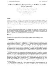
Simulation d’une région de l’Univers de 500 millions d’années-lumière de côté 

‘Horizon project’, Cosmological hydrodynamics 

Institut d’Astrophysique de Paris (Pichon) & CEA (Teyssier) 

Physique des écoulements turbulents @ Christophe Bailly – ECL’12 

Numerical simulation of structure 

formation in an expanding 

universe : N body simulation 

(red temperature) with 70 billions 

particles

3 


Images satellites : météorologie www.meteofrance.com 


www.meteo-lyon.net

4 

Cyclone Ivan - 13 sept. 2004 - catégorie 5 


Cyclone Ivan menançant Cuba et la Floride, progressant à une vitesse de 

14 km/h avec des vents à 260 km/h et des rafales à plus de 354 km/h 


5 

Cyclone Katrina - sept. 2005 - catégorie 5 


vents de 280 km/h en rafale (moyenne sur 1 minute aux USA) 

80% de la Nouvelle-Orléans innondée, see Dixon et al., 2006, Nature, 441, 

586-587 


6 


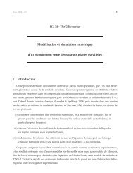
Earth’s surface temperature expressed as anomaly from 1961-90 

(data from www.cru.uea.ac.uk) 

∆T (deg. C) 

0.6 

0.4 

0.2 

0 

−0.2 

−0.4 

−0.6 

−0.8 

1850 1900 1950 2000 

year 

Over both the last 140 years and 100 years, the best estimate is that the global 

average surface temperature has increased by 0.6 ± 0.2 o C. 


7 


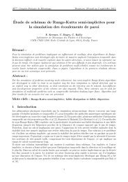
Near-surface wind speeds 10 meters above the Atlantic Ocean 

Data collected by the SeaWinds scatterometer on-board NASA’s QuikSCAT satellite 

(NASA’s Jet Propulsion Laboratory) 


8 

Jupiter’s Great Red Spot (NASA) 



9 


Eruption of the subglacial Grimsvötn volcano, Iceland, on 21 May 2011 

An initial large plume of smoke and ash rose up to about 17 km height. 

Courtesy of Thördïs Högnadóttir, Institute of Earth Sciences, University of Iceland 


10 

Hydrodynamics 



11 

Aeronautics 

Tip vortex behind an airplane 



Fleet Air Arm Corsair III in 1944, 

(unintended) visualization of the 

propeller wake 

Boeing 767-370/ER

12 


Expérience de Reynolds (1883) : régime laminaire / régime turbulent 


13 

Paramètre de contrôle : nombre de Reynolds 

ReD = 


temps diffusion 

temps convection ∼ D2 /ν 

D/Ud 

transition laminaire - turbulent pour ReD = ρUdD 

µ = UdD 

D ∼ distance caractéristique cisaillement 

On doit à Boussinesq (1872, 1877) et 

à Reynolds (1883, 1894) cette définition 

d’un régime turbulent par opposition 

à un régime laminaire. 

Osborn Reynolds 

(1842-1912) 


ν 

∼ 2300 

Joseph Boussinesq 

(1842-1929)

14 

Skin-friction coefficient Cf for a circular pipe 

Cf 

10 0 

10 −1 

10 −2 

10 −3 

10 0 

10 2 

10 4 

ReD = UdD/ν 

laminar regime Cf = 16/ReD 


10 6 

Blasius’ relationship, Cf ≃ 0.0791 Re −1/4 

D 

1/C 1/2 

f 

≃ 3.860 log 10 (ReD C 1/2 

f ) − 0.088 

10 8 


• Oregon facility 

Princeton Superpipe 

McKeon et al. (2004)

15 


Relation between the skin-friction coefficient Cf and the friction coefficient ψ 

(coefficient de frottement local et coefficient de perte de charges) 

p1 

τw = µ dU 

dr 

✻ 

❄ 

D 

 

 

 

 

r=R 

∆p ≡ p1 − p2 = 4cf 

p2 

Cf ≡ τw 

1 

2 ρU2 d 

 

Σ 

∆p ≡ ψ L 

D 

 

ρu·(u · n) dΣ = − 

0 = (−p1 + p2) πD2 

4 

L 1 

D 2 ρU2 d = ψ L 1 

D 2 ρU2 d 


Σ 

1 

2 ρU2 d 

 

pndΣ+ τ(n)dΣ 

Σ 

+ πDL µdU 

dr 

ψ ≡ 4cf 

 

 

 

 

r=R

16 


Zero-pressure-gradient boundary layer on a flat plate 

x2 

O 

∂U1 

U1 

∂x1 

✻ 

❍❍ 

∂U1 

+ U2 

∂x2 

L 

δ 

✻ 

✲ 

∼ ν ∂2 U1 

∂x 2 2 

Ue1 

convection molecular diffusion 

δ 

L ∼ 

1 

√ UL/ν 

✲ 

✲ 

✲ 

✲ 

✲ 

U1 (x2) 

U 2 

L 

∼ ν U 

δ 2 

parabolic laminar boundary layer 


✲ 

x1 

δ2 ν 

∼ 

L2 UL

17 


Couche limite laminaire : solution autosimilaire de Blasius (1908) 

δ 

x1 

≃ 4.92 

δ ≃ 4.92 

1 

Rex 1 

νx1 

Ue1 

x 2 /δ 

1.5 

1.0 

0.5 

Coefficient de frottement local, 

Cf = τw 

1 

2 ρU2 e1 

0.0 0.2 0.4 0.6 0.8 1.0 

U /U 

1 e1 

∼ µU 

δ 

ρU 

2 ∼ ν 

δU 

∼ 1 

Re 1/2 

L 


H. Blasius (1883-1970) 

Cf ≃ 0.664 

Rex 1

18 

Couche limite : transition 


Le régime laminaire est observé jusqu’à un nombre de Reynolds critique d’environ 

Rex 1 = x1Ue1 

ν 

≃ 3.2 × 105 

soit encore, pour un nombre de Reynolds construit sur l’épaisseur de la couche 

limite δ, Reδ = δUe1/ν ≃ 2800. 

turbulent spot growing by destabilizing the 

surrounding laminar flow 


visualization by laser-induced fluorescence (LIF) 

Gad-el-Hak et al. (1981)

19 

Turbulent boundary layer 

F. Laadhari (LMFA) 


Reδ θ ≃ 1000 Ue1 = 2.1 m.s −1 δ ≃ 7 cm uτ ≃ 0.1 m.s −1 x1 ≃ 3 m 

temps convection 

L 

U 

✲ 

convection 

∼ δ 

u ′ temps diffusion turbulente 

Typiquement u ′ /Ue1 ∼ 10 −2 , difficile d’estimer Cf dimensionnellement. 


✻ 

diffusion 

turbulente

20 

Automotive industry 



Posson & Pérot, AIAA Paper 2006-2719

21 


Free shear flows : subsonic turbulent jets Reynolds number ReD = ujD/ν 

Prasad & Sreenivasan (1989) 

ReD ≃ 4000 

Kurima, Kasagi & Hirata (1983) 

ReD ≃ 5.6 × 10 3 

Ayrault, Balint & Schon (1981) 

ReD ≃ 1.1 × 10 4 

Dimotakis et al. (1983) 

ReD ≃ 10 4 


Mollo-Christensen (1963) 

ReD = 4.6 × 10 5

22 

Free shear flows : jets 

visualization with smoke wires 

ReD ≃ 5.4 × 10 4 

Courtesy of H. Fiedler (1987) 


entrainment by a turbulent round jet from a wall 

ReD = 10 6 

Florent, J. Méc. (1965) 


23 


Free shear flows : wake behind a circular cylinder / Karman vortex street 

ReD = 0.16 ReD = 1.54 

ReD = 26 ReD = 138 


24 



Van Dyke, An album of fluid motion 

ONERA - DAFE 

ReD = 140 ReD = 10000 




Alexander Selkirk Island in the southern 

Pacific Ocean. 

25 

← 

→ 

These Karman vortices formed over the 

islands of Broutona, Chirpoy, and Brat 

Chirpoyev ("Chirpoy’s Brother"), all part 

of the Kuril Island chain found between 

Russia’s Kamchatka Peninsula and Ja- 

pan. 


26 

Free shear flows : wakes 


Béguier & Fraunié, Int. J. of Heat and Mass Transfert (1991) 


27 

Non-linéarité des équations de Navier-Stokes 

ρ 

∂u 

∂t 


 

+ u · ∇u 

= −∇p + µ∇ 2 u 

Le terme d’accélération convective u · ∇u est à l’origine des nombreuses échelles 

que l’on observe dans un écoulement turbulent 

Petit exemple illustrant la création d’harmoniques. En notant u = (u, v) 

⎧ 

⎪⎨ 

⎪⎩ 

∂u 

∂t 

∂v 

∂t 

+ u∂u 

∂x 

+ u∂v 

∂x 

+ v ∂u 

∂y 

+ v ∂v 

∂y 

= 0 

= 0 

avec 

⎧ 

⎪⎨ 


⎪⎩ 

u (x, y, t0) = A cos(kxx) cos(kyy) 

v (x, y, t0) = A ′ cos(k ′ x x) cos(k′ y y)

28 



u (x, y, t) = u (x, y, t0) + (t − t0) ∂u 

 

 

 

∂t 

 

∂u 

= − u 

∂t 

∂u 

 

∂u 

+ v 

∂x ∂y 

u (x, y, t) = A cos(kxx) cos(kyy) + (t − t0) 

kyAA ′ 

t0 

kxA 2 

4 

t 0 

t0 

+ ... 

sin(2kxx) cos(2kyy) + 1 

+ (t − t0) {cos [(kx − k 

4 

′ x)x] + cos [(kx + k ′ x)x]} 

× sin (ky − k ′ y)y + sin (ky + k ′ y)y + ... 

On observe la création d’harmoniques supérieures, i.e. de grands nombres d’onde 

ou bien encore de petites structures, et aussi la création de sous-harmoniques. 

Limite pour la taille des plus grands nombres d’onde ou des plus petites structures 

dans un écoulement turbulent ? 


29 



Le transfert vers les grands nombres d’onde est limité par la viscosité moléculaire : 

les particules fluides ne peuvent conserver leur différence de vitesse. 

E(k) spectrum 

energy injection at t 0 

k η 

Plus petites structures : uη kη ∼ 1/lη 

∂u 

∂t ≃ ν∇2 u (Stokes) 

∂u 

∂t ∼ u2 η 

lη 

Reη = lηuη 

ν 

ν∇ 2 u ∼ ν uη 

l 2 η 

Ces échelles (uη, lη) de Kolmogorov, plus petites échelles avant dissipation, ont 

un rôle très important. 


∼ 1

30 


La turbulence est bien du ressort de la mécanique des milieux continus 

lη / λl ? (libre parcours moyen) 

nombre de Knudsen Kn = λl 

lη 

≪ 1 

La non-linéarité des équations de Navier-Stokes ne permet pas de prévoir l’évolution 

du champ turbulent sur des temps très longs : sensibilité aux conditions 

initiales 

(liée à la valeur du plus grand exposant de Lyapunov pour les systèmes dynamiques 

chaotiques) 

Dans l’atmosphère, on estime que deux particules fluides distantes de 10 cm se 

retrouvent séparées d’environ 10 km en une journée, « effet papillon ». 


31 

Blinking vortex flow of Aref (1984) 

x 2 /a 

x 2 /a 

x 2 /a 

0.8 

0 

−0.8 

−1.6 −0.8 0 

x /a 

1 

0.8 1.6 

0.8 

0 

−0.8 

−1.6 −0.8 0 

x /a 

1 

0.8 1.6 

0.8 

0 

−0.8 

−1.6 −0.8 0 

x /a 

1 

0.8 1.6 


β = 0.01 

β = 0.25 

β = 0.40 


for 0 ≤ t ≤ T , vortex (−a, 0) on 

for T ≤ t ≤ 2T , vortex (a, 0) on 

Γ ✲ 

✛ 

2a 

Γ ✲ 

control parameter : β = ΓT 

2πa 2 

chaos in Hamiltonian systems 

(mixing in fluids) 

✲

32 

Role of pressure 

Taking the divergence of the Navier-Stokes equations, 

∂ 

∂xi 

 

ρ 

∂ui 

∂t 

 

∂ui 

+ uj 

∂xj 


= − ∂p 

∂xi 

and p satisfies the Poisson equation, 

∇ 2 p = −ρ ∂ 

∂xi 

 

uj 

+ µ ∂2 ui 

∂x 2 j 

 

∂ui 

∂xj 

 

= −ρ ∂ui 

∂xj 

ρ = cst ∇ · u = 0 

The solution can be explicitly written as, (if p → cst as r → ∞) 

p (x) = ρ 

4π 

 

V 

∂ui ∂uj 

∂yj 

∂yi 

(y) dy 

r 

∂uj 

∂xi 

where r = x − y 

Note that all the points y in the volume V contribute to the pressure at the point 

x, nonlocal relation between velocity and pressure 


33 

Outline of the course 

Découvrir et comprendre la physique des écoulements turbulents 

Établir les bases pour une description statistique indispensable à la modélisation 

Donner un aperçu assez large et pratique de la simulation numérique et des 

techniques expérimentales pour les écoulements turbulents 

introduction aux écoulements turbulents 

description statistique 

écoulements de paroi 

dynamique du tourbillon 

turbulence homogène et isotrope - théorie de Kolmogorov 

aperçu sur la simulation numérique et les techniques expérimentales 


34 

Activités pratiques 

Organisation du cours - ECL 

TP-1 modélisation et simulation d’un écoulement de canal plan 

Centre Acoustique (KCA) 

séance supplémentaire (non inscrits ECL) le jeudi 8 novembre à 14h 

TP-2 anémométrie à fil chaud dans un jet libre 

Mécanique des fluides (I11) 

séance supplémentaire (non inscrits ECL) le jeudi 15 novembre à 14h 

BE – travaux dirigés en petite classe 

vendredi 14 décembre - 13h30 

Étudiants en master, auditeurs libres : 

possibilité de suivre ces activités pratiques : faites vous connaître ! 


35 

Contrôle des connaissances 

4 Exercices (dans une liste au choix 60%) 

+ travail BE (20%) + travaux pratiques (20%) 


Gestion des absences : possible de modifier exceptionnellement une séance de 

TP uniquement en échangeant sa séance avec celle d’un autre étudiant. 

Examen écrit master (MEGA) 

Équipe d’enseignement : Benoît André 

Christophe Bailly 

Christophe Bogey 

Didier Dragna 

Olivier Marsden 


36 


Transparents à télécharger sur le site web du groupe Acoustique, 

http://acoustique.ec-lyon.fr 

merci de NE PAS envoyer vos travaux par mail ! 

Site web à visiter aussi pour sujets de thèses, recherche au LMFA, ... 


37 

Local textbook 

Some references 

Bailly, C. & Comte Bellot, G., 2003 

Turbulence 

CNRS éditions, Paris 

ISBN 2-271-06008-7 

376 pages, 114 figures, 622 references. 

en librairie, prix public : 39 euros 

En vente auprès des auteurs avec 

30% de réduction : 27,50e 


38 

Textbooks 


Batchelor, G.K., 1967, An introduction to fluid dynamics, Cambridge University Press, Cambridge. 

Bailly C. & Comte Bellot G., 2003 Turbulence, CNRS éditions, Paris. 

Candel S., 1995, Mécanique des fluides, Dunod Université, 2nd édition, Paris. 

Davidson P.A., 2004, Turbulence. An introduction for scientists and engineers, Oxford University Press, Oxford. 

Davidson, P.A., Kaneda, Y., Moffatt, H.K. & Sreenivasan, K.R., Edts, 2011, A voyage through Turbulence, Cambridge 

University Press, Cambridge. 

Guyon E., Hulin J.P. & Petit L., 2001, Hydrodynamique physique, EDP Sciences / Editions du CNRS, première édition 

1991, Paris - Meudon. 

Hinze J.O., 1975, Turbulence, McGraw-Hill International Book Company, New York, 1 ère édition en 1959. 

Landau L. & Lifchitz E., 1971, Mécanique des fluides, Editions MIR, Moscou. 

Also Pergamon Press, 2nd edition, 1987. 

Lesieur M., 2008, Turbulence in fluids : stochastic and numerical modelling, Kluwer Academic Publishers, 4th revised 

and enlarged ed., Springer. 

Pope S.B., 2000, Turbulent flows, Cambridge University Press. 

Tennekes H. & Lumley J.L., 1972, A first course in turbulence, MIT Press, Cambridge, Massachussetts. 

Van Dyke M., 1982, An album of fluid motion, The Parabolic Press, Stanford, California. 

White F., 1991, Viscous flow, McGraw-Hill, Inc., New-York, first edition 1974.

Physique des écoulements turbulents - Centre Acoustique du LMFA ...

Create successful ePaper yourself

Delete template?

Save as template?