On the radiated noise computed by large-eddy simulation

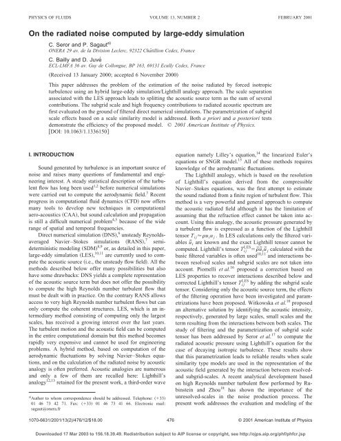
PHYSICS OF FLUIDS VOLUME 13, NUMBER 2 FEBRUARY 2001 

On the radiated noise computed by large-eddy simulation 

C. Seror and P. Sagaut a) 

ONERA 29 av. de la Division Leclerc, 92322 Châtillion Cedex, France 

C. Bailly and D. Juvé 

ECL-LMFA 36 av. Guy de Collongue, BP 163, 69131 Ecully Cedex, France 

Received 13 January 2000; accepted 6 November 2000 

This paper addresses the problem of the estimation of the noise radiated by forced isotropic 

turbulence using an hybrid large-eddy simulation/Lighthill analogy approach. The scale separation 

associated with the LES approach leads to splitting the acoustic source term as the sum of several 

contributions. The subgrid scale and high frequency contributions to radiated acoustic spectrum are 

first evaluated on the ground of filtered direct numerical simulations. The parametrization of subgrid 

scale effects based on a scale similarity model is addressed. Both a priori and a posteriori tests 

demonstrate the efficiency of the proposed model. © 2001 American Institute of Physics. 

DOI: 10.1063/1.1336150 

I. INTRODUCTION 

Sound generated by turbulence is an important source of 

noise and raises many questions of fundamental and engineering 

interest. A steady statistical description of the turbulent 

flow has long been used 1,2 before numerical simulations 

were carried out to compute the aerodynamic field. 3 Recent 

progress in computational fluid dynamics CFD now offers 

many tools to develop new techniques in computational 

aero-acoustics CAA, but sound calculation and propagation 

is still a difficult numerical problem 4,5 because of the wide 

range of spatial and temporal frequencies. 

Direct numerical simulation DNS, 6 unsteady Reynolds- 

averaged Navier–Stokes simulations RANS, 7 

semi- 

deterministic modeling SDM 8,9 or, as detailed in this paper, 

large-eddy simulation LES, 10,11 are currently used to compute 

the acoustic source i.e., the unsteady flow field. All the 

methods described below offer many possibilities but also 

have some drawbacks: DNS yields a complete representation 

of the acoustic source term but does not offer the possibility 

to compute the high Reynolds number turbulent flow that 

must be dealt with in practice. On the contrary RANS allows 

access to very high Reynolds number turbulent flows but can 

only compute the coherent structures. LES, which is an intermediary 

method consisting of computing only the largest 

scales, has received a growing interest over the last years. 

The turbulent motion and the acoustic field can be computed 

in the entire computational domain but this method becomes 

rapidly very expensive and cannot be used for engineering 

problems. A hybrid method, based on computation of the 

aerodynamic fluctuations by solving Navier–Stokes equations, 

and on the calculation of the radiated noise by acoustic 

analogy is often preferred. Acoustic analogies are numerous 

and only a few of them are recalled here: Lighthill’s 

analogy 12,13 retained for the present work, a third-order wave 

a Author to whom correspondence should be addressed. Telephone: 33 

01 46 73 42 71. Fax: 33 01 46 73 41 66. Electronic mail: 

sagaut@onera.fr 

equation namely Lilley’s equation, 14 the linearized Euler’s 

equations or SNGR model. 15 All of these methods requires 

knowledge of the aerodynamic fluctuations. 

The Lighthill analogy, which is based on the resolution 

of Lighthill’s equation derived from the compressible 

Navier–Stokes equations, was the first attempt to estimate 

the sound radiated from a finite region of turbulent flow. This 

method is a very powerful and general approach to compute 

the acoustic radiated field although it has the limitation of 

assuming that the refraction effect cannot be taken into account. 

Using this analogy, the acoustic pressure generated by 

a turbulent flow is expressed as a function of the Lighthill 

tensor Tiju iu j . In LES calculations only the filtered variables 

ũi are known and the exact Lighthill tensor cannot be 

LES 

computed. Lighthill’s tensor Tij ¯ũ iũ j calculated with the 

basic filtered variables is often used 10,11 and interactions between 

resolved scales and subgrid scales are not taken into 

account. Piomelli et al. 16 proposed a correction based on 

LES properties to recover interactions described below and 

LES 

corrected Lighthill’s tensor Tij by adding the subgrid scale 

tensor. Considering only the acoustic source term, the effects 

of the filtering operation have been investigated and parametrizations 

have been proposed. Witkowska et al. 10 proposed 

an alternative solution by identifying the acoustic intensity, 

respectively, generated by large scales, small scales and the 

term resulting from the interactions between both scales. The 

study of filtering and the parametrization of subgrid scale 

tensor has been addressed by Seror et al. 17 to compute the 

radiated acoustic pressure using Lighthill’s equation for the 

case of decaying isotropic turbulence. These results show 

that this parametrization leads to reliable results when scale 

similarity type models are used in the representation of the 

acoustic field generated by the interaction between resolvedand 

subgrid-scales. A recent analytical development based 

on high Reynolds number turbulent flow performed by Rubinstein 

and Zhou 18 has shown the importance of the 

unresolved-scales in the noise production process. The 

present work addresses the evaluation and modeling of the 

1070-6631/2001/13(2)/476/12/$18.00 476 

© 2001 American Institute of Physics 

Downloaded 17 Mar 2003 to 156.18.39.49. Redistribution subject to AIP license or copyright, see http://ojps.aip.org/phf/phfcr.jsp

Phys. Fluids, Vol. 13, No. 2, February 2001 On the radiated noise computed by large-eddy simulation 

unresolved- and subgrid-scales contribution to the radiated 

noise itself when Lighthill’s analogy and LES are used together 

for larger Reynolds number turbulent flows on the 

ground of a priori and a posteriori tests. The case of the 

sound radiated by a volume of isotropic turbulence is retained 

as a test case for the present study. This is an academic 

case, which is one of the very few examples of turbulent 

flow whose equivalent acoustic source has well defined 

properties. It appears consequently as a first step toward the 

derivation of fully general model. This problem has been 

addressed by many authors, both from a theoretical 14,19 and a 

numerical 10,20 point of view. Nevertheless, even for this very 

simple turbulent flow, the authors are not aware of any published 

a posteriori tests for subgrid models for the noise 

source, the previous studies being devoted to a priori analysis. 

Considering that the modeling process for the subgrid 

noise source should start with simple flows, which are well 

controlled from a theoretical and numerical point of view, 

isotropic turbulence appears as an mandatory first step. But, 

as for the modeling of usual subgrid terms, recall that the 

extension to more complex flows could be required to complicate 

the models. This point will be addressed in future 

works. 

The mathematical formulation concerning Lighthill’s 

equation is first presented in Sec. II. Section III is devoted to 

the description of the numerical method and the implementation 

of acoustic calculations for the study. Numerical results 

obtained from a priori tests i.e., filtered DNS and 

concerning both evaluation and modeling of the subgrid 

scale effects are detailed in Sec. IV. In order to assess conclusions 

given by the filtered DNS, a posteriori tests described 

in Sec. V have been carried out. Conclusions are 

presented in Sec. VI. 

II. MATHEMATICAL FORMULATION 

A. Governing equations 

Lighthill’s analogy 12,13 is a method to compute the radiated 

acoustic field from a finite region of turbulent flow. This 

analogy is based on a combination of compressible Navier– 

Stokes equations which leads to an inhomogeneous wave 

equation for the density 

2 t 2 c 2 

2 

0 

y iy i 

2 

T 

y 

ij, 1 

iy j 

where c0 is the constant speed of sound in the ambient medium, 

which is supposed to be at rest, and the Lighthill tensor 

Tij is defined as follows: 

T iju iu jpc 0 2 ij ij. 2 

For high Reynolds numbers the viscous stress tensor ij in 

Lighthill’s tensor expression can be neglected. The quantity 

2 21 

(pc 0) is responsible for thermoacoustics effects and 

will be neglected for the class flow that have been considered 

in this paper. Under these assumptions, the Lighthill tensor 

simplifies to 

Tiju iu j . 3 

The solution of the Lighthill equation leads to a representation 

of the radiated acoustic field. Once the acoustic source 

term, which is zero outside the flow region, has been computed 

by solving the Navier–Stokes equations to compute 

variables and u i , the sound field generated by the turbulent 

motion is uniquely defined. This equation has an exact solution 

only for an homogeneous medium at rest, which can be 

obtained using the Green function. For high Reynolds number 

flow, a complete knowledge of the source term requires a 

high resolution of the flow field and then an important computational 

cost. A direct numerical simulation DNS may 

only be applied on simple configurations 22 and is far from 

addressing range of Reynolds number that have to be dealt 

with in practice. 

B. Extension to LES 

When a large-eddy simulation is performed to obtain 

aerodynamic fluctuations, Lighthill’s equation should be derived 

from the filtered Navier–Stokes equations. This formalism 

has been presented by Seror et al. 17 for the compressible 

subsonic case. Since we are dealing with very low 

Mach number turbulent flows, the present simulations have 

been performed using the incompressible Navier–Stokes 

equations. As expressed in Crow’s paper 23 the inconsistent 

incompressible approximation to Lighthill’s source term is 

justifiable for low Mach number turbulent flow. More recently, 

Ristorcelli 24 has shown that the associated error term 

scales as the square of the Mach number. This approximation 

is then appropriate to compute flows which are under consideration 

in the present work. 

In large-eddy simulation of turbulent flows, any quantity 

F in the flow domain V can be split into a resolved or filtered 

part F ¯ and an unresolved or subgrid part f through the application 

of a low-pass convolution filter: 

with 

FF ¯ f , 4 

F¯ y GyFd, 5 

V 

where G is the spatial kernel filter and /k c the characteristic 

cutoff length scale. The cutoff wave number k c 

defines the limit between the low-frequency components resolved 

in the simulation and the remaining high-frequency 

components which are modeled. The kernel G is currently 

represented by a sharp cutoff filter, a Gaussian filter or tophat 

filter for analytical development. This function is assumed 

to fulfill the three following constraints: constant 

preservation, linearity and commutativity with derivatives. A 

filtered Lighthill equation can then be obtained in the following 

two ways: by operating the combination between the 

filtered continuity equation and filtered momentum equation 

used in LES or by filtering the Lighthill equation 1. Both 

methods lead to the equation 

2 

t 2 ¯c 0 2 2 

y iy i 

477 

¯ 2 

T¯ 

y 

ij. 6 

iy j 


478 Phys. Fluids, Vol. 13, No. 2, February 2001 Seror et al. 

Under the assumptions of isentropic acoustic pressure fluctuations 

due to low Mach number and high Reynolds number 

turbulent flow, the filtered Lighthill tensor T ¯ ij which represents 

the production of resolved acoustic fluctuations is then 

given by 

T¯ 

iju iu j 0u iu j, 7 

where 0 is the flow density. As only the filtered velocity 

components ūi are available in LES calculations, the filtered 

Lighthill tensor cannot be computed and must be written as a 

function of filtered variables. Introducing the subgrid scale 

tensor ij resulting from the nonlinearity of the convective 

terms and defined as 

iju iu jū iū j, 8 

LES 

T¯ 

ij can be approximated by Tij 0ū iū j with an inherent 

SGS 

error Tij which is actually the subgrid scale tensor ij defined 

in Eq. 8: 

LES SGS 

TijT ij Tij 0ū iū j ij. 9 

The final decomposition for the full Lighthill tensor is then 

written as 

LES SGS 

TijT ij Tij Tij , 10 

where Tij is the high-frequency part of the Lighthill tensor 

and is not resolved in LES calculations. 

The subgrid scale tensor appears naturally as a source 

term in the expression of the acoustic fluctuating pressure. In 

order to get reliable far-field noise prediction using LES calculations, 

this tensor must be evaluated to assess the accuracy 

of a prediction of the far-field noise from LES simulations. 

III. NUMERICAL ALGORITHM 

A. Numerical method and forcing scheme 

1. Direct numerical simulation 

A direct numerical simulation has been performed on a 

three dimensional incompressible turbulence. The dynamical 

equation of the Fourier-transformed velocity û i(k,t) for 

wave vector k and time t, are written, following Orszag: 25,26 

 

t k2 û ik,t i 

2 P ilmk û lpû mkpdp, 

11 

where 

Pilmkk m ilk ik l /k 2 k l imk ik m /k 2 . 12 

Equation 11 is solved using Rogallo’s 27 pseudospectral algorithm, 

which evaluates the convolution integral by taking 

the product in physical space. This algorithm does introduce 

aliasing errors which can be reduced by filtering the velocity 

field with an appropriate sharp cutoff filter. In the simulation 

the Fourier-transformed convective term components have 

been truncated for the wave number outside a sphere of radius 

2 

3N, where N is the number of grid nodes used in each 

direction. The time integration has been performed using a 

third-order Runge–Kutta scheme. Periodic boundary condi- 

tions are applied to the solution domain which is a cubic box 

of length 2, with N 3 192 3 equispaced grid nodes. 

2. The forcing scheme 

Since we are interested in a spectral analysis of the 

acoustic field, a statistically stationary turbulence is 

required. 10 In decaying isotropic turbulence, kinetic energy is 

dissipated after a few eddy turns over time following the 

t1.2 decay law, 28 leading then to a vanishing acoustic pressure. 

A spectral deterministic forcing scheme has been 

implemented to obtain statistically stationary velocity field. 

One way to generate statistically stationary turbulence is to 

‘‘force’’ the large scale velocity components by artificially 

adding energy. This energy cascades toward the small scales 

and is dissipated by viscous mechanisms. Many forcing 

schemes have been proposed: Siggia and Patterson 29 

‘‘froze’’ the velocity Fourier amplitudes in a low-wave number 

band, and similarly She et al. 30 introduced a scheme to 

maintain the energy in each of the first two wave number 

shells constant in time. Another class of forcing scheme consists 

of adding an acceleration term into the momentum 

equation. 31 The forcing scheme used in the present work has 

been used by Witkowska et al. 10 for a similar study of sound 

radiated by isotropic turbulence. This forcing scheme maintains 

the total kinetic energy at a constant level by injecting 

the energy lost during the dissipation process namely E in 

the normalized wave number band k min ,kmax1,5. The 

resulting forcing scheme reads 

ûn1 kû*k, 13 

where ûn1 (k) is the Fourier coefficient at time (n1)t 

and û*(k) the Fourier coefficient computed by integrating 

the Navier–Stokes equation with ûn (k) as an initial condition, 

with 

1E kmax Ekdk kk min ,k max 

kmin 

, 

1 otherwise 

14 

where E is the kinetic energy loss due to dissipation during 

the time t. According to Witkowska et al. 10 this method 

ensures the continuity of the second-order derivatives in 

time, preventing spurious noise generation. This condition is 

indeed required for the present simulations: as will be shown 

in the following sections the acoustic source term can be 

expressed as a function of the second-order time-derivative 

of the Lighthill tensor, and the continuity of this derivative is 

then required. 

Furthermore as the large-eddy simulation is based on 

parametrization of the small scales it is necessary that the 

small scales do not depend on the forcing scheme. The 

present forcing scheme appears as a post-processing of the 

velocity field computed after each time step, and does not 

appear explicitly neither in the momentum equation nor in 

the Lighthill equation. Its exact impact on noise production 

cannot be a priori analyzed, and will be discussed a posteriori 

when presenting DNS results see Sec. IV A. 



B. Implementation of a priori and a posteriori tests 

for LES 

To compute the contributions of the tensors appearing in 

the decomposition of the Lighthill tensor, a priori tests have 

been carried out by filtering the flow field computed with a 

direct numerical simulation. A Gaussian filter function has 

been used for the present simulation, whose associated kernel 

in physical space G and transfer function G ˆ are, respectively, 

Gy 6 

2 

1/2 

exp 6y 

2 2 

Gˆ k 

exp 2 k 2 

24 . 15 

This Gaussian filter induces a smooth separation between 

resolved and subgrid quantities, resulting in a nonzero contribution 

of low frequencies to the latters. The effects of the 

filter have been investigated for three values of the normalized 

wave number k c (k c7,15,31) leading to a representation 

of the field on 16 3 ,32 3 and 64 3 grids, respectively. A 

large-eddy simulation using a parametrization of the subgrid 

scale tensor occurring in the Navier–Stokes equation is performed 

to complete the study with a posteriori tests. Aerodynamic 

fluctuations generated by stationary turbulence may 

be computed by resolving incompressible Navier–Stokes 

equations which are written as 

 

t ūi 

ū 

y 

iū j 

j 

 

y i 

 

p¯ 

y i 

 

y j 

 

ū 

y 

j 

i 

 

ū 

y i 

j 

 

 

y 

ij, 16 

j 

ū i0, 17 

where ij is the subgrid scale tensor. Then the radiated noise 

is deduced using the filtered Lighthill equation 6 where the 

associated Lighthill tensor is given by T ¯ ij 0(ū iū j ij). 

The subgrid scale tensor parametrization is required in 

momentum and Lighthill’s equation but this parametrization 

is not required to be the same for both equations. It is worth 

noting that the subgrid terms appearing in these two equations 

correspond to very different physical mechanism classical 

inter-scale interactions in the momentum equation and 

noise production for the Lighthill source term which are 

associated to different mathematical formulations: simple divergence 

of the subgrid tensor in the momentum equations, 

and a second-order derivative of the same tensor in the 

Lighthill equation. It appears then that different models can 

be derived for these two terms. A ‘‘perfect’’ model for the 

subgrid fluctuations or the subgrid tensor ij could theoretically 

be used to parametrize both effects, but previous works 

by Seror et al. 17 have shown that such a model remains to be 

derived. Two different models will be used in the present 

study. The spectral models used in momentum equations developed 

by Métais and Lesieur 32 leads to the subgrid scale 

tensor 

FIG. 1. Geometry of sound source radiation. VVolume of turbulent fluid, 

Mobserver position, D2. 

ijt 

ū 

y 

j 

i 

 

ū 

y i , 18 

j 

where t(k) (k) is the turbulent viscosity. The effective 

viscosity is written as follows: 

k1 K 0 3/2 

15.2 exp3.03kc /k. 19 

Métais and Lesieur 32 developed a spectral dynamic model to 

compute the eddy viscosity based on an adaptation of the 

spectral-cusp model to kinetic-energy spectra proportional to 

km . The eddy viscosity is then such as 

0.31 5m 

m1 K 0 3/2 Ek c 

k c 

if m3. 20 

For m3 the eddy viscosity is set equal to zero. 

C. Implementation of Lighthill’s analogy 

The acoustic field is evaluated from Lighthill’s analogy. 

The source term is assumed to be nonzero only in a finite 

region V. Then for any observer defined by the vector x, and 

located outside this volume V as shown in Fig. 1, application 

of the Green’s function formalism yields 

x,t 1 1 

2 4c 0 

Vxy 

2 

T 

y 

ij y,t 

iy j 

xy 

c d 

0 3y, 21 

where is the averaged density outside the flow domain V. 

This ensemble average is performed over 24 different 

observers located at the same distance from the center of the 

computational domain. As detailed by Witkowska 10 and Bastin 

et al. 7 three formulations of the solution can be expressed 

from Eq. 21. The formulation retained for the present work 

is the one successfully used by Witkowska 10 and Sarkar and 

Hussiani 20 in isotropic turbulence formulation and which is 

derived from Eq. 21 by applying the divergence theorem 

twice: 33 

x,t 1 xix j 2 d3y. 4c 0 4 

x 3 V 

t 2 Tij y,t xy 

c 0 

Downloaded 17 Mar 2003 to 156.18.39.49. Redistribution subject to AIP license or copyright, see http://ojps.aip.org/phf/phfcr.jsp 

479 

22


FIG. 2. Normalized energy spectrum defined as: E*E(k)/ 0 E(k)]dk presented 

for three different times: t*10.6, t*20.5, t*35.4, the 

full line represents k 5/3 . 

Following the previous results presented in Refs. 10 and 20, 

boundary contributions appearing in Eq. 22 are suppressed 

in order to suppress spurious contributions due to the truncation 

of the source volume. This technique was shown in 

these references to yield very satisfactory results when computing 

the noise radiated by a volume of isotropic turbulence. 

IV. NUMERICAL RESULTS 

A. Direct numerical simulation 

The velocity components have been initialized with 

Gaussian random numbers with the following initial energy 

spectrum: 

Ekk 4 exp2k 2 2 

/k 0 where k04. 23 

The forcing scheme has been implemented after allowing the 

turbulence to decay until an arbitrary time ensuring that a 

self-similar solution is reached. The steady state is obtained 

at the dimensionless time t*t/10.63, where L/u rms 

4.05 denotes the eddy turn over time. Acoustic computations 

have been carried out over approximately 25 eddy turn 

over time. The normalized energy spectrum is presented in 

Fig. 2 for three different times, which represent the initial 

time for acoustic computations, an intermediary time and the 

final time of the simulation, ensuring that the stationary state 

is obtained. The factor kmax1.26, where ( 3 /) 1/4 is 

the Kolmogorov length scale, ensures that the small scales 

are well resolved 34 and a k5/3 slope is recovered on the 

interval 4k18. The time averaged skewness factor of the 

velocity derivative equals 0.47 oscillating between values 

0.46 and 0.5. Since the experimental value is given to be 

0.4, while simulations give Sk0.5, the result leads to a 

satisfactory agreement. Time averaged statistical turbulent 

quantities have been computed in terms of the three dimensional 

energy spectrum E(k). The instantaneous energy dissipation 

rate, , is computed as follows: 

TABLE I. Parameters and characteristic values of the flow for each simulation. 

Simulation N Re u rms L 

DNS 192 82.31 0.25 0.98 0.28 0.02 

case 1 48 ¯ 0.235 1.06 ¯ ¯ 

case 2 96 ¯ 0.242 0.99 ¯ ¯ 

case 3 48 ¯ 0.34 1.11 ¯ ¯ 

case 4 96 ¯ 0.23 1.06 ¯ ¯ 

case 5 192 ¯ 0.23 1.05 ¯ ¯ 

 

2 k 

0 

2Ekdk 24 

and the squared rms velocity is written as 

2 

2 

urms Ekdk. 25 

3 0 

Other length scales used in this paper are the integral length 

scale L and the Taylor microscale defined as 

L 1 

2 2u rms 

0 k Ekdk and 215 u rms 

. 26 

 

The Taylor microscale Reynolds number Reurms/ remains 

close to 82 during all the simulation. All averaged 

characteristic values and length scales are presented in 

Table I. 

Lilley 14 emphasized some requirements for studying 

noise produced by isotropic turbulence at low Mach numbers 

on the grounds of previous works by Proudman. The first 

requirement is that no anisotropic effects are present in the 

flow. Considering the case of a volume of isotropic turbulence 

of size D immersed in a laminar infinite space, he 

recommended L/D1. It is observed see Table I that the 

integral length scale L is very close to 1 in all the presented 

simulations, with D2. This corresponds to the usual 

value of the ratio L/D where D is the size of the computational 

domain see Eswaran and Pope 34 and Overholt and 

Pope 31 for a large number of examples, ensuring that the 

two-point correlations decay fast enough to prevent spurious 

coupling of the fluctuations. Because of the triperiodic nature 

of the simulation, there is no boundary effect between turbulence 

and a laminar zone, rendering the constraint less stringent 

than in the case considered by Lilley. The second requirement 

is that the turbulence must not decay significantly 

in the time the sound takes to cross the turbulent region, 

yielding ML/D. In our case, since the turbulence is forced 

and does not decay, that constraint is automatically satisfied. 

The radiated fluctuating acoustic pressure p(x,t) 

2 

c 0((x,t)) is then computed using DNS data by 

solving Eq. 22. The normalized fluctuating acoustic pres- 

2 2 

sure p*p/(urmsM 0), where M 0u rms /c 00.074 is the 

averaged Mach number associated to the propagation outside 

the domain is presented in Fig. 3 as a function of the normalized 

time t*t/ at an observer location. The signal corresponds 

to a general steady process rendering possible a 

spectral analysis of the acoustic pressure. 

Downloaded 17 Mar 2003 to 156.18.39.49. Redistribution subject to AIP license or copyright, see http://ojps.aip.org/phf/phfcr.jsp 

2


FIG. 3. Normalized fluctuating acoustic pressure defined as p* 

2 2 

p/(u rmsM 

0) computed with DNS data. 

The first analysis of the acoustic spectrum was given by 

Proudman. 19 His calculations were based on the cancellation 

of time correlations leading to an 7/2 slope behavior for 

the acoustic spectrum. More recently Lilley 14 

revisited 

Proudman’s calculation and assumed that the time correlation 

function depends only on the product xy/c 0 , 

where is an appropriate characteristic frequency corresponding 

to the peak of the acoustic spectrum. Using the 

DNS database of Debussche et al., 35 Lilley’s calculation 

leads to the simple analytical expression for acoustic spectrum: 

P 4 /1 2 /42 3 27 

corresponding to the temporal covariance (12 

4/3 2 2 )exp(2). This expression satisfies the low frequency 

condition the acoustic spectrum increases as 4 due 

to the temporal covariance on 4 / 4 developed in Lilley’s 

model and also fits the measured results up to the high frequency 

‘‘dissipation cutoff’’ the acoustic spectrum falls as 

2 . A comparison between these two models was performed 

by Zhou et al. 36 leading to Proudman’s model when 

the Eulerian time correlations are dominated by local straining, 

while Lilley’s result is recovered when sweeping effects 

by the largest energetic scales are dominant. The normalized 

acoustic spectrum is presented in Fig. 4 as a function of the 

normalized frequency */ m , where m is the frequency 

at which the peak of the spectrum occurs. This peak 

occurs at a Strouhal number StL/u rms2.15. In their 

simulation Sarkar and Hussaini found a Strouhal number 

equal to St3.5 computed for a Taylor microscale Reynolds 

number equal to 65, while Witkowska et al.’s simulation 

leads to St4.0 with forced turbulence at Re 20. According 

to Lilley’s theory St2.83 is expected while at high Reynolds 

numbers all simplified models of turbulence suggest 

that the eddies of scale close to energy containing range are 

responsible for the bulk of the sound generation. 37 The result 

found for the present simulation is then in agreement with 

theoretical models and leads to a smaller Strouhal number 

value than these obtained, respectively, by Sarkar and Hussaini 

and Witkowska et al. because of the higher Taylor mi- 

481 

FIG. 4. Acoustic spectra computed from DNS data ; Sarkar and Hussaini 

data ; Lilley’s model * 4 (12* 2 ) 3 ; Proudman’s 

model * 7/2 ••••. 

croscale Reynolds number of the simulation. Nevertheless all 

results confirm that the noise generated by turbulence is associated 

to eddies smaller than energy-containing eddies and 

are consistent with Lighthill’s and Proudman’s results. 

The sound pressure level is defined as SPL 

20*log(p/p ref) where p ref denotes the pressure associated 

to the peak of the signal is compared to those obtained from 

the Sarkar and Hussaini 20 simulation and to the analytical 

solution given by Eq. 27 in Fig. 4. At very low frequencies 

(/ m0.6) discrepancies between the acoustic spectrum 

and Sarkar’s one occur following a growth law of order 

(/ m) 1/2 while that of Sarkar and Hussaini follows a 

growth law of order (/ m) 2 . Since the turbulence is forced 

at large scales the (/ m) 4 slope behavior expected by theoretical 

developments is not recovered. The results of Sarkar 

et al. are recovered for a normalized frequency: 0.6/ m 

1.7 with a spectral decay close to (/ m) 2 for normalized 

frequency greater than 1. For / m1.7 acoustic spectrum 

computed from the present simulation deviates from 

Sarkar and Hussaini’s results by decaying more rapidly and 

falling down in the dissipation range with a decay law scaling 

as (/ m) 7/2 . The acoustic spectrum computed by 

Sarkar and Hussaini follows Lilley’s model on a wider frequency 

range than the spectrum obtained from the present 

simulation before following the (/ m) 7/2 law. Their results 

were computed from a decaying isotropic turbulence 

where the Strouhal number was calculated as St 

L 0 /u 0 rms , the subscript 0 indicating that quantities are 

calculated a time t0. During the simulation, the quantity 

u rms /L is decaying in time. This indicates that the characteristic 

frequency is overestimated for this simulation, leading 

to a larger broadband acoustic spectrum than that obtained 

for forced turbulence where the characteristic frequency is 

obtained by statistical average. 

Nevertheless both spectra observe the same spectral decay, 

ensuring that the DNS leads then to an acoustic field 

representation which is consistent with acoustic models and 

also with other simulations. This good agreement allows us 

to conclude on the influence of the forcing scheme on the 



TABLE II. Ratio between acoustic intensities. 

Ī/I I LES /Ī 

I LES /Ī 

Bardina’s model 

noise generation. It strongly modifies the acoustic properties 

of the lowest resolved frequencies, yielding a 1/2 slope, but 

the modes located after the kinetic energy spectrum peak are 

not polluted, leading to the observed good agreement. Since 

the maximum of noise production is due to modes located 

after that peak and since we are interested in LES with a 

cutoff located in the inertial range, the present forcing 

scheme can be retained. The same conclusion was given by 

Witkowska. 

B. A priori evaluation of subgrid scale tensor 

contribution to Lighthill’s tensor 

I LES /Ī 

Liu’s model 

16 3 32 3 64 3 16 3 32 3 64 3 16 3 32 3 64 3 16 3 32 3 64 3 

0.93 0.97 0.99 0.45 0.75 0.91 0.66 0.90 0.98 0.68 0.96 1.01 

To analyze high frequency and subgrid contributions of 

the acoustic source term to the radiated noise, a comparison 

between acoustic quantities computed from all parts occurring 

in the decomposition Eq. 10 has been carried out. 

In Table II, ratios between the acoustic intensity I computed 

from the full Lighthill tensor Tij and acoustic intensity 

Ī computed from the filtered Lighthill tensor T ¯ ij have been 

evaluated for all grids. These ratios show that the contribution 

to the full radiated noise generated by the high fre- 

quency part of acoustic tensor Tij remains less than 10% in 

all cases. In Table III ratios between turbulent scales and the 

mesh size are presented showing that for all values of k c 

used the integral scale is well resolved, i.e., L. As the 

noise is generated by scales smaller than the integral scale 

this condition must be restricted to L/St, where 1/St 

0.47 in the present simulation, and according to all values 

reported in Table III this condition is satisfied on all grids. 

This ensures that the scales responsible for the noise are well 

resolved. Comparison between spectra computed from the 

full Lighthill tensor and the filtered one in Fig. 5 shows that 

the acoustic spectrum hardly changes when the high frequency 

part of the acoustic source term is not taken into 

account. This result is in agreement with those obtained by 

Seror et al. 17 ensuring that the use of large-eddy simulation 

is suitable when it is used together with Lighthill’s analogy 

and when the mesh size satisfies the condition discussed 

above. 

The spectral decay of 7/2 is recovered in the same 

frequency range while discrepancies between acoustic spectra 

occur for higher frequencies. The acoustic spectrum de- 

TABLE III. Parameters and characteristic values of the flow. 

k c 7 15 31 

¯ / 22.44 10.47 5.07 

¯ / 1.31 0.70 0.34 

¯ /L 0.40 0.20 0.10 

FIG. 5. Comparison between acoustic spectra computed from: DNS data -; 

filtered Lighthill’s tensor on 16 3 nodes ; filtered Lighthill’s tensor 

on 32 3 ••••; filtered Lighthill’s tensor on 64 3 • • • . 

cays more rapidly when the Strouhal number St6 as larger 

cutoff wave number values are considered. When the low 

frequency part of Lighthill’s tensor is taken into account 

i.e., uiu j the resulting energy spectrum is computed as a 

function of uG iu i 

ˆ . In Fig. 6 these spectra are presented 

showing that the filter does not modify significantly the inertial 

range where k5/3 slope is recovered in accordance 

with Lilley’s model and Zhou and Rubinstein 36 calculations. 

Since the high frequency part of the acoustic source term 

can be neglected in all cases, the importance of the noise 

radiated by the subgrid modes must be estimated. It has been 

shown by Seror et al. 17 that subgrid scale tensor has a significant 

contribution to the radiated noise. In Table II the 

ratio between acoustic intensity computed from the resolved 

Lighthill tensor namely ILES and Ī has been calculated in 

all cases. A large contribution of intensity generated by the 

subgrid scales is observed. This contribution reaches 55% for 

163 case. In order to resolve the eddies associated to the peak 

FIG. 6. Comparison between energy spectrum computed from DNS data: 

E(k) and energy spectrum associated to the filtered Lightill tensor 

E(k)G (k) on 16 3 nodes; • ••• 32 3 nodes; • • • 64 3 

nodes. 



FIG. 7. Comparison between acoustic pressures respectively associated to 

the filtered Lighthill tensor and the resolved Lighthill tensor 

on 32 3 grid. 

of the acoustic spectrum the condition /L0.471/St is 

required, for this grid (16 3 )/L0.4 is obtained indicating 

that the smallest resolved eddies are very close to those associated 

to the peak of the acoustic spectrum. 

When the subgrid scale effects representing the interaction 

between the resolved and the unresolved structures are 

not taken into account, the results obtained are very far from 

the solution computed from the low frequency part of the 

acoustic source term. The largest error is observed as expected 

for the lowest value of k c i.e., 16 3 used for the 

simulation. On the 32 3 grid mesh representation presented in 

Fig. 7, the subgrid contribution is still significant. Errors occur 

for both amplitude and phase of the acoustic signal indicating 

an important effect of the subgrid scale. 

The comparison between acoustic spectra of the quantity 

(p/p ref) 2 where p ref is the amplitude of the peak of the spectrum 

for DNS case and the pressure p is computed from the 

full Lighthill tensor and from the resolved one is presented in 

Fig. 8. Important discrepancies concerning acoustic spectrum 

computed on 16 3 and 32 3 grids occur while the solution on 

FIG. 8. Comparison between acoustic spectra computed from: the full 

Lighthill tensor ; the resolved Lighthill tensor on 16 3 , on 

32 3 ••••, on64 3 • • • grids. 

FIG. 9. Comparison between energy spectrum computed from DNS data: 

E(k) and energy spectrum associated to the filtered Lightill tensor 

E(k)G 2 (k) on 16 3 nodes; • ••• 32 3 nodes; • • • 64 3 

nodes. 

64 3 nodes remains close to the DNS result. As the filtered 

Lighthill tensor allows to recover the behavior expected by 

Proudman’s theory, the resolved Lighthill tensor does not for 

the two lowest values of k c as shown in Fig. 8. In the frequency 

range St2,6 where Proudman’s model was recovered, 

the acoustic spectrum decreases more rapidly when the 

resolved Lighthill tensor is used for the computation. Moreover 

the peak of the acoustic spectrum for these two cases 

has been shifted to the lowest frequency leading now to St 

1.8 for the 16 3 case and a 2.0 for the 32 3 case while St 

2.15 was expected Fig. 8. As suggested by the intensity 

ratio I LES /Ī0.91 on the 64 3 grid the acoustic spectrum remains 

close to the DNS one. When a LES is performed the 

resulting kinetic energy spectrum is computed as a function 

of u iu jG ˆ 2 . These spectra are presented in Fig. 9 showing 

that the inertial range is still there for cutoff wave number 

values considered. As the decay of Eulerian time correlations 

was dominated by large scale straining according to Zhou 

et al., 36 the use of the resolved Lighthill tensor does not recover 

reliable results indicating that the subgrid scale tensor 

should be parametrized in both cases 16 3 and 32 3 mesh grid 

to get reliable results for the acoustic field. 

C. Parametrization of the Lighthill subgrid scale 

tensor 

483 

In order to recover reliable results concerning both 

acoustic intensity and Strouhal number when LES and Lighthill’s 

tensor are used together, a parametrization of the subgrid 

Lighthill tensor must be performed. Two models have 

been tested for the compressible case: 17 a subgrid scale 

model of eddy viscosity type, like the Smagorinsky model 38 

and a scale similarity type model, like the Bardina 

model. 39,40 The Bardina model led to better results than the 

Smagorinsky model and for the present simulations scale 

similarity models have been retained. Subgrid Lighthill’s 

tensor parametrization with Bardina’s model has been chosen 

leading to 



FIG. 10. Comparison between acoustic spectra computed from DNS data and filtered DNS on 16 3 nodes a and 32 3 nodes b: the full Lighthill tensor ; 

the resolved Lighthill tensor ; the resolved Lighthill tensor with a correction given by Bardina’s model • •••; the resolved Lighthill tensor with 

a correction given by Liu’s model • • • . 

SGS 

Tij mijū iū ju iu j . 28 

The Bardina model is indeed a theoretical model, which cannot 

be applied if the analytical form of the filter is unknown. 

Liu et al. 41 have developed a more general scale similarity 

model written as follows: 

mijC Lū ū iū j 

˜ iū ˜ j, 29 

where CL0.45, bar still denotes a filter at scale ¯ associated 

to the mesh size and tilde denotes a filter at scale 2¯ . 

The ratio between the acoustic intensity computed from 

the resolved Lighthill tensor corrected with subgrid tensor 

namely ILES and the filtered acoustic intensity is presented 

in Table II. In all cases and for both models significant improvements 

are observed. Nevertheless Liu’s model seems to 

recover better results than Bardina’s one. The ratio reaches 

96% and more than 99% for, respectively, 323 and 643 grid 

nodes confirming that scale similarity models are suitable to 

recover the noise generated by the subgrid scales. Acoustic 

spectra computed from the full Lighthill tensor, the resolved 

Lighthill tensor and the resolved Lighthill tensor corrected 

with both models are presented in Figs. 10a and 10b, 

respectively, for the 163 grid and the 323 grid. As the solution 

on the 163 grid was far from the results given by DNS 

improvements concerning the Strouhal number are indeed 

observed leading to St1.9 for both models while St1.8 

was found without model as shown in Fig. 10a. This result 

indicates that model effects are strong even if the solution is 

far away from the expected one. On the 323 grid, both models 

also lead to significant improvements for the spectral density. 

The acoustic spectrum in Fig. 10b computed using the 

corrected Lighthill tensor remains close to DNS results after 

the peak of the acoustic spectrum while without subgrid correction 

it was falling down. As higher frequencies are considered 

the improvements are less significant and the 

acoustic spectrum moves away from the expected solution 

but still gives better results than without the model. Discrepancies 

between the Strouhal number associated to the peak of 

the acoustic spectrum are smaller. The measured Strouhal 

number is St2.12, while St2.0 has been found when subgrid 

effects were not taken into account. These values are 

very close to the St2.15 obtained in the full DNS. Results 

obtain on the 64 3 grid dealing with the associated Strouhal 

number are insensitive to the correction of the Lighthill tensor. 

This demonstrates that the model acts weakly when the 

solution obtained by LES is close to these obtained by DNS. 

The subgrid scale model of scale similarity type offers a 

good issue to parametrize subgrid tensors occurring in the 

filtered Lighthill equation. These models make it possible to 

recover a part of the acoustic intensity that is not taken into 

account as was shown by results on the 16 3 and 32 3 grids 

and also do not introduce overprediction of the radiated noise 

when subgrid model is not really required. 

V. LARGE-EDDY SIMULATION: A POSTERIORI TESTS 

The formalism presented in Sec. II has been illustrated 

by an a priori test based on direct numerical simulation because 

it was the best way to analyze the contributions of all 

of Lighthill’s tensors appearing in the decomposition given 

by Eq. 10. The effects of the mesh size have been parametrized 

by a Gaussian filter function. When a real large-eddy 

simulation is carried out the study differs from the filtered 

DNS by several points. First of all the filter kernel and the 

cutoff wave number value are not known exactly. Moreover 

aerodynamic fluctuations are computed using a parametrization 

of the subgrid scale tensor appearing in the filtered 

Navier–Stokes equation while the exact form of the subgrid 

tensor was used in the previous study. To compare results 

obtained by direct numerical simulation and those obtained 



FIG. 11. Kinetic energy spectrum: full line DNS; case 1, case 2. 

when real LES is performed, large-eddy simulations on 32 3 

and 64 3 grids have been carried out using the same turbulent 

parameters as those used for the DNS i.e., the same eddy 

viscosity and same kinetic energy. The forcing scheme used 

is the same as those implemented for the DNS and the value 

of kinetic energy is equal to these resulting from the filtered 

DNS on the corresponding grid. Simulations are, respectively, 

referred to as case 1 and case 2 for the Métais and 

Lesieur 32 model on, respectively, the 32 3 or 64 3 grids. Kinetic 

energy spectra for these two simulations are presented 

in Fig. 11 and compared to the DNS results. It is seen that 

simulations performed by LES led to kinetic energy spectrum 

which is very close to the DNS one. Parameters and 

statistics concerning these simulations are reported in 

Table I. 

Discrepancies between values obtained for the Strouhal 

number associated to the peak of the spectrum are reported in 

Table IV. The results indicate that the scales responsible for 

the noise are not resolved in the same way whether the filtered 

DNS or LES is considered. When Liu’s model is used 

to parametrize the subgrid Lighthill tensor, significant improvements 

are observed for all simulations by moving the 

peak of the spectrum to higher frequencies. 

In Fig. 12 and Fig. 13 the power spectral density computed 

from the resolved Lighthill tensor with and without 

correction is plotted as a function of St and compared to 

those obtained by DNS and filtered DNS. Discrepancies observed 

between LES and filtered DNS concern both the position 

of the peak of the spectrum and its amplitude. Discrepancies 

on the amplitude of the peak indicate that the acoustic 

TABLE IV. Strouhal number obtained for LES simulations without/with 

subgrid Lighthill’s tensor. 

Lighthill’s tensor 

T LES 

St 

T LES T SGS 

St 

case 1 1.80 1.9 

case 2 2.10 2.2 

case 3 1.55 1.67 

case 4 2.17 2.28 

case 5 2.22 2.3 

485 

FIG. 12. Power spectral density computed from: DNS, full line; filtered 

DNS on 32 3 grid, without correction , with correction ; case 1, without 

correction , with correction . 

energy is not distributed on the same frequency range 

whether DNS is filtered or LES is performed. This result 

suggests that the effective filter function is not the same for 

all simulations and that the smallest scale resolved i.e., these 

associated to the highest available frequency differ whether 

the simulation is performed. When a parametrization of the 

Lighthill subgrid scale tensor is added to the resolved Lighthill 

tensor, interactions between the resolved and the unresolved 

scales are taken into account such that a decay of the 

amplitude of the peak is observed leading to results closer to 

those obtained by DNS, as shown in Fig. 12 and Fig. 13. 

Results obtained from these simulations are consistent with 

those obtained from the filtered DNS and these discrepancies 

are especially due to the filtering function, indicating that the 

subgrid scale tensor used in the momentum equation does 

not introduce spurious effect. 

The main interest of LES is to compute high Reynolds 

number turbulent flows. To extend the range of the study to 

purely convective regimes, LES have been performed setting 

FIG. 13. Power spectral density computed from: DNS, full line; filtered 

DNS on 64 3 grid, without correction , with correction ; case 1, without 

correction , with correction . 



FIG. 14. Kinetic energy spectrum: case 3 ; case 4 ; case 5 ; the full 

line represents k 5/3 . 

the molecular eddy viscosity to zero such that the diffusive 

effect are only governed by the subgrid scale model of eddy 

viscosity type. These simulations have been carried out using 

the Métais and Lesieur 32 spectral model described in Sec. III. 

These simulations are referred to as case 3, case 4 and case 5 

for simulations performed on, respectively, 32 3 ,64 3 or 128 3 

grids. Kinetic energy spectrum obtained for these simulations 

are presented in Fig. 14 showing that a k 5/3 is recovered 

and inertial kinetic-energy range is obtained up to the 

cutoff wave number. Parameters and statistics concerning 

these simulations are reported in Table I. The Strouhal number 

values obtained are reported in the Table IV. All of these 

values remain close to those obtained with the previous study 

indicating that the position of the peak of the acoustic spectrum 

does not depend on the Reynolds number. The spectral 

density has been computed as a function of the Strouhal 

number and is presented in Fig. 15. The mesh size used and 

consequently the inertial range width represent important parameters 

for such simulations. As the mesh size is refined 

case 5 the highest accessible frequency is growing up lead- 

FIG. 15. Comparison between power spectral density case 3 • • • ; 

case 4 • •••; case 5 . The thin lines represent the power spectral 

density when Lighthill’s tensor is corrected with Liu’s model. 

FIG. 16. Comparison between sound pressure level dB case 3 

• • • ; case 4 • •••; case 5 . The thin lines represent 

the power spectral density when Lighthill’s tensor is corrected with Liu’s 

model. The full line is the Lilley model. 

ing to an enrichment of the high frequency part of the acoustic 

spectrum. As observed for other simulation the use of a 

parametrization for the subgrid Lighthill tensor introduce 

significant corrections concerning both amplitude and position 

of the peak. As explained in Sec. IV A, the theoretical 

model based on the assumption of an infinite Reynolds number 

flow predicts a 2 spectral decay 14 or 4/3 according 

to Zhou and Rubinstein. 36 In Fig. 16 the SPL have been 

plotted as a function of the normalized frequency * and the 

results are compared to Lilley’s model. Only case 5 leads to 

results close to Lilley’s model. The acoustic spectrum recovers 

an 2 over a significant frequency range for this case 

indicating that the width of the inertial kinetic-energy range 

has an important signification. The model developed by 

Zhou and Rubinstein 36 was indeed based on the assumption 

of an infinite inertial kinetic-energy range and led to 4/3 

spectral decay for the acoustic spectrum. 

The previous study concerning filtered DNS has shown 

that the acoustic intensity is also corrected when subgrid 

scale Lighthill’s tensor is taken into account. To analyze the 

subgrid scale contribution to the acoustic intensity, the ratio 

I/I LES as computed has a function of the cutoff wave number 

and is presented in Fig. 17. Comparison between results obtained, 

respectively, by filtered DNS and LES indicates that 

the contribution of subgrid scales to the acoustic intensity 

depends on the mesh size used for the simulation. 

VI. CONCLUDING REMARKS 

Computation of acoustic quantities by filtering DNS data 

show that a parametrization of the subgrid scale tensor occurring 

in Lighthill’s equation is required to recover reliable 

results for the acoustic field. The study was especially based 

on the radiated acoustic spectrum. The use of LES shifts the 

peak of the spectrum toward low frequencies and does not 

allow the acoustic intensity generated by the high frequency 

part of the acoustic source term to recover. Subgrid scale 

models of scale similarity type are suitable to recover the 

acoustic intensity lost in the filtering procedure and to im- 



FIG. 17. Acoustic intensity ratio I/I LES computed from Liu’s model 

for all simulations: Filtered DNS ; case 1 and case 2 ; case 3, case 4 and 

case 5 . 

prove the prediction of the location of the peak of acoustic 

spectrum with respect to DNS results. LES have been performed 

using a spectral eddy-viscosity model. The comparison 

between filtered DNS and LES led to small discrepancies 

when dealing with acoustic spectra. This is especially due to 

the difference between the filter kernel used for a priori tests 

and the effective filter of the a posteriori tests. As all theoretical 

models are based on infinite Reynolds number turbulent 

flow, the extension to LES in the vanishing viscosity 

case performed on several grids shows that these models are 

recovered only if the inertial kinetic-energy range is large 

enough. In all cases the parametrization give suitable and 

consistent results: the model introduced a correction to the 

acoustic intensity which depends on the computational grid 

and yields a shift of the peak of acoustic toward larger frequencies 

for all considered cases. 

1 H. S. Ribner, ‘‘Quadrupole correlations governing the pattern of jet 

noise,’’ J. Fluid Mech. 38, 11969. 

2 M. E. Goldstein and B. Rosenbaum, ‘‘Effects of anisotropic turbulence on 

aerodynamic noise,’’ J. Acoust. Soc. Am. 54, 630 1973. 

3 W. Béchara, P Lafon, C. Bailly, and S. Candel, ‘‘Application of a k 

model to the prediction of noise for simple and coaxial free jets,’’ J. 

Acoust. Soc. Am. 97, 3518 1995. 

4 C. K. W. Tam, ‘‘Computational aeroacoustics: Issues and methods,’’ 

AIAA J. 33, 17881995. 

5 S. K. Lele, ‘‘Computationnal aeroacoustics: A review,’’ in AIAA Paper 

97-0018 1997. 

6 J. Freund, T. Colonius, and K. Mohseni, ‘‘Acoustic sources in a turbulent 

jet: A direct numerical simulation,’’ in AIAA Paper 99-1858 1999. 

7 F. Bastin, P. Lafon, and S. Candel, ‘‘Computation of jet mixing noise due 

to coherent structures: The plane jet case,’’ J. Fluid Mech. 335, 261 

1997. 

8 C. Bailly, S. Candel, and P. Lafon, ‘‘Prediction of supersonic jet noise 

from a statistical acoustic model and a compressible turbulence closure,’’ 

J. Sound Vib. 194, 2191996. 

9 C. Bailly, P. Lafon, and S. Candel, ‘‘Subsonic and supersonic jet noise 

prediction from statistical source models,’’ AIAA J. 35, 16881997. 

10 A. Witkowska, D. Juvé, and J. G. Brasseur, ‘‘Numerical study of noise 

from isotropic turbulence,’’ J. Comput. Acoust. 5, 317 1997. 

11 E. Manoha, B. Troff, and P. Sagaut, ‘‘Trailing edge noise prediction using 

large-eddy simulation and acoustic analogy,’’ AIAA J. 38, 5752000. 

487 

12 M. J. Lighthill, ‘‘On sound generated aerodynamically. Part I: General 

theory,’’ Proc. R. Soc. London, Ser. A 211, 5641952. 

13 M. J. Lighthill, ‘‘On sound generated aerodynamically. Part II: Turbulence 

as a source of sound,’’ Proc. R. Soc. London, Ser. A 222, 11954. 

14 G. M. Lilley, ‘‘The radiated noise from isotropic turbulence,’’ Theor. 

Comput. Fluid Dyn. 6, 281 1994. 

15 C. Bailly and D. Juvé, ‘‘A stochastic approach to compute subsonic noise 

using linearized Euler’s equations,’’ in AIAA Paper 99-1872 1999. 

16 U. Piomelli, G. L. Streett, and S. Sarkar, ‘‘On the computation of sound by 

large-eddy simulations,’’ J. Eng. Math. 32, 2171997. 

17 C. Seror, P. Sagaut, C. Bailly, and D. Juvé, ‘‘Subgrid scale contribution to 

noise production in decaying isotropic turbulence,’’ AIAA J. 38, 1795 

2000. 

18 R. Rubinstein and Y. Zhou, ‘‘Characterization of sound radiated by unresolved 

scales of motion in computational aeroacoustics,’’ Technical Report 

99/39, ICASE 1999. 

19 I. Proudman, ‘‘The generation of sound by isotropic turbulence,’’ Proc. R. 

Soc. London, Ser. A 214, 119 1952. 

20 S. Sarkar and M. Y. Hussaini, ‘‘Computation of the sound generated by 

isotropic turbulence,’’ Technical Report 93-74, ICASE 1993. 

21 D. G. Crighton, A. P. Dowling, J. E. Ffowcs Williams, M. Heckl, and F. 

G. Leppington, Modern Methods in Analytical Acoustics Springer Verlag, 

New York, 1992. 

22 P. Moin and K. Mahesh, ‘‘Direct Numerical Simulation: A tool in turbulence 

research,’’ Annu. Rev. Fluid Mech. 30, 539 1998. 

23 S. C. Crow, ‘‘Aerodynamic sound emission as a singular perturbation 

problem,’’ Stud. Appl. Math. 49, 211970. 

24 J. R. Ristorcelli, ‘‘A closure for the compressibility of the source terms in 

Lighthill’s acoustic analogy,’’ Technical Report 97-44, ICASE 1997. 

25 S. A. Orszag, ‘‘Numerical simulation of incompressible flows within 

simple boundaries: I. Galerkin spectral representations,’’ Stud. Appl. 

Math. 2, 293 1971. 

26 S. A. Orszag, ‘‘Numerical simulation of incompressible flows within 

simple boundaries: II. Accuracy,’’ J. Fluid Mech. 49, 751971. 

27 R. S. Rogallo and P. Moin, ‘‘Numerical simulation of turbulent flows,’’ 

Annu. Rev. Fluid Mech. 16, 991984. 

28 G. Comte-Bellot and S. Corrsin, ‘‘The use of contraction to improve the 

isotropy of grid-generated turbulence,’’ J. Fluid Mech. 25, 6571966. 

29 E. D. Siggia and G. S. Patterson, ‘‘Intermittency effects in a numerical 

simulation of stationarity three-dimensional turbulence,’’ J. Fluid Mech. 

86, 567 1978. 

30 Z.-S. She, E. Jackson, and S. A. Orszag, Statistical Aspect of Vortex Dynamics 

in Turbulence, New Perspectives in Turbulence Springer, Berlin, 

1991. 

31 M. R. Overholt and S. B. Pope, ‘‘A deterministic forcing scheme for direct 

numerical simulations of turbulence,’’ Comput. Fluids 27, 111998. 

32 O. Métais and M. Lesieur, ‘‘Spectral large-eddy simulation of isotropic 

and stably stratified turbulence,’’ J. Fluid Mech. 256, 157 1992. 

33 W. K. Blake, Mechanics of Flow-Induced Sound and Vibration Academic, 

New York, 1986, Vol. 1. 

34 V. Eswaran and S. B. Pope, ‘‘An examination of forcing in direct numerical 

simulations of turbulence,’’ Comput. Fluids 16, 2571988. 

35 A. Debussche, T. Dubois, and R. Temam, ‘‘The Nonlinear Galerkin 

Method: A multi-scale method applied to the simulation of homogeneous 

turbulent flows,’’ Technical Report 93/93, ICASE 1993. 

36 Y. Zhou and R. Rubinstein, ‘‘Sweeping and straining effects in sound 

generation by high Reynolds number isotropic turbulence,’’ Phys. Fluids 

8, 647 1996. 

37 G. M. Lilley, ‘‘The radiated noise from isotropic turbulence with applications 

to the theory of jet noise,’’ J. Sound Vib. 190, 463 1996. 

38 J. Smagorinsky, ‘‘General circulation experiments with primitive equations. 

I: The basic experiment,’’ Mon. Weather Rev. 91, 991963. 

39 J. Bardina, J. H. Ferziger, and W. C. Reynolds, ‘‘Improved subgrid scale 

models for Large-Eddy Simulation,’’ in AIAA Paper 80-1357 1980. 

40 J. Bardina, J. H. Ferziger, and W. C. Reynolds, ‘‘Improved turbulence 

models based on Large-Eddy Simulation of homogeneous, incompressible, 

turbulent flows,’’ Technical Report TF-19, Thermosciences Division, 

Dept. Mechanical Engineering, Stanford University 1983. 

41 S. Liu, C. Meneveau, and J. Katz, ‘‘On the properties of similarity 

subgrid-scale models deduced from measurements in a turbulent jet,’’ J. 

Fluid Mech. 275, 831994.

On the radiated noise computed by large-eddy simulation

Create successful ePaper yourself

Delete template?

Save as template?