The Active Control of Wall Impedance - Centre Acoustique
The Active Control of Wall Impedance - Centre Acoustique
The Active Control of Wall Impedance - Centre Acoustique

Create successful ePaper yourself
Turn your PDF publications into a flip-book with our unique Google optimized e-Paper software.
ACUSTICA· acta acustica<br />
Vol. 83 (1997) 1039 - 1044 © S. Hirzel Verlag· EAA 1039<br />
<strong>The</strong> <strong>Active</strong> <strong>Control</strong> <strong>of</strong> <strong>Wall</strong> <strong>Impedance</strong><br />
D. <strong>The</strong>nail, O. Lacour, M. A. Galland, M. Furstoss<br />
Laboratoire de Mecanique des Fluides et d' <strong>Acoustique</strong> UMR CNRS 5509, Ecole Centrale de Lyon BP163, 69131 Ecully Cedex, France<br />
1. Introduction<br />
Summary<br />
In the context <strong>of</strong> active noise control via impedance changes, we study the classical problem <strong>of</strong> a one-dimensional wave<br />
guide terminated by one source at each end. One <strong>of</strong> them produces the unwanted disturbance, while the impedance<br />
presented by the other is actively controlled in order to achieve the best noise reductions throughout the tube.<br />
PACS no. 43.50.Ki, 43.20.Mv<br />
It has long been recognized that active control can prevent<br />
acoustic power radiation by an unwanted (primary) noise<br />
source as well as promoting the absorption <strong>of</strong> power by<br />
the controlled secondary source. <strong>The</strong>oretical observations<br />
by Howcs Williams about active control energetics clearly<br />
showed this possibility [I], and hence, different strategies<br />
for active noise control could be considered. <strong>The</strong> relevance<br />
<strong>of</strong> some <strong>of</strong> them in silencing one-dimensional fields were<br />
studied and experimented by Curtis et al. ([2] and [3]) and<br />
they founded that the optimal strategy involved the primary<br />
source becoming unloaded. This was followed by many investigations<br />
on enclosed sound fields e.g. Elliott et al. [4],<br />
Nelson et al. [5] and Johnson and Elliott [6].<br />
In this paper, we make a new contribution to the onedimensional<br />
case that has also been the model for many<br />
fundamental studies since Guicking et al. [7] first chose it:<br />
Orduna-Bustamante and Nelson [8], Nicholson and Darlington<br />
[9], and <strong>The</strong>nail [10]. Our approach solves some practical<br />
problems met in the implementation <strong>of</strong> control systems, the<br />
impossibility <strong>of</strong> performing the spatial sampling <strong>of</strong> error sensors<br />
in the controlled space, for example: active impedance<br />
control may be related to recent works adressing global control<br />
via the processing <strong>of</strong> remote error sensors (Elliott et al.,<br />
[II]). In what follows, the performance <strong>of</strong> the active control<br />
system is not analysed in terms <strong>of</strong> the adjustment <strong>of</strong> the secondary<br />
source strength, but in the adjustment <strong>of</strong> the acoustic<br />
impedance <strong>of</strong> the secondary source. We find that at a resonance<br />
frequency, the total time-averaged energy is minimised<br />
when the secondary source presents a null impedance.<br />
We also pay attention to practical constraints which dictate<br />
that the controlled impedances <strong>of</strong> our experiments must be<br />
real and positive and can not depend on frequency. Under<br />
these conditions, we show via a two frequencies excitation<br />
example that the maximum energy absorbing impedance may<br />
provide the best global sound attenuation.<br />
Our approach is confined to the time-averaging technique<br />
and does not address the initial conditions. All the implications<br />
<strong>of</strong> the transient build-up <strong>of</strong> waves, which have been<br />
Received 3 May 1996,<br />
accepted 31 October 1996.<br />
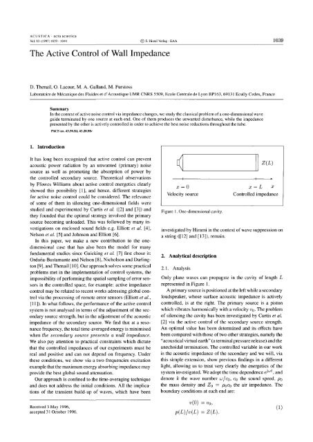
x=O<br />
Velocity source<br />
Figure I. One-dimensional cavity.<br />
investigated by Hirami in the context <strong>of</strong> wave suppression on<br />
a string ([12] and [13]), remain.<br />
2. Analytical description<br />
2.1. Analysis<br />
x = L x<br />
<strong>Control</strong>led impedance<br />
Only plane waves can propagate in the cavity <strong>of</strong> length L<br />
represented in Figure I.<br />
A primary source is positioned at the left while a secondary<br />
loudspeaker, whose surface acoustic impedance is actively<br />
controlled, is at the right. <strong>The</strong> primary source is a piston<br />
which vibrates harmonically with a velocity Vo. <strong>The</strong> problem<br />
<strong>of</strong> silencing the cavity has been investigated by Curtis et ai.<br />
[2] via the active control <strong>of</strong> the secondary source strength.<br />
An optimal value has been determined and its effects have<br />
been compared with those <strong>of</strong> two other strategies, namely the<br />
"acoustical virtual earth" (a terminal pressure release) and the<br />
anechoidal termination. <strong>The</strong> controlled variable in our work<br />
is the acoustic impedance <strong>of</strong> the secondary and we will, via<br />
this simple extension, show previous findings in a different<br />
light, allowing us to treat very clearly the energetics <strong>of</strong> the<br />
system investigated. We adopt the time dependence ejwt , and<br />
denote k the wave number w j Co, Co the sound speed, Po<br />
the mass density and Zo = Poco the air impedance. <strong>The</strong><br />
boundary conditions at each end are:<br />
V(O) = Vo,<br />
p(L)jv(L) = Z(L).<br />
(1)
1040 <strong>The</strong>nail et al.: <strong>Active</strong> control <strong>of</strong> wall impedance<br />
1.6<br />
1.2<br />
0.4<br />
a a 100 200 JOO<br />
Frequency (Hz)<br />
Figure 2. Variation <strong>of</strong> the time-averaged kinetic energy with the<br />
frequency.<br />
........,~O - - .'~O.S- ,~1 - - -,-2 - "Ofty ------- 'm'"<br />
16<br />
1.2<br />
0.4<br />
a - .:.::f.··--o<br />
100<br />
200 300<br />
Frequency (Hz)<br />
Figure 3. Variation <strong>of</strong> the time-averaged potential energy with the<br />
frequency.<br />
<strong>The</strong> reduced impedance being defined by ((X) = Z (x )/ Zo ,<br />
the acoustic pressure and velocity are:<br />
p(x) = ZOVO [(1 + ((L)) ejk(L-x)<br />
- (1- ((L)) e-jk(L-X)]<br />
x [(1 + ((L))e jkL<br />
v(x) = vo[(1 +((L)) ejk(L-x)<br />
+ (1-((L))e- jkLr1<br />
, (2)<br />
+ (1 - ((L)) e-jk(L-X)]<br />
x [(1+ ((L)) e jkL<br />
+ (1-((L))e- jkLr1<br />
. (3)<br />
<strong>The</strong>n, it is straightforward to derive the time-averaged kinetic,<br />
potential and total energies in the wave guide:<br />
poV6 [(1 + 1((L)1 2 )L + (1-1((L)12) sin2kL<br />
4 2k<br />
+ j(((L) _ (*(L)) 1- C;;2kL]<br />
400<br />
400<br />
ACUSTICA . acta acustica<br />
Vol. 83 (1997)<br />
Figure 4. Variation <strong>of</strong> the time-averaged total energy with the frequency.<br />
x [1 + 1((L)1 2 + (1-1((L)1 2 ) cos2kL<br />
+ j (((L) - (*(L)) sin2kLr1,<br />
2<br />
Ep = po;o [(1 + 1((L)1 2 )L<br />
_ (1-1((L)12) sin2kL<br />
2k<br />
_ j(((L) _ (*(L)) 1- COS2kL]<br />
2k<br />
x [1 + 1((L)1 2 + (1-1((L)12) cos2kL<br />
+ j(((L) - (*(L)) sin2kLrl,<br />
Etot = pO~6L [(1 + 1((L)1 2 )]<br />
X [1 + 1((L)1 2 + (1 - 1((L)1 2 ) cos 2kL<br />
+ j(((L) - (*(L)) sin2kLrl.<br />
Both time-averaged kinetic and potential energies tend to be<br />
equal to one half <strong>of</strong> the total energy as frequency increases.<br />
Figures 2, 3 and 4 give their respective evolutions with the<br />
frequency, for different terminal impedances. It comes out<br />
that as soon as frequency exceeds the first anti-resonance, the<br />
kinetic, potential and total energies have the same shape, for<br />
any terminal impedance value. <strong>The</strong> potential energy provides<br />
a suitable information about the evolution <strong>of</strong> the total energy<br />
we will exploit in {lur experiments, like in the referenced<br />
prior works.<br />
2.2. <strong>The</strong> optimal impedance<br />
<strong>The</strong> determination <strong>of</strong> the extrema <strong>of</strong> the time averaged total<br />
energy (expression 6) as a function <strong>of</strong> the terminal impedance<br />
is straightforward. <strong>The</strong> maxima are given by:<br />
(LMax = j cotan kL,<br />
while the minima are:<br />
(Lmin = -j tan kL.<br />
(4)<br />
(5)<br />
(6)<br />
(7)<br />
(8)
ACUSTICA . acta acustica<br />
Vol. 83 (1997)<br />
primary source<br />
input signal<br />
Va<br />
scanning<br />
microphone<br />
<strong>The</strong> latter expression (also obtained by Darlington and<br />
Avis [14]) may be deduced from the optimal strategy defined<br />
by Curtis et ai., namely v(L) = v(O) cos kL, recognizing<br />
that:<br />
where Zss is the secondary source radiation impedance,<br />
Zps is the primary to secondary transfer impedance, H =<br />
-v(L)/v(O) is the sources strength ratio.<br />
<strong>The</strong> energetics <strong>of</strong> the system terminated by the optimal<br />
impedance is examined via the impedance transfer formula:<br />
((0) = -j((L) cotan kL + 1.<br />
((L) - j cotan kL<br />
(9)<br />
(10)<br />
Thus, the terminal impedance (Lmin = -j tan kL at x = L,<br />
which leads to energy minima, is the impedance which gives<br />
((x) = 0 at x = 0 and the time-averaged acoustic intensity<br />
at the primary source is exactly zero. We have refound<br />
in a simple way that the "optimal" impedance neither supplies<br />
nor absorbs any power, while also preventing sound<br />
power radiation by the primary source. <strong>The</strong> maximally absorbent<br />
impedance (( L) = 1 presents the interesting feature<br />
<strong>of</strong> flattening the guide's acoustic response, thus reducing the<br />
potentially damaging effect <strong>of</strong> resonances, but does not allow<br />
the energy in the tube to be minimum.<br />
As seen above, the optimal impedance (Lmin is frequency<br />
dependent and the particular cases <strong>of</strong> the rigid cavity resonances<br />
and anti-resonances will now be considered. At a<br />
tube's resonance (kL = mr), the expression (8) reduces to<br />
(Lmin = 0, and the impedance approach shows clearly that a<br />
pressure release at x = L allows the best global sound attenuation<br />
in the tube. At anti-resonances (kL = (2n+ 1)7r /2), the<br />
terminating infinite impedance is the optimal boundary condition,<br />
while a null impedance causes the total time-averaged<br />
energy to be infinite. If we consider the control <strong>of</strong> any other<br />
frequency, the experimental achievement <strong>of</strong> the imaginary<br />
and frequency dependent optimal impedance (Lmin is more<br />
difficult. It is seen from Figure 4 that (( L) = 1 provides good<br />
energy reduction in the frequency region close to a resonance<br />
p(x)<br />
<strong>The</strong>nail et al.: <strong>Active</strong> control <strong>of</strong> wall impedance 1041<br />
Figure 5. Experimental set-up.<br />
but creates some amplification when the excitation frequency<br />
is close to an anti-resonance. <strong>The</strong>se relatively mediocre performances<br />
become the best which can be obtained when one<br />
resonance and one anti-resonance are simultaneously and<br />
equally excited, as will be experimented below. In addition,<br />
it is likely that this strategy, even somewhat suboptimal, is<br />
the attractive compromise to be applied in real situations<br />
including significantly broadband excitations.<br />
3. Experiments<br />
In order to illustrate some <strong>of</strong> the results presented above, we<br />
exploit a set-up previously designed for active impedance<br />
control experiments in an impedance tube [15], [9].<br />
3.1. Set-up<br />
<strong>The</strong> cavity is a O.88m long square hard-walled tube, terminated<br />
at each end by two identical loudspeakers. <strong>The</strong>y<br />
represent the velocity source, and the controlled impedance,<br />
respectively. <strong>The</strong>ir square flat membrane fills almost exactly<br />
the tube cross section (O.12mxO.12m). For the experimental<br />
frequencies, the tube is one-dimensional, even very closely<br />
to each loudspeaker. In the preceding section, the velocity<br />
<strong>of</strong> the primary source is assumed to be constant. Thus, an<br />
accelerometer <strong>of</strong> negligible mass is put on its membrane in<br />
order to balance the loudspeaker efficiency which varies with<br />
the frequency and the acoustic load presented by the cavity<br />
(preliminary experiments have taught us that this point was<br />
<strong>of</strong> great importance). <strong>The</strong> acoustic impedance at the membrane<br />
<strong>of</strong> the secondary loudspeaker is controlled via another<br />
accelerometer and a microphone. <strong>The</strong> "Filtered-X" LMS algorithm<br />
is implemented on a numerical filter whose input<br />
is the electric signal which feeds the primary source. <strong>The</strong><br />
secondary signal which is delivered at the output is amplified<br />
and connected to the secondary source. <strong>The</strong> energy <strong>of</strong> the<br />
error signal € = P - Z V is minimized, and the impedance Z<br />
is produced. <strong>The</strong> acoustic field inside the tube along its axis<br />
is scanned via a microphone, which allows also a supplementary<br />
check <strong>of</strong> the terminal impedance value via a variation
1042 <strong>The</strong>nail et al.: <strong>Active</strong> control <strong>of</strong> wall impedance<br />
......... !:zO - - . !:zO.S - !:z! -. - +2 .... !:z4 - !:mfl,<br />
20 o 0.2<br />
Figure 6. Sound pressure level variation along the tube axis near an<br />
anti-resonance at f = 291 Hz. Calculations.<br />
Figure 7. Sound pressure level variation along the tube axis near an<br />
anti-resonance at f = 291 Hz. Measurements.<br />
<strong>of</strong> Chung and Blaser's method [16], presented by Chu [17].<br />
Finally, it has been seen in the preceding section that for<br />
frequencies exceeding the first anti-resonance <strong>of</strong> 97 Hz, the<br />
time-averaged total and potential energies tend to be proportional.<br />
Consequently, the evolution <strong>of</strong> potential energy may<br />
be used to describe the total energy variations. Like in Curtis<br />
et at., we use the indicator <strong>of</strong> the sum <strong>of</strong> the mean squared<br />
sound pressures sensed along the tube axis,<br />
N<br />
Jp = 2:P;'<br />
i=l<br />
Figure 5 represents the overall experimental set-up.<br />
3.2. <strong>Control</strong> near an anti-resonance at f = 291 Hz<br />
(11)<br />
Figure 6 represents the sound pressure level inside the<br />
tube according to expression (2), for different terminal<br />
impedances, while the corresponding experimental measurements<br />
are shown in Figure 7. A good agreement is generally<br />
observed and confirms that a strictly local pressure release<br />
may involve large pressure levels everywhere else in the tube.<br />
<strong>The</strong> discrete sum <strong>of</strong> mean squared levels and the impedance<br />
measured via the Chu's method are reported in Table I.<br />
......+0 _,+o.S-!:z1 -'-+2<br />
ACUSTICA· acta acustica<br />
Vol. 83 (1997)<br />
Figure 8. Sound pressure level variation along the tube axis near a<br />
resonance at f = 388 Hz. Calculations .<br />
10<br />
-50<br />
-60 o<br />
........ !:zO - - . !:-0.5 - !:z! -. -' +2<br />
Figure 9. Sound pressure level variation along the tube axis near a<br />
resonance at f = 388 Hz. Measurements.<br />
It comes out from the figures that actual sound levels<br />
should be much higher for ((L) = O. <strong>The</strong> impedance<br />
achieved at the guide termination is not exactly zero and<br />
introduces a weak damping which is sufficient to explain the<br />
main discrepancy between measurements and results from<br />
expression (2).<br />
3.3. <strong>Control</strong> near a resonance at f = 388 Hz<br />
<strong>The</strong> expected sound pressure levels are reported in Figure 8,<br />
while the measurements and the estimated potential energy in<br />
the guide are shown in Figure 9, and in Table II, respectively.<br />
In this case, the null impedance is the impedance which<br />
allows the best global sound reduction in the tube. This result<br />
is clear: assigning an active pressure release at the end <strong>of</strong> our<br />
guide is equivalent to adding a "virtual" AI4 length, in such<br />
a way that an initially resonant frequency presents now an<br />
anti-resonant behaviour.<br />
3.4. <strong>Control</strong> <strong>of</strong> both frequencies<br />
We report here the control <strong>of</strong> a particular signal composed<br />
<strong>of</strong> one resonance and one anti-resonance equally excited.<br />
<strong>The</strong> calculated sound pressure levels are shown in Figure 10,
ACUSTICA . acta acustica<br />
Vol. 83 (1997) <strong>The</strong>nail et al.: <strong>Active</strong> control <strong>of</strong> wall impedance 1043<br />
Table I. Estimation <strong>of</strong> the potential energy in the guide excited near an anti-resonance at f = 291 Hz, for different terminal impedances.<br />
(Th 0 0.5 1 2 4 00<br />
(Mes < 0.1 + jO.1 0.6 - jO.O 1.2 + jO.1 2.1 + jO.6 3.7 + jO.8 5.6 + j7.4<br />
Jp 9.3dB -0.2dB -2.4dB -3.4 dB -3.7dB -3.8dB<br />
Table II. Estimation <strong>of</strong> the potential energy in the guide excited near a resonance at f = 388 Hz, for different terminal impedances.<br />
(Th 0 0.5 1 2 4 00<br />
(Mes < 0.1 + jO.1 0.6 - jO.1 1.3 - jO.1 2.3 + jO.2 4.6 + jO.6 0.2 + j13.4<br />
Jp -5.1dB -3.6dB -1.6 dB 1.5 dB 4.7dB 11.3 dB<br />
80<br />
70<br />
.0<br />
50<br />
....... {~O - - . {~o.S- {~1 - - +2<br />
;0 o 0.2 0.4 0.6<br />
Position (m)<br />
Figure 10. Sound pressure level variation along the tube axis. Two<br />
frequencies excitations: h = 291 Hz, h = 388 Hz. Calculations.<br />
Table III. Estimation <strong>of</strong> the potential energy in the guide, when<br />
simultaneously and equally excited at f = 291 Hz and at f =<br />
388Hz.<br />
<strong>Impedance</strong> ( 0 0.5 1 2 4 00<br />
Jp [dB] 8.6 4.0 3.9 5.3 7.3 12.47<br />
while the measurements and the estimated potential energy<br />
in the guide are reported in Figure 11 and in Table III, respectively.<br />
In the case <strong>of</strong> positive real impedances, (( L) = 1<br />
produces the best global sound attenuation.<br />
3.5. Discussion about the impedances achieved<br />
We point out first that the theoretical case <strong>of</strong> an infinite<br />
impedance has been replaced during the experiments by a<br />
zero velocity condition at the controlled loudspeaker.<br />
What mostly explains the differences between the theoretical<br />
and measured impedances (Tables I, II, and III) is<br />
that acoustic pressure and velocity are not equally delayed<br />
by their respective measurement devices before being converted<br />
in digital signals updating the controller's coefficients.<br />
......... {~O - - . {~o.S- {~1 -. - +2 ..... H - ~Of\y(~O)<br />
10<br />
-10<br />
-20<br />
-30<br />
-40 o<br />
Figure 11. Sound pressure level variation along the tube axis. Two<br />
frequencies excitations: h = 291 Hz, h = 388 Hz. Measurements.<br />
<strong>The</strong> problem <strong>of</strong> transduction errors in the case <strong>of</strong> the active<br />
anechoic termination has been investigated by Darlington et<br />
at. [18], and it may be added to the experimental difficulties<br />
reviewed in the latter reference (transduction and digital<br />
signal processing errors), that the impedance measurement<br />
accuracy is also strongly dependent on the desired terminal<br />
impedance. In particular, very high and low impedances<br />
for which the acoustic field in the guide is very reactive,<br />
are more subjected to measurement errors than an absorbing<br />
termination.<br />
Finally, the achievement <strong>of</strong> a given real impedance over<br />
wide frequency ranges has also been attempted. <strong>The</strong> attenuation<br />
at each frequency was not significantly different from<br />
the attenuation achieved using a single frequency primary<br />
signal. However, it clearly confirms from a practical point <strong>of</strong><br />
view the usefullness <strong>of</strong> using, as active impedance, a porous<br />
layer backed by an active acoustical short-circuit, as experimented<br />
first by Guicking and Lorentz [19], then by <strong>The</strong>nail<br />
et at. [20].
1044 <strong>The</strong>nail et al.: <strong>Active</strong> control <strong>of</strong> wall impedance<br />
4. Conclusion<br />
We have demonstrated, via the acoustics <strong>of</strong> a onedimensional<br />
wave guide, the potentialities <strong>of</strong> active<br />
impedance control in silencing a system. On the one hand,<br />
this approach gives clear teachings and completes previous<br />
contributions by other authors about the energetics <strong>of</strong> active<br />
control. On the other hand, the given example demonstrates<br />
that impedance control gives the same optimal performance<br />
as classical feedforward schemes.<br />
In our wave guide, the optimal terminal impedance which<br />
minimizes the total energy by preventing power radiation by<br />
the primary source, has been experienced near a resonance<br />
where the optimal impedance becomes an active pressure<br />
release. This work must now account for significantly broadband<br />
and unexpected disturbances and will probably show<br />
an increasing importance to the design <strong>of</strong> active absorbers.<br />
Acknowledgement<br />
<strong>The</strong> authors express their gratitude to Pr<strong>of</strong>essor J. E. Ffowcs<br />
Williams (University <strong>of</strong> Cambridge, U. K.) for many comments<br />
and discussions. D. <strong>The</strong>nail is currently post-doctoral<br />
fellow <strong>of</strong> the <strong>Centre</strong> National d'Etudes Spatiales.<br />
References<br />
[1] J. E. Ffowcs Williams: Anti-sound. Proc. R. Soc. London 395<br />
(1984) 63-88. Ser. A.<br />
[2] A. R. D. Curtis, P. A. Nelson, S. J. Elliott, A. J. Bullmore:<br />
<strong>Active</strong> suppression <strong>of</strong> acoustic resonance. J. Acous. Soc. Am.<br />
81 (1987) 624-631.<br />
[3] A. R. D. Curtis, P. A. Nelson, S. J. Elliott: <strong>Active</strong> reduction<br />
<strong>of</strong> a one-dimensional enclosed sound field: An experimental<br />
investigation <strong>of</strong> three control strategies. J. Acous. Soc. Am. 88<br />
(1990) 2265-2268.<br />
[4] S. J. Elliott, P. Joseph, P. A. Nelson, M. E. Johnson: Power<br />
output minimization and power absorption in the active control<br />
<strong>of</strong> sound. J. Acous. Soc. Am. 90 (1991) 2501-2511.<br />
ACUSTlCA· acta acustica<br />
Vol. 83 (1997)<br />
[5] P. A. Nelson, J. K. Hammond, P. Joseph, S. J. Elliott: <strong>Active</strong><br />
control <strong>of</strong> stationary random sound fields. J. Acous. Soc. Am.<br />
87 (1990) 963-975.<br />
[6] M. E. Johnson, S. J. Elliott: Measurement <strong>of</strong> acoustic power<br />
output in the active control <strong>of</strong> sound. J. Acous. Soc. Am. 93<br />
(1993) 1453-1459.<br />
[7] D. Guicking, K. Karcher, M. A. Rollwage: Coherent active<br />
methods for applications in room acoustics. J. Acous. Soc.<br />
Am. 78 (1985) 1426-1434.<br />
[8] F. Ordufia Bustamante, P. A. Nelson: An adaptive controller for<br />
the active absorption <strong>of</strong> sound. J. Acous. Soc. Am. 91 (1992)<br />
2740-2747.<br />
[9] G. C. Nicholson, P. Darlington: <strong>Active</strong> control <strong>of</strong> acoustic absorption,<br />
reflection and transmission. Proc. LO.A., 1993. 403-<br />
409.<br />
[10] D. <strong>The</strong>nail: Contr61e actif d' impedance et optimisation des performances<br />
d'un materiau poreux. Dissertation. Ecole Centrale<br />
de Lyon, 1995. 95-11.<br />
[11] S. J. Elliott, T. J. Sutton, B. Rafaely, M. Johnson: Design <strong>of</strong><br />
feedback controllers using a feedforward approach. Proc. <strong>Active</strong><br />
95, Newport Beach, CA, USA, 1995. 863-874.<br />
[12] N. Hirami: Is the optimal damper a good attenuator? Proc.<br />
Idee-Force EUR' ACOUSTICS, Ecole Centrale de Lyon, 1992.<br />
W14.<br />
[13] N. Hirami: Optimal energy absorption for wave suppression.<br />
13eme colloque d' Aero et Hydroacoustique, Ecole Centrale de<br />
Lyon, 1993. 41-45.<br />
[14] P. Darlington, M. R. Avis: Modifying low frequency room<br />
acoustics 2: global control using active absorbers. Proc. LO.A.,<br />
1995. 87-96.<br />
[15] D. <strong>The</strong>nail, M. A. Galland: Development <strong>of</strong> an active anechoidal<br />
boundary. Proc. Idee-Force EUR' ACOUSTICS, Ecole<br />
Centrale de Lyon, 1992. W4.<br />
[16] J. Y. Chung, D. A. Blaser: Transfer function method <strong>of</strong> measuring<br />
in-duct acoustic properties. J. Acous. Soc. Am. 68 (1980)<br />
907-922.<br />
[17] W. T. Chu: Transfer function technique for impedance and<br />
absorption measurements in an impedance tube using a single<br />
microphone. J. Acous. Soc. Am. 80 (1986) 555-560.<br />
[18] P. Darlington, G. C. Nicholson, S. E. Mercy: Inputtransduction<br />
errors in active acoustic absorbers. Acta Acustica 3 (1995)<br />
345-349.<br />
[19] D. Guicking, E. Lorentz: An active sound absorber with porous<br />
plate. ASME J. Vib. Acoustics, Stress Reliab. Des. 106 (1984)<br />
389--404.<br />
[20] D. <strong>The</strong>nail, M. A. Galland, M. Furstoss, M. Sunyach: Absorption<br />
by an actively enhanced material. Proc. <strong>of</strong> the 1994 ASME<br />
Winter Annual Meeting, Chicago, II, USA, 1994. 441--448.<br />
AM-I6D.