The Active Control of Wall Impedance - Centre Acoustique

More documents

Recommendations

Info

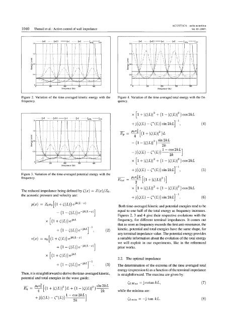
1040 Thenail et al.: Active control of wall impedance 1.6 1.2 0.4 a a 100 200 JOO Frequency (Hz) Figure 2. Variation of the time-averaged kinetic energy with the frequency. ........,~O - - .'~O.S- ,~1 - - -,-2 - "Ofty ------- 'm'" 16 1.2 0.4 a - .:.::f.··--o 100 200 300 Frequency (Hz) Figure 3. Variation of the time-averaged potential energy with the frequency. The reduced impedance being defined by ((X) = Z (x )/ Zo , the acoustic pressure and velocity are: p(x) = ZOVO [(1 + ((L)) ejk(L-x) - (1- ((L)) e-jk(L-X)] x [(1 + ((L))e jkL v(x) = vo[(1 +((L)) ejk(L-x) + (1-((L))e- jkLr1 , (2) + (1 - ((L)) e-jk(L-X)] x [(1+ ((L)) e jkL + (1-((L))e- jkLr1 . (3) Then, it is straightforward to derive the time-averaged kinetic, potential and total energies in the wave guide: poV6 [(1 + 1((L)1 2 )L + (1-1((L)12) sin2kL 4 2k + j(((L) _ (*(L)) 1- C;;2kL] 400 400 ACUSTICA . acta acustica Vol. 83 (1997) Figure 4. Variation of the time-averaged total energy with the frequency. x [1 + 1((L)1 2 + (1-1((L)1 2 ) cos2kL + j (((L) - (*(L)) sin2kLr1, 2 Ep = po;o [(1 + 1((L)1 2 )L _ (1-1((L)12) sin2kL 2k _ j(((L) _ (*(L)) 1- COS2kL] 2k x [1 + 1((L)1 2 + (1-1((L)12) cos2kL + j(((L) - (*(L)) sin2kLrl, Etot = pO~6L [(1 + 1((L)1 2 )] X [1 + 1((L)1 2 + (1 - 1((L)1 2 ) cos 2kL + j(((L) - (*(L)) sin2kLrl. Both time-averaged kinetic and potential energies tend to be equal to one half of the total energy as frequency increases. Figures 2, 3 and 4 give their respective evolutions with the frequency, for different terminal impedances. It comes out that as soon as frequency exceeds the first anti-resonance, the kinetic, potential and total energies have the same shape, for any terminal impedance value. The potential energy provides a suitable information about the evolution of the total energy we will exploit in {lur experiments, like in the referenced prior works. 2.2. The optimal impedance The determination of the extrema of the time averaged total energy (expression 6) as a function of the terminal impedance is straightforward. The maxima are given by: (LMax = j cotan kL, while the minima are: (Lmin = -j tan kL. (4) (5) (6) (7) (8)
ACUSTICA . acta acustica Vol. 83 (1997) primary source input signal Va scanning microphone The latter expression (also obtained by Darlington and Avis [14]) may be deduced from the optimal strategy defined by Curtis et ai., namely v(L) = v(O) cos kL, recognizing that: where Zss is the secondary source radiation impedance, Zps is the primary to secondary transfer impedance, H = -v(L)/v(O) is the sources strength ratio. The energetics of the system terminated by the optimal impedance is examined via the impedance transfer formula: ((0) = -j((L) cotan kL + 1. ((L) - j cotan kL (9) (10) Thus, the terminal impedance (Lmin = -j tan kL at x = L, which leads to energy minima, is the impedance which gives ((x) = 0 at x = 0 and the time-averaged acoustic intensity at the primary source is exactly zero. We have refound in a simple way that the "optimal" impedance neither supplies nor absorbs any power, while also preventing sound power radiation by the primary source. The maximally absorbent impedance (( L) = 1 presents the interesting feature of flattening the guide's acoustic response, thus reducing the potentially damaging effect of resonances, but does not allow the energy in the tube to be minimum. As seen above, the optimal impedance (Lmin is frequency dependent and the particular cases of the rigid cavity resonances and anti-resonances will now be considered. At a tube's resonance (kL = mr), the expression (8) reduces to (Lmin = 0, and the impedance approach shows clearly that a pressure release at x = L allows the best global sound attenuation in the tube. At anti-resonances (kL = (2n+ 1)7r /2), the terminating infinite impedance is the optimal boundary condition, while a null impedance causes the total time-averaged energy to be infinite. If we consider the control of any other frequency, the experimental achievement of the imaginary and frequency dependent optimal impedance (Lmin is more difficult. It is seen from Figure 4 that (( L) = 1 provides good energy reduction in the frequency region close to a resonance p(x) Thenail et al.: Active control of wall impedance 1041 Figure 5. Experimental set-up. but creates some amplification when the excitation frequency is close to an anti-resonance. These relatively mediocre performances become the best which can be obtained when one resonance and one anti-resonance are simultaneously and equally excited, as will be experimented below. In addition, it is likely that this strategy, even somewhat suboptimal, is the attractive compromise to be applied in real situations including significantly broadband excitations. 3. Experiments In order to illustrate some of the results presented above, we exploit a set-up previously designed for active impedance control experiments in an impedance tube [15], [9]. 3.1. Set-up The cavity is a O.88m long square hard-walled tube, terminated at each end by two identical loudspeakers. They represent the velocity source, and the controlled impedance, respectively. Their square flat membrane fills almost exactly the tube cross section (O.12mxO.12m). For the experimental frequencies, the tube is one-dimensional, even very closely to each loudspeaker. In the preceding section, the velocity of the primary source is assumed to be constant. Thus, an accelerometer of negligible mass is put on its membrane in order to balance the loudspeaker efficiency which varies with the frequency and the acoustic load presented by the cavity (preliminary experiments have taught us that this point was of great importance). The acoustic impedance at the membrane of the secondary loudspeaker is controlled via another accelerometer and a microphone. The "Filtered-X" LMS algorithm is implemented on a numerical filter whose input is the electric signal which feeds the primary source. The secondary signal which is delivered at the output is amplified and connected to the secondary source. The energy of the error signal € = P - Z V is minimized, and the impedance Z is produced. The acoustic field inside the tube along its axis is scanned via a microphone, which allows also a supplementary check of the terminal impedance value via a variation
Page 1: ACUSTICA· acta acustica Vol. 83 (1
Page 5 and 6: ACUSTICA . acta acustica Vol. 83 (1

The Active Control of Wall Impedance - Centre Acoustique

You also want an ePaper? Increase the reach of your titles

Delete template?

Save as template?