The Active Control of Wall Impedance - Centre Acoustique
The Active Control of Wall Impedance - Centre Acoustique
The Active Control of Wall Impedance - Centre Acoustique

You also want an ePaper? Increase the reach of your titles
YUMPU automatically turns print PDFs into web optimized ePapers that Google loves.
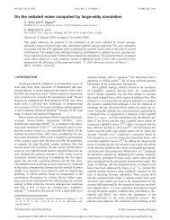
1042 <strong>The</strong>nail et al.: <strong>Active</strong> control <strong>of</strong> wall impedance<br />
......... !:zO - - . !:zO.S - !:z! -. - +2 .... !:z4 - !:mfl,<br />
20 o 0.2<br />
Figure 6. Sound pressure level variation along the tube axis near an<br />
anti-resonance at f = 291 Hz. Calculations.<br />
Figure 7. Sound pressure level variation along the tube axis near an<br />
anti-resonance at f = 291 Hz. Measurements.<br />
<strong>of</strong> Chung and Blaser's method [16], presented by Chu [17].<br />
Finally, it has been seen in the preceding section that for<br />
frequencies exceeding the first anti-resonance <strong>of</strong> 97 Hz, the<br />
time-averaged total and potential energies tend to be proportional.<br />
Consequently, the evolution <strong>of</strong> potential energy may<br />
be used to describe the total energy variations. Like in Curtis<br />
et at., we use the indicator <strong>of</strong> the sum <strong>of</strong> the mean squared<br />
sound pressures sensed along the tube axis,<br />
N<br />
Jp = 2:P;'<br />
i=l<br />
Figure 5 represents the overall experimental set-up.<br />
3.2. <strong>Control</strong> near an anti-resonance at f = 291 Hz<br />
(11)<br />
Figure 6 represents the sound pressure level inside the<br />
tube according to expression (2), for different terminal<br />
impedances, while the corresponding experimental measurements<br />
are shown in Figure 7. A good agreement is generally<br />
observed and confirms that a strictly local pressure release<br />
may involve large pressure levels everywhere else in the tube.<br />
<strong>The</strong> discrete sum <strong>of</strong> mean squared levels and the impedance<br />
measured via the Chu's method are reported in Table I.<br />
......+0 _,+o.S-!:z1 -'-+2<br />
ACUSTICA· acta acustica<br />
Vol. 83 (1997)<br />
Figure 8. Sound pressure level variation along the tube axis near a<br />
resonance at f = 388 Hz. Calculations .<br />
10<br />
-50<br />
-60 o<br />
........ !:zO - - . !:-0.5 - !:z! -. -' +2<br />
Figure 9. Sound pressure level variation along the tube axis near a<br />
resonance at f = 388 Hz. Measurements.<br />
It comes out from the figures that actual sound levels<br />
should be much higher for ((L) = O. <strong>The</strong> impedance<br />
achieved at the guide termination is not exactly zero and<br />
introduces a weak damping which is sufficient to explain the<br />
main discrepancy between measurements and results from<br />
expression (2).<br />
3.3. <strong>Control</strong> near a resonance at f = 388 Hz<br />
<strong>The</strong> expected sound pressure levels are reported in Figure 8,<br />
while the measurements and the estimated potential energy in<br />
the guide are shown in Figure 9, and in Table II, respectively.<br />
In this case, the null impedance is the impedance which<br />
allows the best global sound reduction in the tube. This result<br />
is clear: assigning an active pressure release at the end <strong>of</strong> our<br />
guide is equivalent to adding a "virtual" AI4 length, in such<br />
a way that an initially resonant frequency presents now an<br />
anti-resonant behaviour.<br />
3.4. <strong>Control</strong> <strong>of</strong> both frequencies<br />
We report here the control <strong>of</strong> a particular signal composed<br />
<strong>of</strong> one resonance and one anti-resonance equally excited.<br />
<strong>The</strong> calculated sound pressure levels are shown in Figure 10,