IRIS RECOGNITION BASED ON HILBERT–HUANG TRANSFORM 1 ...

ROI {
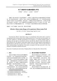
Iris Recognition Based on Hilbert–Huang Transform 629
Fig. 3. The normalized iris image is vertically divided into four subregions. The three subregions
1,2and3aretheROI.
210
200
190
180
170
160
150
140
130
120
0 50 100 150 200 250 300 350 400 450 500
x
1
2
3
4
200
150
100
0
50
0
50 100 150 200 250 300 350 400 450 500
−50
0
50
50 100 150 200 250 300 350 400 450 500
c1
c2
c3
c4
c5
r
0
−50
0
50
50 100 150 200 250 300 350 400 450 500
0
−50
0
50
50 100 150 200 250 300 350 400 450 500
0
−50
0 50 100 150 200 250 300 350 400 450 500
20
0
−20
0
200
50 100 150 200 250 300 350 400 450 500
150
0 50 100 150 200 250 300 350 400 450 500
Fig. 4. Left, the 11th line signal of the normalized iris image in Fig. 3 along the horizontal
direction. Right, the EMD decomposition result of the 11th line signal.
An iris consists of some basic elements which are similar each other and interlaced
each other. Hence, an iris image is generally periodic to some extent along
some directions, that is, some approximate periods are embed in the iris image. As
an example, let us observe the 11th line signal of the normalized iris image in Fig. 3
along the horizontal direction, as show in the left of Fig. 4. It can be seen that most
of the durations of the waves are similar, i.e. some main frequencies embed in the
signal. As we know, the EMD can extract the low-frequency oscillations very well. 11
With EMD, the decomposition result of the 11th line signal is shown in the right of
Fig. 4. It can be seen that two main approximate periods are extracted in the third
and fourth IMFs. To show it clearly, we plot the original signal (solid line) and the
third IMF (dash line) together in the interval [320, 450] in the left of Fig. 5. It can
be seen that this IMF characterizes the proximate period of the waveform quite well
and the period is about 15 (i.e. the frequency is about 1/15 ≈ 0.067). Similarly, we
plot the original signal (solid line) and the fourth IMF (dash line) together in the
interval [320, 450] in the right of Fig. 5. It can be seen that this IMF characterizes
the proximate period and the variety of the amplitude. This period is about 26 (i.e.
the frequency is about 1/26 ≈ 0.0385).
According to Eq. (3), we can compute the Hilbert marginal spectrum of the
11th line signal of the normalized iris image in Fig. 3, as shown in the left of
Fig. 6. It is evident that the two main frequencies can be extracted from the Hilbert
marginal spectrum correctly. Based on lots of experiments and analysis we found