EE 591 K. Nayak MR Imaging and Reconstruction Homework #4 ...

EE 591 K. Nayak
MR Imaging and Reconstruction
Homework #4
Due: Monday, January 27th (in class)
• This homework assignment depends heavily on Matlab. You will write simple image
reconstruction scripts and a simple Bloch simulator, and then simulate excitation
pulses as well as some off-resonance artifacts.
• You may work on the homework in groups, but must each submit independently and
provide your own explanations of the images. If you are not an experienced Matlab
user, please work with someone who is.
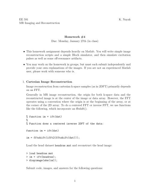
1. Cartesian Image Reconstruction
Image reconstruction from cartesian k-space samples (as in 2DFT) primarily depends
on an FFT.
Generally in MR image reconstruction, the origin for both k-space data and the
reconstructed image is at the center of the image or data array. However, the FFT
operates using a convention where the origin is at the beginning of the array, or at
the corner of the 2D array. To do a centered FFT or inverse FFT, we use functions
like the following, which incorporate an fftshift().
% function im = ift(dat)
%
% Function does a centered inverse 2DFT of the data:
function im = ift(dat)
im = fftshift(ifft2(fftshift(dat)));
Load the head dataset headraw.mat and reconstruct the head image:
> load headraw.mat
> im = ift(headraw);
> dispimage(abs(im));
Submit code, images, and answers for the following questions:
1

(a) Upsample the original raw data matrix to 512x512 by inserting lines of zeros
in between the data samples (in both directions). What happens to the reconstructed
image? Anything useful?
(b) Zero-pad the original raw data matrix up to 512x512 and reconstruct. What
happens to the reconstructed image? Anything useful?
2. Test Objects
When simulating sequences it’s often useful to fabricate data for hypothetical objects.
An easy way to do this is to design a test object that is made up of shapes with
continuous Fourier transforms that are easy to describe analytically.
For example, a circular object rect(r) would have a continuous fourier transform
that is jinc(kr), and rect(x)rect(y) has a continuous fourier transform that is
sinc(kx)sinc(ky).
Use the following commands to generate one possible test object:
> krange = (-128:127)/256;
> [ky kx] = meshgrid(krange,krange);
> kr = sqrt(kx.^2 + ky.^2);
> tx_circ = 25*25*jinc(25*kr); % FTx of circle with diameter 25
> tx_rect = 5*30*sinc(5*kx).*sinc(30*ky); % FTx of rectangle 5x30
> tx = tx_circ .* exp(-j*2*pi*kx*30) ...
> + tx_rect .* exp(-j*2*pi*(-10*kx + 20*ky));
> im = ift(tx);
> figure;
> dispimage(abs(tx));
> figure;
> dispimage(abs(im));
(a) Examine the reconstructed object carefully (zoom into different areas, and window
the image). Describe artifacts that you find, and why they are there.
(b) Generate a raw data matrix for your own test object. You may use the provided
rectangle fourier() and ellipse fourier() functions. Be creative,
and make sure the test objects use up a large portion of the field of view, and
that they contain some elements that have high spatial resolution.
(c) When we simulate an object containing different tissues, it is beneficial to create
raw data matrices for each tissue type. For example:
> tx_water = 100*100*jinc(100*kr) - 50*50*jinc(50*kr);
> tx_fat = 1.2 * (50*50*jinc(50*kr));
> tx = tx_water + tx_fat;
> im = ift(tx);
> dispimage(abs(im));
2

This test image is a circle of fat surrounded by a circle of water. Note that we
made fat 20% brighter than the water.
With separated raw-data for the fat and water, it’s easier to simulate the effects
of off-resonance (or other tissue differences). In 2DFT imaging, the signal phase
due to off-resonance can be expressed as a function of kx. Suppose that the slice
is excited at t = 0, and readouts occur from t = 10 to 30 ms. Express t as a
function of kx (Note that the kx matrix values go from -0.5 to 0.5). Suppose
we are imaging at 3 Tesla so that ∆f = -440 Hz for fat. Apply the appropriate
phase to the fat raw data, and reconstruct the fat and water image. What do
you see?
You just reconstructed the image for a 20 ms readout with a 20 ms TE. Repeat
the reconstruction for a 22 ms TE, 24 ms TE, and 28 ms TE. Do you notice any
changes in the region of overlap? What is happening? Hint: look at the image
phase dispimage(angle(im)).
Now reconstruct the image for a 8 ms readout with a 20 ms TE. What do you
see?
(d) In PR and spiral imaging, the time map is a function primarily of kr. Suppose
that we are using single-sided PR sequence with readouts again occur from
t = 10 to 30 ms (this time TE = 10 ms). If t is a linear function of kr, reconstruct
the resulting image. Remember to zero-out portions of the raw data matrix
which are outside the circular region that is acquired (i.e. where kr > 0.5).
Repeat the reconstructions if the readouts are shortened to 10 ms? and again
shortened to 4 ms? (always starting 10 ms after the excitation)
Explain your findings.
3. Bloch Simulation
In this problem you will implement a Bloch equation simulator, and use it to test the
performance of excitation pulses.
In the presence of RF pulses, Gradient fields, and relaxation, the Bloch equation
dictates the behavior of spin magnetization. In the rotating frame, the magnetization
vector experiences excitation, precession, and relaxation. In reality these three things
are happening simultaneously, but a good approximation is to look at short time
intervals (dt) and simulate the effects of the three separately.
If including relaxation, off-resonance, precession due to gradients, and excitation, you
might use code similar to the following:
> Mo = 1;
> M = [0;0;Mo]; % equilibrium magnetization
...
> E1 = exp(-dt/T1);
> E2 = exp(-dt/T2);
> A = [E2 0 0; 0 E2 0; 0 0 E1];
> b = [0;0;(1-E1)];
3

...
> M = xrot(gamma*B1*dt) *M; % excitation_x: rotation about the x axis
> M = zrot(2*pi*df*dt) *M; % precession due to off-resonance (df)
> M = zrot(gamma*(Gx*x+Gy*y+Gz*z)*dt) *M;
% precession due to Gradients
> M = A*M+b*Mo; % relaxation
In this problem, you will be simulating excitation pulses, off-resonance, and gradients.
Relaxation is ignored.
Browse the provided simpulse.m file and verify that it simulates the rotations experienced
by a spin at position z due to a given b1 (RF pulse in Gauss), gz (Z gradient
in Gauss/cm), and df (off-resonant frequency in Hz).
For the following two parts assume that magnetization begins at equilibrium, that
Mo = 1, and ignore relaxation. The waveforms you will load have a sampling rate of
4µs. And gamma is 26752 rad/s/G.
(a) Load the slice selective RF pulse sliceselect.mat which contains an RF pulse
and associated Z-gradient. Simulate the excitation profile for spins with zpositions
from -1 cm to 1 cm in 0.2 mm (or smaller) increments. Plot Mx,
My, and Mz as a function of z position.
Repeat the simulation assuming off-resonance with ∆f = -440 Hz (fat). What
happens to the slice profile? What are the implications if we use this excitation
pulse to image a slice in the body that contains both water and fat?
(b) Load the spectral-spatial RF pulse specspat.mat which also contains an RF
pulse and associated Z-gradient. This is an interesting pulse design that excites
a limited range of frequencies.
Plot Mx, My, and Mz as a function of z position (for ∆f = 0).
Plot Mz, My, and Mz as a function of off-resonance (for z = 0). Let ∆f range
from -1 kHz to 1 kHz in 25 Hz increments.
OPTIONAL PART (if time permits): Make an image of the resulting transverse
magnetization (|Mr| = |Mx + iMy|), for locations ranging from z = -1 cm to
1 cm, and ∆f ranging from -1 kHz to 1 kHz in 25 Hz increments.
(c) Modify simpulse.m to incorporate relaxation. Assume T1 = 100 ms. Consider
the slice selective pulse in part (a) and determine how small T2 needs to be
before it noticeably affects the excitation profile.
Explain the slice profile changes that you notice.
4