Chapter 3 Time-to-live Covert Channels - CAIA
Chapter 3 Time-to-live Covert Channels - CAIA
Chapter 3 Time-to-live Covert Channels - CAIA

Create successful ePaper yourself
Turn your PDF publications into a flip-book with our unique Google optimized e-Paper software.
<strong>Chapter</strong> 3<br />
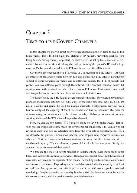
CHAPTER 3. TIME-TO-LIVE COVERT CHANNELS<br />
<strong>Time</strong>-<strong>to</strong>-<strong>live</strong> <strong>Covert</strong> <strong>Channels</strong><br />
In this chapter we analyse direct noisy s<strong>to</strong>rage channels in the IP <strong>Time</strong>-<strong>to</strong>-<strong>live</strong> (TTL)<br />
header field. The TTL field limits the lifetime of IP packets, preventing packets from<br />
living forever during routing loops [89]. A packet’s TTL is set by the sender and decre-<br />
mented by each network node along the path processing the packet’s IP header (e.g.<br />
routers). Packets are discarded if their TTL reaches zero while still in transit.<br />
<strong>Covert</strong> bits are encoded in<strong>to</strong> a TTL value, or a succession of TTL values. Although<br />
assumed <strong>to</strong> be reasonably stable between two end-points, the TTL value is nonetheless<br />
subject so some variation, as routers and middleboxes modify the TTL of packets and<br />
packets can take different paths through the network. This ‘normal’ variation causes bit<br />
substitutions on the channel; we also refer <strong>to</strong> this as TTL noise. Furthermore, reordered<br />
and lost packets may cause further bit substitutions and bit deletions.<br />
The idea of using the TTL field as covert channel is not new. However, the previously<br />
proposed modulation schemes [95, 61], ways of encoding data in<strong>to</strong> the TTL field, are<br />
not all stealthy and cannot be used for passive channels. Furthermore, previous work<br />
has not analysed the capacity of the TTL channel and has not addressed the problem<br />
of transmitting information across the channel reliably. Unlike previous work we also<br />
consider the use of the TTL channel as passive channel.<br />
First, we analyse the normal TTL variation based on several traffic traces. The re-<br />
sults provide insights in<strong>to</strong> how much the covert channel can modify TTL values without<br />
revealing itself and give an indication how large the error rate is expected <strong>to</strong> be. Then<br />
we describe the previous modulation schemes and propose new improved modulation<br />
schemes. Next, we propose an information-theoretic model for the channel and derive<br />
the channel capacity. Then we develop a pro<strong>to</strong>col for reliable data transport. Finally, we<br />
evaluate the performance of the channel.<br />
We emulate the use of different modulation schemes using overt traffic from traffic<br />
traces and measure the resulting error rates. Based on the channel model and the measured<br />
error rates we compute the capacity of the channel depending on the modulation schemes<br />
and network conditions. Depending on the available overt traffic the capacity is at least<br />
several tens, but up <strong>to</strong> over one kilobit per second even with modest packet loss and<br />
reordering. Despite the noise the capacity is substantial. Furthermore, the noise masks<br />
the covert channel, which would otherwise be trivial <strong>to</strong> detect.<br />
38
CHAPTER 3. TIME-TO-LIVE COVERT CHANNELS<br />
Table 3.1: Packet traces used in the analysis<br />
Trace Capture location Date Public<br />
<strong>CAIA</strong> Public game server at Swinburne University,<br />
Melbourne, Australia<br />
Grangenet Public game server connected <strong>to</strong> Grangenet,<br />
Canberra, Australia<br />
05/2005 – 06/2006 no<br />
05/2005 – 06/2006 no<br />
Twente Uplink of ADSL access network [165] 07/02/2004 – 12/02/2004 yes<br />
Leipzig Access router at Leipzig University [166] 21/02/2003 yes<br />
Bell Firewall at Bell Labs [166] 19/05/2002 – 20/05/2002 yes<br />
Waika<strong>to</strong> Access router at University of Waika<strong>to</strong>, New<br />
Zealand<br />
04/05/2005 no<br />
We evaluate the throughput of the developed reliable transport technique for aggregate<br />
overt traffic taken from traces under different simulated network conditions. We also<br />
analyse the throughput across a real network with different rates of TTL errors, overt<br />
packet loss and reordering, using single overt traffic flows as carrier. Comparison of the<br />
results with the channel capacity shows that our technique is not optimal, but it provides<br />
throughputs of at least 50% of the capacity, except in the case of high reordering. The<br />
throughput is up <strong>to</strong> over hundred bits per second.<br />
3.1 Normal TTL variation<br />
First we analyse ‘normal’ TTL variation (TTL noise). We analyse how TTL varies at<br />
small time scales of subsequent packets of traffic flows (series of packets with the same<br />
IP addresses, ports, and pro<strong>to</strong>col) and not only focus on variation caused by path changes<br />
as previous work [161, 162, 163, 164]. An extended version of this study is in [9].<br />
3.1.1 Datasets and methodology<br />
We use packet traces of different size, origin and date for our analysis (see Table 3.1). The<br />
<strong>CAIA</strong> trace contains only game traffic arriving at a public game server, the Grangenet<br />
trace contains game and web traffic arriving at a specific server, and the other traces<br />
contain a mix of bidirectional traffic.<br />
Usually analysis of network traffic is based on packet flows. Because we found the<br />
number of TTL changes is correlated with the number of packets and the duration of<br />
flows, we analyse many characteristics of TTL changes based on packet pairs, defined<br />
as two subsequent packets of a flow. This isolates the characteristic under study (e.g.<br />
estimated hop count) from correlated flow properties (e.g. size and duration). However,<br />
for analysis requiring a sequence of packets we still use flows (e.g. in Section 3.1.4).<br />
39
CHAPTER 3. TIME-TO-LIVE COVERT CHANNELS<br />
Table 3.2: Flows and packet pairs with/without TTL changes and percentage of changes<br />
Flows Packet pairs<br />
No change<br />
(kilo)<br />
Change<br />
(kilo)<br />
Change<br />
(%)<br />
No change<br />
(Mega)<br />
Change<br />
(kilo)<br />
Change<br />
(%)<br />
<strong>CAIA</strong> 128.6 2.8 2.1 1 456.3 340.0 0.02<br />
Grangenet 283.0 8.6 2.9 215.7 62.1 0.03<br />
Twente 1 354.6 24.7 1.8 95.5 74.8 0.08<br />
Waika<strong>to</strong> 1 255.9 57.8 4.4 21.2 86.4 0.4<br />
Bell 899.8 52.9 5.6 36.4 87.1 0.2<br />
Leipzig 7 155.1 429.1 5.7 365.5 1 822.7 0.5<br />
First, packets were grouped in<strong>to</strong> unidirectional flows according <strong>to</strong> IP addresses, port<br />
numbers and pro<strong>to</strong>col (each being a series of packet pairs). We only considered flows<br />
with at least four packets (‘minimum’ TCP flow) and an average packet rate of at least<br />
one packet per second. We extracted the series of TTL values from the IP headers. If<br />
different TTL values occur in a flow or between packet pairs this is referred <strong>to</strong> as TTL<br />
change. Otherwise we refer <strong>to</strong> the TTL being constant.<br />
3.1.2 Amount of TTL variation<br />
Table 3.2 shows the number and the percentage of flows and packet pairs with and without<br />
TTL changes (numbers are rounded). Overall, the TTL is constant for the majority of<br />
flows, but 2–6% of flows do experience TTL changes. The percentage of packet pairs<br />
with TTL changes is between 0.02–0.5%. This shows that if there is TTL variation in<br />
flows, changes occur only for a very small number of the flows’ packet pairs.<br />
3.1.3 Distinct values and change amplitudes<br />
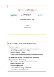
Figure 3.1 shows the cumulative density functions (CDFs) of the number of distinct TTL<br />
values per flow. Most flows with TTL variation have only two distinct TTL values. Only<br />
less than 10% of the flows have more than two values and flows with more than five<br />
different TTLs are very rare, except in the <strong>CAIA</strong> trace.<br />
We examined CDFs of the amplitude of TTL changes of packet pairs, where the am-<br />
plitude is defined as the difference between the maximum and the minimum TTL value.<br />
The amplitude is one for many packet pairs, but in some traces large numbers of packet<br />
pairs have amplitudes around 64, 127, or 191 [9]. The reason for these high amplitudes is<br />
middleboxes, such as firewalls or proxies, (re)sending packets part of the TCP handshake<br />
or teardown on behalf of end hosts (e.g. for SYN flood attack protection).<br />
The TTLs in these packets are set <strong>to</strong> the initial TTL of the middlebox, which can<br />
differ from the initial TTL used by the host. Different operating systems use different<br />
40
Proportion ≤≤ x<br />
1.00<br />
0.95<br />
0.90<br />
0.85<br />
CHAPTER 3. TIME-TO-LIVE COVERT CHANNELS<br />
0 10 20 30 40 50 60<br />
Number of distinct TTLs<br />
<strong>CAIA</strong><br />
GrangeNet<br />
Twente<br />
Waika<strong>to</strong><br />
Bell<br />
Leipzig<br />
Figure 3.1: Distribution of the number of distinct TTL values per flow<br />
Proportion ≤ x<br />
1.00<br />
0.95<br />
0.90<br />
0.85<br />
0.80<br />
<strong>CAIA</strong><br />
GrangeNet<br />
Twente<br />
Waika<strong>to</strong><br />
Bell<br />
Leipzig<br />
0 10 20 30 40 50<br />
Amplitude of estimated hop count change<br />
Figure 3.2: Distribution of the estimated hop count amplitude of packet pairs<br />
initial TTLs, the most common being: 64 (Linux, FreeBSD), 128 (Windows), 255 (Cisco)<br />
[167, 168]. Therefore, the difference of two TTLs is 64, 127, or 191 plus/minus the<br />
number of hops between middlebox and host. Because of this effect TTL changes are<br />
more likely at the start or end of TCP flows.<br />
Figure 3.2 shows the CDFs of the amplitude of the estimated hop counts of packet<br />
pairs, defined as the difference between estimated maximum and minimum hop counts.<br />
The hop count is estimated by subtracting a packet’s TTL value from the closest initial<br />
TTL. For most packet pairs with TTL changes the hop count changes only by one.<br />
3.1.4 Frequency of changes<br />
Figure 3.3 shows CDFs of the number of TTL changes per flow. For most datasets the<br />
majority of flows only have very few TTL changes. But a large percentage of flows in<br />
41
Proportion ≤≤ x<br />
1.0<br />
0.8<br />
0.6<br />
0.4<br />
0.2<br />
0.0<br />
CHAPTER 3. TIME-TO-LIVE COVERT CHANNELS<br />
<strong>CAIA</strong><br />
GrangeNet<br />
Twente<br />
0 5 10 15 20<br />
Number of TTL changes<br />
Waika<strong>to</strong><br />
Bell<br />
Leipzig<br />
Figure 3.3: Distribution of number of TTL changes per flow (x-axis limited <strong>to</strong> 20 changes)<br />
Proportion ≤ x<br />
1.0<br />
0.8<br />
0.6<br />
0.4<br />
0.2<br />
0.0<br />
0.0 0.2 0.4 0.6 0.8 1.0<br />
Frequency of TTL change (1/packet_pair)<br />
<strong>CAIA</strong><br />
GrangeNet<br />
Twente<br />
Waika<strong>to</strong><br />
Bell<br />
Leipzig<br />
Figure 3.4: Distribution of frequency of TTL changes for flows with at least six TTL changes<br />
the <strong>CAIA</strong> trace have a large number of changes, because the trace contains many long<br />
flows that have roughly periodic TTL changes of unknown origin. Shorter flows are<br />
predominant in all other traces.<br />
Figure 3.4 depicts the CDFs of the change frequency for flows with at least six TTL<br />
changes. The TTL change frequency of a flow is defined as the number of TTL changes<br />
divided by the number of packet pairs. <strong>CAIA</strong> and Grangenet traces have very low fre-<br />
quencies. Twente, Leipzig, Waika<strong>to</strong> and Bell have higher frequencies, with roughly half<br />
of the flows changing TTL on average every third <strong>to</strong> second packet pair.<br />
3.1.5 Error probability distribution<br />
We define a TTL error as deviation of the TTL value of a packet from the most common<br />
value of the TTL during the life of a flow. Let the most common TTL value be TTLnorm.<br />
42
Density<br />
1e+00<br />
5e−01<br />
1e−01<br />
5e−02<br />
1e−02<br />
5e−03<br />
1e−03<br />
5e−04<br />
1e−04<br />
5e−05<br />
1e−05<br />
5e−06<br />
1e−06<br />
5e−07<br />
1e−07<br />
−100 −50 0 50 100<br />
TTL error<br />
CHAPTER 3. TIME-TO-LIVE COVERT CHANNELS<br />
Density<br />
1e+00<br />
5e−01<br />
1e−01<br />
5e−02<br />
1e−02<br />
5e−03<br />
1e−03<br />
5e−04<br />
1e−04<br />
5e−05<br />
1e−05<br />
5e−06<br />
1e−06<br />
5e−07<br />
1e−07<br />
−200 −100 0 100 200<br />
TTL error<br />
Figure 3.5: TTL error distribution for the <strong>CAIA</strong> trace (left) and Leipzig trace (right)<br />
Then for a packet i of a flow a TTL error occurs if TTLi TTLnorm. We computed the<br />
error probability distribution based on the trace files.<br />
Figure 3.5 shows the TTL error distributions for the <strong>CAIA</strong> and Leipzig traces (other<br />
graphs are in Appendix B.1). The average error probability for <strong>CAIA</strong> is only 0.02%<br />
compared <strong>to</strong> 0.5% for Leipzig (see Table 3.2). Note that the y-axis is logarithmic and we<br />
only show error rates above 1 −7 .<br />
Error values are largely confined between −200 and 200, and the error probability<br />
does not mono<strong>to</strong>nically decrease with increasing TTL error. For datasets containing TCP<br />
traffic there are the characteristic peaks around ±64, ±128 and ±191 described earlier.<br />
The error probability distributions vary significantly between traces and the empirical<br />
distributions cannot be easily modelled with standard statistical distributions.<br />
3.1.6 Conclusions<br />
Overall the amount of TTL variation is relatively small. Less than 1% of the packet pairs<br />
and less than 6% of the flows experience TTL changes. This provides a good opportunity<br />
for TTL covert channels. Normal TTL variation is common enough <strong>to</strong> not raise suspicion,<br />
but not frequent enough <strong>to</strong> cause high error rates on the channel.<br />
Most normal flows with TTL changes have only two distinct TTL values with a hop<br />
count difference of one and there are only a few transitions between different TTLs. This<br />
means <strong>to</strong> avoid detection the covert channel should generally only use two different TTL<br />
values that differ by one and avoid very frequent changes.<br />
Most TTL changes are of deterministic nature, meaning the changes occur in specific<br />
packet pairs of a flow. For example, in many TCP flows packets part of the TCP handshake<br />
or teardown have TTL values that differ from the other TTLs in the flow (see Section<br />
3.1.3). However, there are also flows with approximately periodic changes, flows with<br />
43
CHAPTER 3. TIME-TO-LIVE COVERT CHANNELS<br />
infrequent random changes (possibly route changes or anomalies) and flows with frequent<br />
random TTL changes (possibly load balancing or route flaps). A more detailed discussion<br />
is in [9].<br />
This variety makes it more difficult for covert channels <strong>to</strong> mimic normal change pat-<br />
terns well. On the other hand it also makes it potentially more difficult for the warden <strong>to</strong><br />
detect abnormal flows caused by the covert channel.<br />
3.2 Modulation schemes<br />
At the heart of the covert channel is the modulation scheme that defines how covert bits<br />
are encoded in TTL values. We first present previously proposed modulation schemes<br />
and discuss their shortfalls. Then we present our novel improved modulation schemes.<br />
Finally, we discuss implementation issues.<br />
3.2.1 Existing techniques<br />
We group the existing modulation techniques in<strong>to</strong> three classes:<br />
• Direct encoding encodes bits directly in<strong>to</strong> bits of the TTL field.<br />
• Mapped encoding encodes bits by mapping bit values <strong>to</strong> TTL values.<br />
• Differential encoding encodes bits as changes between subsequent TTL values.<br />
Qu et al. described two techniques [95]. The first technique encodes one covert bit<br />
directly in<strong>to</strong> the least significant bit of TTL values. Because this potentially increases the<br />
original TTL values we refer <strong>to</strong> the scheme as Direct Encoding Increasing (DEI). The<br />
second method encodes bits in<strong>to</strong> TTLs using mapped encoding. The original TTL value<br />
represents a logical zero and a TTL value increased by an integer ∆ represents a logical<br />
one (see Figure 3.6). We refer <strong>to</strong> this technique as Mapped Encoding Increasing (MEI).<br />
Lucena et al. proposed modulating the IPv6 Hop Limit field (TTL equivalent in IPv6)<br />
using differential encoding [61]. A logical one is encoded as TTL increase by ∆ and a<br />
logical zero is encoded as TTL decrease by ∆ (see Figure 3.7). Because there is no limit<br />
on how much the original TTL value can change we refer <strong>to</strong> this scheme as Differential<br />
Unbounded (DUB).<br />
Qu and Lucena both proposed encoding information by increasing the original TTL<br />
value. This is problematic for passive senders because it violates the IP standard [89] and<br />
would cause problems if routing loops occur. It also means these techniques cannot be<br />
used if the original TTL value already is the maximum value (some operating systems use<br />
an initial TTL of 255 [167, 168]). Increasing an already high TTL value would cause the<br />
44
CHAPTER 3. TIME-TO-LIVE COVERT CHANNELS<br />
TTL <strong>to</strong> ‘wrap-around’ <strong>to</strong> a very low value in the 8-bit number space. It is then very likely<br />
that packets will be discarded before they reach their intended destination.<br />
DUB is problematic because there is no limit on how much TTL values are changed.<br />
Long series of zeros or ones lead <strong>to</strong> large decreases or increases including wrap-arounds.<br />
Regardless of the initial TTL value it is likely that some packets are discarded or packets<br />
could stay forever in the network during routing loops. The problem can be prevented by<br />
limiting the series length using run length encoding or scrambling. Still a warden could<br />
easily detect the channel because the modified flows likely have more than two distinct<br />
TTL values, which is uncommon for normal flows as discussed in Section 3.1.<br />
3.2.2 New techniques<br />
We propose several new improved modulation schemes. Direct Encoding Decreasing<br />
(DED) directly encodes covert bits in<strong>to</strong> TTLs, but the TTL values are always decreased.<br />
More than one bit can be encoded per packet, making the scheme tuneable <strong>to</strong>wards ca-<br />
pacity or stealth. The maximum number of bits that can be encoded per packet is:<br />
nmax = ⌊︀ log 2 (I − hmax) ⌋︀ , (3.1)<br />
where I is the original TTL at the covert sender, hmax is the upper bound on the number<br />
of hops between covert sender and overt receiver and ⌊.⌋ denotes the floor operation. The<br />
sender encodes covert information by setting the TTL <strong>to</strong>:<br />
TTLS = TTL − (︀ (LSB(TTL,nmax) − b) mod 2 nmax )︀ , (3.2)<br />
where LSB(TTL,nmax) is the integer value of the least significant nmax bits of the original<br />
TTL and b is the integer value of nmax bits of covert data. Assuming a packet traverses h<br />
hops the TTL at the receiver is TTLR = TTLS − h. The covert data is decoded as:<br />
b = LSB(TTLR + hR,nmax) , (3.3)<br />
where hR is the hop count known by the receiver and without channel errors hR = h.<br />
Mapped Encoding Decreasing (MED) encodes the covert information using two sym-<br />
bols: low-TTL signals a logical zero whereas high-TTL signals a logical one. Low- and<br />
high-TTL are two particular TTL values. The covert sender uses either the default initial<br />
TTL (if also the overt sender) or the lowest TTL of the intercepted packets (if a middle-<br />
man) as high-TTL, and high-TTL minus one as low-TTL. The receiver decodes packets<br />
with the higher TTL as logical one and packets with the lower TTL as logical zero. Figure<br />
3.6 compares the MED and MEI schemes.<br />
45
CHAPTER 3. TIME-TO-LIVE COVERT CHANNELS<br />
<strong>Covert</strong> Bit 0 1 1 0 1<br />
Overt Packet 1 2 3 4 5<br />
MEI<br />
MED<br />
TTL+∆<br />
TTL<br />
TTL<br />
TTL-∆<br />
Figure 3.6: Comparison of mapped encoding schemes for an example series of covert bits<br />
Table 3.3: AMI encoding: current TTL based on covert bit and previous TTL<br />
<strong>Covert</strong> bit Previous TTL Current TTL<br />
0 TTL TTL<br />
0 TTL − ∆ TTL − ∆<br />
1 TTL TTL − ∆<br />
1 TTL − ∆ TTL<br />
Our last scheme is a differential encoding scheme similar <strong>to</strong> Alternate Mark Inversion<br />
(AMI) coding. Hence we refer <strong>to</strong> it as AMI scheme. It can be tuned <strong>to</strong>wards stealth<br />
or capacity by increasing/decreasing the amplitude of the signal, but it can encode only<br />
one bit per overt packet pair. It has the following advantages over DUB: TTL values are<br />
always decreased and the TTL values never change by more than one if ∆ = 1.<br />
The covert sender encodes a logical zero by repeating the last TTL value. A logical<br />
one is encoded by a TTL change, alternating between the two possible values (see Table<br />
3.3). The receiver decodes a constant TTL as logical zero and a TTL change as logical<br />
one. Figure 3.7 compares the DUB and AMI schemes.<br />
Decrementing the original TTL eliminates the wrap-arounds and the risk of packets<br />
stuck in routing loops. It is still very likely that packets reach their final destination<br />
since modern operating systems use initial TTL values of at least 64 [167, 168] and the<br />
maximum number of hops between two hosts in the Internet is typically less than 32<br />
[167]. Even with the maximum number of hops increasing in the future there is clearly<br />
enough headroom.<br />
Bit error probabilities can be computed for all schemes based on the distribution of<br />
TTL changes (see Appendix B.2). However, as we showed in Section 3.1 the TTL error<br />
distribution varies significantly between traces and cannot be easily modelled. Therefore,<br />
we use emulation <strong>to</strong> compute the actual error probabilities for each trace (see Section 3.5).<br />
3.2.3 Implementation considerations<br />
If the covert sender is a middleman and encodes covert data in<strong>to</strong> multiple overt traffic<br />
flows, for mapped and differential encoding it must encode in<strong>to</strong> each flow separately<br />
considering the original TTL values of each flow. Otherwise drastic changes of TTL<br />
46
CHAPTER 3. TIME-TO-LIVE COVERT CHANNELS<br />
<strong>Covert</strong> Bit 0 1 1 0 1<br />
Overt Packet 1 2 3 4 5 6<br />
DUB<br />
AMI<br />
TTL+∆<br />
TTL<br />
TTL-∆<br />
TTL<br />
TTL-∆<br />
Figure 3.7: Comparison of differential encoding schemes for an example series of covert bits<br />
values would reveal the covert channel. This also means covert sender and receiver need<br />
<strong>to</strong> maintain per-flow state.<br />
Mapped encoding schemes are problematic in this scenario, because usually the re-<br />
ceiver does not know the per-flow mapping of bits <strong>to</strong> TTL values a-priori. However, the<br />
receiver must know the mapping prior <strong>to</strong> decoding. For short flows the receiver may not<br />
be able <strong>to</strong> learn the mapping before a flow ends. If the overt traffic consists of many short<br />
flows, which is typical for aggregate Internet traffic, a high error rate is likely.<br />
For binary channels it is sufficient <strong>to</strong> learn the TTL value for either bit. Therefore<br />
the problem is mitigated by sending one special logical zero at the start of each flow.<br />
The receiver uses this bit <strong>to</strong> learn the mapping and then silently drops it. We refer <strong>to</strong> the<br />
modified mapped encoding schemes as MEI0 and MED0.<br />
No flow state is necessary for direct encoding schemes. However, they require that the<br />
receiver knows or periodically measures the number of hops between covert sender and<br />
receiver. Alternatively, the receiver could guess the hop count assuming it can determine<br />
whether the decoded information is valid (e.g. using checksums).<br />
3.3 Channel capacity<br />
We now propose an information-theoretic model for the TTL channel and derive the chan-<br />
nel capacity. The capacity is the maximum rate at which communication with arbitrary<br />
small error is possible [22]. Our model is not limited <strong>to</strong> the TTL channel, but could be<br />
used for other s<strong>to</strong>rage channels in the IP pro<strong>to</strong>col.<br />
We model the TTL covert channel as discrete memoryless channel assuming the cur-<br />
rent output of the channel only depends on the current input and the error, but not on<br />
previous input. We assume a binary channel with one bit of covert data encoded per<br />
packet (direct, mapped) or packet pair (differential). We assume the covert data is uniform<br />
random (same probability for zeros and ones), which is the case if Alice uses encryption.<br />
The capacity of a channel is affected by channel errors. There are three possible<br />
sources of errors for the TTL covert channel:<br />
• bit substitution errors caused by normal TTL variation,<br />
47
Capacity (bits/packet)<br />
1.00<br />
0.95<br />
0.90<br />
0.85<br />
CHAPTER 3. TIME-TO-LIVE COVERT CHANNELS<br />
MED BSC<br />
MED BAC(1/5)<br />
MED BAC(1/10)<br />
MED BAC(1/50)<br />
MED BAC(1/100)<br />
1 2 3 4 5 6<br />
Amplitude A<br />
AMI BSC<br />
AMI BAC(1/5)<br />
AMI BAC(1/10)<br />
AMI BAC(1/50)<br />
AMI BAC(1/100)<br />
Figure 3.8: Capacity of BSC and BAC with varying degree of asymmetry for the MED and<br />
AMI modulation schemes (average error rate across all traces)<br />
• deletions of bits caused by loss of overt packets and<br />
• bit substitution errors caused by reordering of overt packets.<br />
The noise caused by modification of the TTL field on the path between covert sender<br />
and receiver and path changes (see Section 3.1) causes bit substitutions on the channel.<br />
Whether the TTL noise is symmetric or asymmetric depends on the modulation technique<br />
and the error probability distribution.<br />
We model the channel with only TTL noise either as binary symmetric channel (BSC)<br />
[22] or binary asymmetric channel (BAC) [169]. The BSC is a channel with two in-<br />
put/output symbols where each input symbol is changed <strong>to</strong> the other with error probabil-<br />
ity p. The BAC has two input/output symbols where the first symbol is changed <strong>to</strong> the<br />
second with probability a and the second symbol is changed <strong>to</strong> the first with probability b.<br />
However, the capacity difference of BSC and BAC is small even for larger asymmetries<br />
given the typically relatively small TTL error rates.<br />
The overall error rate of BAC and BSC is identical when p = a+b<br />
2 . If x defines the<br />
degree of asymmetry then a = 2p · x and b = 2p(1 − x). Figure 3.8 shows an example of<br />
the capacity of BSC and BAC with varying x for the MED and AMI modulation schemes<br />
averaged across all traces (see Section 3.5.2). The capacity difference between BSC and<br />
BAC is less than 0.03 bits per overt packet or packet pair, even for higher asymmetries<br />
than observed across all experiments. Also, the capacity of the BSC is always a lower<br />
bound for the capacity of the BAC. Therefore, we use the simpler BSC.<br />
How <strong>to</strong> model the impact of packet loss and reordering on the channel depends on<br />
whether the overt traffic supports the detection and/or correction of packet loss and re-<br />
ordering (e.g. retransmissions), assuming the related pro<strong>to</strong>col information (e.g. sequence<br />
48
Original:<br />
Reordered:<br />
CHAPTER 3. TIME-TO-LIVE COVERT CHANNELS<br />
1 2 3 4 5 6 7 8<br />
d<br />
b<br />
1 2 4 3 5 6 7 9<br />
Figure 3.9: Packet reordering model parameters for an example series of packets<br />
numbers) is accessible for covert sender and receiver. It also depends on whether the<br />
channel is encoded in<strong>to</strong> one or multiple overt flows.<br />
If the pro<strong>to</strong>col has no sequence numbers (e.g. UDP), the covert receiver does not<br />
know which bits were lost on the channel. Hence we model packet loss as a binary<br />
deletion channel [22]. If the pro<strong>to</strong>col has sequence numbers (e.g. RTP or TCP) the covert<br />
receiver knows which packets were lost, and we model this case as binary erasure channel<br />
[22]. If the pro<strong>to</strong>col uses retransmissions, such as TCP, for a single overt flow all packets<br />
are eventually (re)transmitted and consequently there are no erasures. However, if covert<br />
data is encoded in<strong>to</strong> multiple flows deletions may still occur. There is no guarantee that a<br />
TCP flow ends with a proper teardown sequence and there may be packets at the end of<br />
flows seen only by the covert sender but not the receiver.<br />
Packet reordering results in substitution errors if the overt traffic has no sequence<br />
numbers allowing the covert receiver <strong>to</strong> process the received packets in the correct order<br />
or if the covert channel is encoded in multiple simultaneous flows. We model packet<br />
reordering as BSC. For the BSC we need <strong>to</strong> express packet reordering as error probability.<br />
However, this does not preclude the use of a more elaborate model for packet reordering.<br />
We use the model proposed by Feng et al. that characterises reordering based on [170]:<br />
• average number of packets between reordering events r,<br />
• average reordering delay in packets d and<br />
• average reordering block size in packets b.<br />
Figure 3.9 shows an example sequence of reordered packets and the corresponding<br />
model parameters. For mapped and direct encoding schemes only bits in packets that<br />
are reordered are affected. However, for differential schemes any packet pair is affected<br />
where at least one packet is reordered, meaning there are two more potential bit errors per<br />
reordering event. Assuming uniform covert data on average every second reordered bit is<br />
wrong. Then the average error probability is:<br />
⎧<br />
⎪⎨<br />
pR =<br />
⎪⎩<br />
1 d+b<br />
2 d+b+r , mapped,direct<br />
1 d+b+2<br />
2 d+b+r , differential<br />
49<br />
r<br />
9<br />
8<br />
. (3.4)
0<br />
1<br />
1-p L<br />
1-p L<br />
p L<br />
p L<br />
CHAPTER 3. TIME-TO-LIVE COVERT CHANNELS<br />
0<br />
?/_<br />
1<br />
p R<br />
p R<br />
1-p R<br />
1-p R<br />
p N<br />
p N<br />
1-p N<br />
1-p N<br />
Packet loss Packet<br />
reordering<br />
TTL Noise<br />
Figure 3.10: TTL channel model<br />
We model the overall channel as a cascade of the three separate channels where the<br />
leftmost channel is either a deletion channel with a symbol lost indicated by a “_” or an<br />
erasure channel with an unknown symbol value indicated by a “?” (see Figure 3.10).<br />
In the remainder of the section we derive the capacity of the overall channel. The<br />
capacity of the BSC is [22]:<br />
0<br />
1<br />
C = 1 − H (p) = 1 + p · log 2 (p) + (1 − p) · log 2 (1 − p) , (3.5)<br />
where H(.) is the binary entropy. The two cascaded BSCs with error probabilities pR<br />
and pN can be replaced by a single BSC with error probability:<br />
pRN = pR (1 − pN) + pN (1 − pR) . (3.6)<br />
The exact capacity of (cascaded) deletion channels is not known, but various lower<br />
and upper bounds exist [171, 172, 173, 20, 174]. Diggavi and Grossglauser proved a<br />
lower bound of the capacity of a combined deletion/substitution channel depending on<br />
the probabilities for deletions pd and substitutions pe [175]:<br />
C ≥ max {︀ 0,1 − [︀ H (pd) + (1 − pd) H (pe) ]︀}︀ . (3.7)<br />
This bound is tighter than the more general lower bounds for the capacity of dele-<br />
tion/insertion/substitution channels given by Gallager and Zigangirov [171, 172, 173].<br />
This means in any case the lower bound of the capacity of the TTL covert channel is:<br />
C ≥ max {︀ 0,1 − [︀ H (pL) + (1 − pL) H (pR (1 − pN) + pN (1 − pR)) ]︀}︀ . (3.8)<br />
If the overt traffic has sequence numbers we model packet loss as erasures. Depending<br />
on the probability of erasures ε and substitutions pe the cascade of erasure and BSC<br />
channel has a channel capacity of [176]:<br />
C = (1 − ε)(1 − H (pe)) . (3.9)<br />
50<br />
0<br />
1
CHAPTER 3. TIME-TO-LIVE COVERT CHANNELS<br />
Table 3.4: Channel capacity based on overt traffic<br />
UDP w/o seq numbers UDP with seq numbers TCP<br />
Single flow Equation 3.8 Equation 3.10 Equation 3.12<br />
Multiple flow Equation 3.8 Equation 3.11 Equation 3.13<br />
When encoding in<strong>to</strong> single flows with available sequence numbers packet reordering<br />
does not cause errors (pR = 0) and the capacity of the TTL covert channel is:<br />
C = (1 − pL)(1 − H (pN)) . (3.10)<br />
However, if covert data is encoded in multiple simultaneous flows there may be re-<br />
ordering of packets between flows that cannot be detected, since sequence numbers work<br />
only on a per-flow basis. Assuming no abrupt flow ends the capacity is:<br />
C = (1 − pL)(1 − H (pR (1 − pN) + pN (1 − pR))) . (3.11)<br />
If the overt traffic has sequence numbers and is based on a reliable transport pro<strong>to</strong>col<br />
(pR = 0, pL = 0) we model the channel as BSC and the capacity is:<br />
C = 1 − H (pN) . (3.12)<br />
Again, when encoding in multiple flows and assuming no deletions caused by abrupt<br />
ends of TCP flows, the capacity reduces <strong>to</strong>:<br />
C = 1 − H (pR (1 − pN) + pN (1 − pR)) . (3.13)<br />
Table 3.4 summarises the channel capacity based on single vs. multiple flow encoding<br />
for the unreliable UDP and reliable TCP transport pro<strong>to</strong>cols.<br />
The capacity C is always in bits per overt packet or packet pair (bits per symbol). If<br />
fS is the average frequency of packets or pairs per second the maximum transmission rate<br />
R in bits per second is:<br />
R = C · 1<br />
fS<br />
. (3.14)<br />
For differential schemes packet loss does not only cause deletions or erasures but<br />
also substitution errors in each bit following a deletion/erasure. For example, if the AMI<br />
scheme is used <strong>to</strong> send the bit sequence “1111” in five overt packets and the third packet<br />
is lost the received bit sequence is “101”. The probability of the additional substitution<br />
errors depends on the modulation scheme. Considering all sequences of three bits it is<br />
easy <strong>to</strong> show that for AMI the probability is 1 2 pL for uniform covert data. We model this<br />
error as another BSC and replace pR above with the error rate ˜pR of the combined BSC:<br />
51
CHAPTER 3. TIME-TO-LIVE COVERT CHANNELS<br />
˜pR = pR<br />
(︂<br />
1 − pL<br />
2<br />
3.4 Reliable data transport<br />
)︂<br />
+ pL<br />
2 (1 − pR) . (3.15)<br />
The maximum transmission rates based on the channel capacity can only be achieved with<br />
optimal encoding schemes. Here we first discuss encoding strategies and then present two<br />
schemes for reliable data transmission. Our motivation is <strong>to</strong> demonstrate and evaluate a<br />
reliable data transport over the TTL channel, which has a complex non-stationary bit error<br />
distribution (see Section 3.5). Many previous results for error correction schemes capable<br />
of handling deletions assumed a simple stationary uniform random error distribution.<br />
We develop two different schemes: one for channels with deletions due <strong>to</strong> overt packet<br />
loss and one for channels without deletions. No deletions occur if there is no packet loss<br />
or if packet loss can be detected by the receiver, for example by using TCP sequence<br />
numbers. Our schemes are not limited <strong>to</strong> the TTL channel. As we show in <strong>Chapter</strong> 4,<br />
they can be used for other noisy covert channels as well.<br />
3.4.1 Channel coding techniques<br />
In general there are two types of techniques available for providing reliable data transport.<br />
In Forward Error Correction (FEC) schemes the sender adds redundancy that is used by<br />
the receiver <strong>to</strong> detect and correct errors. In Au<strong>to</strong>matic Repeat Request (ARQ) schemes<br />
the sender retransmits data that the receiver has not received correctly previously. ARQ<br />
schemes require bidirectional communication since the receiver has <strong>to</strong> inform the sender<br />
about the corrupted or lost data. Hybrid approaches are also possible.<br />
ARQ schemes require a sequence number and a checksum for each data block, so that<br />
the receiver can detect corrupted or lost blocks and inform the sender. FEC schemes add<br />
error correction information <strong>to</strong> each block. If the FEC decoder can determine reliably if<br />
a block has been decoded correctly an additional checksum is not needed, but sequence<br />
numbers are still required <strong>to</strong> identify undecodable blocks.<br />
The efficiency of different techniques can be compared based on the code rate, which<br />
states the fraction of the transmitted payload data that is non-redundant. The code rate of<br />
a selective repeat ARQ scheme is:<br />
(N − H)<br />
N<br />
1<br />
T (︀ pE, ˆpB, N )︀ , (3.16)<br />
52
Code rate<br />
1.0<br />
0.8<br />
0.6<br />
0.4<br />
0.2<br />
0.0<br />
1e−04<br />
0.001<br />
0.01<br />
CHAPTER 3. TIME-TO-LIVE COVERT CHANNELS<br />
0 2000 4000 6000 8000<br />
Data block size (bits)<br />
Figure 3.11: Code rates for ARQ schemes for different data block sizes and bit error rates<br />
where N is the block size in bits, H is the number of header bits and T (︀ pE, ˆpB, N )︀ is the<br />
average number of (re)transmissions depending on N, the overall bit error rate pE and a<br />
target block corruption rate ˆpB (see Appendix B.6).<br />
Figure 3.11 depicts the code rates for a very low bit error rate (e.g. wired commu-<br />
nications) and typical bit error rates of the TTL covert channel without overt packet loss<br />
and reordering, depending on the data size (N − H) for a target block corruption rate of<br />
1% and H = 56 (sequence number, checksum and corrupted block indica<strong>to</strong>r). The dashed<br />
1e−09<br />
lines show the theoretical channel capacities for the same bit error rates.<br />
For very low bit error rates and larger block sizes ARQ code rates are close <strong>to</strong> the<br />
channel capacity. However, for higher error rates the code rates are significantly reduced.<br />
For example, for typical error rates on the TTL channel between 1 −4 and 1 −3 the code rate<br />
reduces <strong>to</strong> between 0.6 and 0.3 although the channel capacity is close <strong>to</strong> 0.99. Therefore,<br />
FEC needs <strong>to</strong> be employed as it reduces the block corruption rate <strong>to</strong> acceptable levels with<br />
higher code rates.<br />
However, since the channel errors are bursty (see Section 3.5.4), it is not very efficient<br />
<strong>to</strong> reduce the block error rate <strong>to</strong> zero with FEC alone. We construct FEC-based schemes<br />
on <strong>to</strong>p of which standard ARQ mechanisms can be used.<br />
3.4.2 Non-deletion channels<br />
For non-deletion channels we use an existing error correcting code. Similar <strong>to</strong> the Cyclic<br />
Redundancy Check (CRC) based framing of Asynchronous Transfer Mode (ATM), we<br />
also use the code for identifying blocks in the received data.<br />
We decided <strong>to</strong> use Reed-Solomon (RS) codes because they are well unders<strong>to</strong>od and<br />
fast implementations are readily available. RS codes are widely used, for example by<br />
53
CHAPTER 3. TIME-TO-LIVE COVERT CHANNELS<br />
Digital Subscriber Line (DSL) and WiMax as well as on CDs, DVDs, and blue-ray discs.<br />
Furthermore, RS codes are suitable for channels with bursty errors.<br />
RS codes are block codes. A (N,K) RS code has blocks of N symbols, with N − K RS<br />
symbols appended <strong>to</strong> every K payload symbols. The maximum N depends on the size of<br />
the symbols in bits M (N ≤ 2 M − 1). An RS decoder can correct 2E + S ≤ N − K errors<br />
where E are erasures (symbols with bit errors of known position) and S are substitutions<br />
(symbols with bit errors of unknown position).<br />
The sender divides the covert data in<strong>to</strong> blocks. Each block has a header with an 8-bit<br />
sequence number, which enables the receiver <strong>to</strong> identify blocks lost due <strong>to</strong> corruption.<br />
The header also contains a 32-bit CRC (CRC32) checksum computed over the header<br />
fields and data, because the RS decoder we use [177] is not able <strong>to</strong> reliably indicate if all<br />
errors were corrected in a received block. The RS encoder computes the error correction<br />
data over the sequence number, checksum and covert data, and appends it <strong>to</strong> the block.<br />
The receiver decodes blocks from the received bit stream as follows. For every new<br />
bit received it checks if N symbols are in the buffer already. If that is the case it attempts<br />
<strong>to</strong> decode a block using the RS decoder, and computes the CRC32 checksum over the<br />
corrected header and covert data. If the checksum matches the sender’s checksum the<br />
received block is valid. Otherwise the receiver removes the oldest bit from the buffer and<br />
waits for the next bit.<br />
Our pro<strong>to</strong>col does not require synchronisation at the start. Any blocks sent by Alice<br />
before Bob started receiving are obviously lost, but Bob will start receiving data once the<br />
first complete block has been received.<br />
We chose CRC32 as checksum because it provides better or equal error detection than<br />
other existing 32-bit checksums [178]. At very high error rates CRC32 may be <strong>to</strong>o weak,<br />
but we assume that typically our scheme is used with lower error rates. Otherwise better<br />
checksums could be used at the expense of more computational or header overhead.<br />
3.4.3 Deletion channels<br />
A simple error-correction code is insufficient for channels with deletions because every<br />
deletion causes possible substitution errors in all following bits. Thus a decoder first has<br />
<strong>to</strong> identify where the deletions occurred and insert dummy bits. Then an existing error<br />
correcting code can be used <strong>to</strong> correct the errors caused by substitutions and dummy bits.<br />
Ratzer developed an encoding scheme based on marker codes and Low Density Parity<br />
Check (LDPC) codes [179]. Marker codes insert sequences of known bits, so-called<br />
markers, at regular positions in<strong>to</strong> the stream of payload bits. In Ratzer’s scheme the inner<br />
marker code is used for re-synchronisation and the remaining substitution errors are then<br />
corrected by the outer LDPC code. He proposed probabilistic re-synchronisation (also<br />
referred <strong>to</strong> as sum-product algorithm).<br />
54
Algorithm 3.1 Outer marker code receiver algorithm<br />
CHAPTER 3. TIME-TO-LIVE COVERT CHANNELS<br />
function receive(bits)<br />
foreach bit in bits do<br />
recv_buffer = append(recv_buffer, bit)<br />
if sizeof(recv_buffer) ≥ sizeof(PREAMBLE) + MAX_OFFSET then<br />
foreach offset in 1...MAX_OFFSET do<br />
diff[offset] = difference(recv_block[offset], PREAMBLE)<br />
min_diff = min(diff)<br />
min_off = minarg(diff)<br />
if min_off = 0 and min_diff ≤ MAX_ERRORS and<br />
sizeof(recv_buffer) ≥ (EXPECTED_BLOCK_SIZE − ∆) then<br />
// return data block before preamble (if any)<br />
// remove bits from recv_buffer and continue<br />
Ratzer’s approach assumes that sender and receiver are synchronised at the beginning<br />
and approximate bit error rates are known <strong>to</strong> carry out the probabilistic re-synchronisation.<br />
The complexity of the algorithm is N 2 in time and space where N is the number of bits<br />
per block, although in practice one can often further limit the search space.<br />
Because of these limitations we developed a scheme that follows a slightly different<br />
approach. Our scheme does not necessitate an initial synchronisation of sender and re-<br />
ceiver (not always practical) or the prior knowledge of bit error rates (generally unknown).<br />
Furthermore, the complexity of our algorithm is only M 2 in time and M in space where<br />
M is the number of markers per block (usually M ≪ N).<br />
Our novel scheme is a hierarchical marker scheme that uses two layers of markers.<br />
The sender divides the covert data in<strong>to</strong> blocks. An outer marker, which acts as preamble,<br />
is sent prior <strong>to</strong> each block. The receiver detects the start of a block if the bit sequence<br />
received is similar <strong>to</strong> the preamble. The preamble must be long enough <strong>to</strong> differentiate<br />
between preambles with bit errors and block data. The sender algorithm is trivial and<br />
consists only of putting the preamble at the start of each block. Algorithm 3.1 shows the<br />
receiver algorithm for the outer marker code.<br />
The receiver appends every received bit <strong>to</strong> a temporary buffer. When there are enough<br />
bits in the buffer it computes the number of bits that differ between the received bit se-<br />
quence and the pre-defined preamble for a number of offsets. If a bit sequence is detected<br />
with a difference smaller than a pre-defined threshold, differences for larger offsets are<br />
higher and the <strong>to</strong>tal number of bits received so far is over a minimum expected size the<br />
receiver assumes a preamble has been found.<br />
The outer marker code enables the receiver <strong>to</strong> synchronise the start of blocks. The re-<br />
ceiver then also knows approximately how many deletions occurred in a block including<br />
the preamble. To detect the locations of the deletions inside the block an inner marker<br />
code is used. If very few preamble bits are incorrectly identified as data bits the receiver<br />
55
CHAPTER 3. TIME-TO-LIVE COVERT CHANNELS<br />
underestimates the true number of deletions. Hence the inner marker code receiver algo-<br />
rithm is executed multiple times with increasing number of assumed deletions 1 .<br />
Ratzer showed that deterministic markers perform equal or better than random mark-<br />
ers for channels with insertion/deletion rates of less than 1% [180]. We use deterministic<br />
markers as in his work. A marker is a number of zeros followed by a one, for example<br />
“001”. The sender algorithm uses an RS encoder <strong>to</strong> compute error correction data over<br />
header and payload, and then inserts an m bit marker after each n bits.<br />
The receiver first tries <strong>to</strong> identify the positions of the deletions. The algorithm per-<br />
forms a search for a plausible marker sequence with the known number of deletions in the<br />
block as constraint (see Algorithm 3.2). The bits at every assumed marker position are<br />
checked and the number of missing bits is computed. For example, if the used marker is<br />
“001” and the bits checked are “010” then one bit has been deleted between the last and<br />
the current marker. Since marker bits can be corrupted themselves the number of deleted<br />
bits computed is possibly incorrect. Hence for each marker the algorithm also computes<br />
the number of possible bit errors. For example, if the assumed marker is “010” the bit<br />
preceding this sequence must be a zero otherwise a marker bit was deleted or substituted.<br />
The variable offset keeps track of the <strong>to</strong>tal number of deletions identified so far. As<br />
long as the number of errors (<strong>to</strong>tal_errors) is below a threshold (error_threshold)<br />
the number of deletions for the current marker (deletions) is set as indicated by the<br />
assumed marker. However, since there cannot be more deletions than indicated by the<br />
outer marker code, deletions and the error are adjusted if the maximum is exceeded.<br />
If the error exceeds the threshold the algorithm backtracks assuming that mistakes were<br />
made. It backtracks <strong>to</strong> the previous marker with at least one assumed deletion, subtracts<br />
one and then resumes the forward search.<br />
How aggressively the algorithm backtracks depends on error_threshold. The<br />
search is executed multiple times with error_threshold varying from zero <strong>to</strong> the max-<br />
imum value MAX_ERROR_THRESHOLD. We found the choice of MAX_ERROR_THRESHOLD<br />
is not very critical for deletion rates of 1% or less, as long as it is not chosen <strong>to</strong>o small 2 .<br />
After each search the receiver attempts <strong>to</strong> decode the block, unless the search produced<br />
the same solution as before or the algorithm failed <strong>to</strong> converge.<br />
Dummy bits are inserted at the identified positions of deletions and the RS code is<br />
used <strong>to</strong> correct the dummy bits and other substitution errors (see Algorithm 3.3). RS<br />
codes correct errors on a per-symbol basis. This means when inserting dummy bits it<br />
does not matter where inside a symbol they are inserted. If the space between markers<br />
is only one symbol the RS decoder can correct the maximum N − K symbols. However,<br />
if the space between markers is multiple symbols it is unknown in which symbol(s) the<br />
1 In the experiments we assumed a maximum of two such bit insertions.<br />
2 We set MAX_ERROR_THRESHOLD=5 in all experiments.<br />
56
Algorithm 3.2 Inner marker code receiver algorithm<br />
CHAPTER 3. TIME-TO-LIVE COVERT CHANNELS<br />
function receive(block)<br />
offset = 0<br />
deletion_list[1...markers] = 0<br />
last_deletion_list[1...markers] = 0<br />
error_list[1...markers] = 0<br />
assumed_deletions = EXPECTED_BLOCK_SIZE − sizeof(block)<br />
foreach error_threshold in 0...MAX_ERROR_THRESHOLD do<br />
foreach pos in 1...markers do<br />
index = (MARKER_SPACE + sizeof(MARKER))·pos + MARKER_SPACE − offset<br />
deletions = check_marker(index)<br />
if deletions > assumed_deletions − offset then<br />
deletions = 0<br />
error_list[pos] = compute_errors(index)<br />
foreach i in 1...pos do<br />
<strong>to</strong>tal_errors = <strong>to</strong>tal_errors + error_list[i]<br />
if <strong>to</strong>tal_errors < error_threshold then<br />
deletion_list[pos] = deletions<br />
offset = offset + deletions<br />
else<br />
pos = max(0, pos − 1)<br />
while pos > 0 and deletion_list[pos] = 0 do<br />
pos = pos − 1<br />
if deletion_list[pos] > 0 then<br />
deletion_list[pos] = deletion_list[pos] − 1<br />
offset = offset − 1<br />
index = (MARKER_SPACE + sizeof(MARKER))·pos + MARKER_SPACE − offset<br />
error_list[pos] = compute_errors(index)<br />
if assumed_deletions > offset then<br />
deletion_list[markers] = assumed_deletions − offset<br />
has_converged = check_convergence(deletion_list)<br />
if has_converged and deletion_list last_deletion_list then<br />
decode_block(block, deletion_list)<br />
last_deletion_list = deletion_list<br />
deletion(s) occurred and the RS decoder can only correct N−K<br />
2 errors. There is a trade-off<br />
between the overhead of the inner marker code and the RS code.<br />
Since covert channels have a low bit rate we also explore another trade-off between<br />
code rate and decoding time. If the number of possible combinations of symbols with<br />
deletions is reasonably small the decoder can attempt <strong>to</strong> decode the received block for<br />
each possible combination. For example, if the symbol size is 8 bits and markers are<br />
spaced 16 bits apart the receiver needs <strong>to</strong> search through 2 MD combinations where MD is<br />
the number of markers with deletions. For each combination the receiver executes the RS<br />
57
Algorithm 3.3 Block decoding algorithm<br />
CHAPTER 3. TIME-TO-LIVE COVERT CHANNELS<br />
function decode_block(block, deletion_list)<br />
foreach pos in 1...markers do<br />
if deletion_list[pos] > 0 then<br />
block = insert(block, pos, deletion_list[pos])<br />
corrected = rs_decode(block, deletion_list)<br />
send_crc = get_sender_crc(block)<br />
recv_crc = compute_crc(block)<br />
if corrected ≥ assumed_deletions and recv_crc = send_crc then<br />
// return valid block<br />
decoder 3 . A valid block is found if the RS decoder is able <strong>to</strong> correct all errors and the<br />
block checksum is valid.<br />
This ‘brute-force’ decoding increases the code rate and is feasible for a small number<br />
of symbols between markers and small deletion rates. Also, if the redundancy of the RS<br />
code is much higher than needed on average a solution is found well before all combina-<br />
tions have been tried. Our later analysis shows that the average number of bits decoded<br />
per second is still much higher than the maximum transmission rate.<br />
3.5 Empirical evaluation<br />
First we analyse the error rate of the different modulation schemes without reliable trans-<br />
port. We emulate the covert channel using overt traffic from different trace files and<br />
measure the resulting bit error rates. Based on the channel model presented in Section 3.3<br />
we then compute the channel capacities and transmission rates, and compare the different<br />
modulation schemes. We also investigate the burstiness of the errors.<br />
Later we evaluate the throughput of the channel using the techniques for reliable trans-<br />
port described in the previous section. We analyse the throughput achieved for large ag-<br />
gregates of overt traffic taken from traces as well as for single overt flows generated by<br />
specific applications in a testbed. We compare the throughput with the channel capacity.<br />
3.5.1 Datasets and methodology<br />
The <strong>Covert</strong> <strong>Channels</strong> Evaluation Framework (CCHEF), described in Appendix A, can<br />
emulate the use of covert channels based on overt traffic from traces. This makes it pos-<br />
sible <strong>to</strong> evaluate the TTL covert channel with large realistic traffic aggregates that are<br />
impossible <strong>to</strong> create in a testbed. The overt traffic was taken from the traces described in<br />
3 The maximum number of tried combinations is limited <strong>to</strong> a configurable value.<br />
58
CHAPTER 3. TIME-TO-LIVE COVERT CHANNELS<br />
Section 3.1. For performance reasons we did not use the full traces, but selected repre-<br />
sentative pieces. We used 24 hours of the <strong>CAIA</strong>, Grangenet, Bell, Twente and Waika<strong>to</strong><br />
traces, and six hours of the Leipzig trace (each containing between 20 and 261 million<br />
packets). We used traffic in both directions.<br />
In a first pass we computed the TTL error for each packet in each trace as described<br />
in Section 3.1.5. Then during the actual covert channel emulation the TTL field was<br />
modified according <strong>to</strong> the pre-computed TTL error after the covert channel modulation.<br />
Alice and Bob used all overt packets available for the covert channel. Alice sent uniform<br />
random covert data, as if the data had been encrypted. Because of the random input<br />
data we repeated each experiment three times and report the mean error rate. Since the<br />
standard deviations are very small we do not include errors bars in the graphs.<br />
Let A be the amplitude of the modulation schemes (difference between the signal<br />
level of logical zero and one). For direct schemes A = 1, for DUB A = 2∆ and for all<br />
other techniques A = ∆. From Section 3.1 it is clear that only one bit per packet (direct,<br />
mapped schemes) or packet pair (differential schemes) can be encoded and A must be<br />
minimal, as otherwise the channel would not look like normal TTL variation 4 . Hence in<br />
our experiments we used binary channels and the TTL amplitude was only varied within<br />
a narrow range (1 ≤ A ≤ 6) <strong>to</strong> investigate its influence on the error rate.<br />
For direct encoding schemes we assumed knowledge of the true hop count at the<br />
receiver. For mapped schemes we considered the cases where the receiver 1) knows the<br />
mapping and 2) learns the mapping from the extra zero bit (see Section 3.2).<br />
Alice can only modify the TTL field <strong>to</strong> values between a minimum value and the<br />
maximum value of 255. She must avoid setting small TTL values that could result in<br />
packets being discarded on the way <strong>to</strong> the receiver. This limitation inevitably causes<br />
bit errors for schemes that increase TTL and tend <strong>to</strong> wrap-around (MEI and DUB). For<br />
schemes that decrease TTL bit errors are unlikely for small A as initial TTL values are<br />
usually at least 64 (see Section 3.2.2).<br />
In our experiments we leveraged the fact that the trace files were captured on end<br />
hosts or access routers <strong>to</strong> select the minimum TTL value. If a packet traversed ≤ 4 hops<br />
the minimum TTL was set <strong>to</strong> 31 minus the hops already traversed (outgoing packet). If<br />
a packet traversed > 4 hops the minimum TTL value was set <strong>to</strong> 4 (incoming packet). In<br />
practice other strategies could be used, for example Alice could select the minimum TTL<br />
for each packet based on its destination address.<br />
4 If used as side channel, encoding multiple bits with larger amplitudes is perfectly reasonable.<br />
59
Error rate<br />
1e−02<br />
1e−04<br />
1e−06<br />
1e−08<br />
MED0<br />
MED<br />
AMI<br />
DED<br />
MEI0<br />
MEI<br />
1 2 3 4 5 6 7<br />
Amplitude A<br />
DEI<br />
DUB<br />
CHAPTER 3. TIME-TO-LIVE COVERT CHANNELS<br />
Error rate<br />
1e−02<br />
5e−03<br />
1e−03<br />
5e−04<br />
1e−04<br />
5e−05<br />
1e−05<br />
MED0<br />
MED<br />
AMI<br />
DED<br />
MEI0<br />
MEI<br />
1 2 3 4 5 6 7<br />
Amplitude A<br />
Figure 3.12: Error rate for different modulation schemes and amplitudes for the <strong>CAIA</strong> trace<br />
(left) and the Leipzig trace (right) (y-axis is logarithmic)<br />
3.5.2 Error rate<br />
Figure 3.12 shows the error rate for the <strong>CAIA</strong> and Leipzig datasets depending on the<br />
different modulation schemes and A (results for other traces are in Appendix B.3). Overall<br />
the error rates for A ≤ 2 are similar <strong>to</strong> the average rate of TTL changes (see Section 3.1).<br />
A notable exception is DUB for the <strong>CAIA</strong> trace. Since this trace contains a large number<br />
of very long flows the probability for TTL wrap-arounds is much higher than for the other<br />
traces. The error rate for MEI and DUB actually increases for increasing A because the<br />
probability of wrap-arounds increases.<br />
MEI0 and MED0 have higher error rates than MEI and MED. This is because often<br />
the probability that the first special zero bit is wrong is higher than the average error<br />
rate, since TTL changes occur more frequently at the start of flows (see Section 3.1).<br />
Both direct schemes and mapped schemes perform equally well for A = 1 as predicted<br />
by the error probabilities (see Appendix B.2). In general the error rate does not decrease<br />
proportionally with increasing A because the empirical error distributions have long tails<br />
as shown in Section 3.1.5.<br />
Figure 3.13 compares the performance of the different modulation schemes averaged<br />
across all traces. For A = 1 the error rate varies between 0.1% and 1%, and MED performs<br />
best, followed by MEI, AMI and the direct schemes. For larger amplitudes MED and AMI<br />
outperform all other schemes. MEI and MED clearly outperform MEI0 and MED0.<br />
We investigated if the error rate for mapped and differential schemes can be reduced<br />
by using hop count differences instead of TTL differences. The receiver converts all TTL<br />
values <strong>to</strong> hop counts. This eliminates errors when the TTL was changed by middleboxes<br />
but the hop count is the same (see Section 3.1.3). For example, the TTLs 56 and 120 are<br />
different but the hop count is 8 in both cases assuming the usual initial TTL values. Our<br />
60<br />
DEI<br />
DUB
Error rate<br />
5e−02<br />
1e−02<br />
5e−03<br />
1e−03<br />
5e−04<br />
1e−04<br />
5e−05<br />
1e−05<br />
CHAPTER 3. TIME-TO-LIVE COVERT CHANNELS<br />
MED0<br />
MED<br />
AMI<br />
DED<br />
MEI0<br />
MEI<br />
1 2 3 4 5 6 7<br />
Amplitude A<br />
DEI<br />
DUB<br />
Figure 3.13: Average error rate of different modulation schemes across all traces<br />
Capacity (bits/packet)<br />
1.0<br />
0.9<br />
0.8<br />
0.7<br />
0.6<br />
0.5<br />
MED0<br />
MED<br />
AMI<br />
DED<br />
MEI0<br />
MEI<br />
1 2 3 4 5 6<br />
Amplitude A<br />
Figure 3.14: Capacity in bits per overt packet or packet pair for all modulation schemes based<br />
on the average error rate (without packet loss or reordering)<br />
results indicate that there is little benefit for small amplitudes, but for larger amplitudes<br />
there is some improvement (see Appendix B.4).<br />
3.5.3 Capacity and transmission rate<br />
Knowing the different error rates we now estimate the channel capacities and maximum<br />
transmission rates. First we analyse the case without packet loss or reordering and com-<br />
pute the capacity using Equation 3.12. Figure 3.14 shows the capacity in bits per overt<br />
packet (direct, mapped) or packet pair (differential) for the different modulation schemes<br />
based on the average error rates over all traces.<br />
61<br />
DEI<br />
DUB
CHAPTER 3. TIME-TO-LIVE COVERT CHANNELS<br />
Table 3.5: Average transmission rates in (kilo) bits/second<br />
Dataset Direct MEI MEI0 MED MED0 DUB AMI<br />
<strong>CAIA</strong> 71(.99) 71(.99) 65(.99) 71(.99) 65(.99) 64(.98) 65(.99)<br />
Grangenet 68(.99) 68(.99) 59(.94) 68(.99) 59(.94) 61(.98) 62(.99)<br />
Twente 482(.97) 483(.99) 438(.98) 483(.99) 438(.98) 444(.99) 445(.99)<br />
Waika<strong>to</strong> 1397(.92) 1399(.97) 1096(.89) 1423(.99) 1102(.89) 1200(.97) 1204(.98)<br />
Bell 220(.89) 219(.91) 204(.89) 229(.95) 213(.94) 210(.92) 207(.91)<br />
Leipzig 11.6k(.96) 10.7k(.97) 10.2k(.92) 11.7k(.97) 10.2k(.92) 10.6k(.96) 10.5k(.95)<br />
The transmission rates depend on the capacity in bits per overt packet and the average<br />
packet rates (Equation 3.14). Table 3.5 shows the average transmission rates in bits per<br />
second for all modulation schemes and traces assuming ∆ = 1, no packet loss/reordering<br />
and hop count differences are used for MED, MED0 and AMI schemes 5 . The numbers in<br />
parenthesis denote the capacity in bits per overt packet.<br />
Overall the transmission rates depend on the available overt traffic, varying from tens<br />
of bits per second (<strong>CAIA</strong>, Grangenet), over hundreds of bits per second (Bell, Twente),<br />
<strong>to</strong> up <strong>to</strong> several kilobit per second (Leipzig, Waika<strong>to</strong>). Besides being standards-compliant<br />
and stealthier our novel schemes (MED, AMI) also have equal or higher transmission<br />
rates than the previous schemes (MEI, DUB). Overall we rank the new schemes as follows<br />
(from best <strong>to</strong> worst): MED, DED, AMI, MED0.<br />
With increasing packet loss and reordering rate the channel capacity reduces quickly.<br />
Figure 3.15 shows a con<strong>to</strong>ur plot of the capacity depending on the loss and reordering<br />
rate if packet loss can be detected (Equation 4.10). Figure 3.16 shows the capacity when<br />
packet loss cannot be detected (Equation 4.9). In both figures pN is the average error rate<br />
for MED with A = 1. For reordering we set b = 1, d = 1, and r = 1/rate − 2 (see Section<br />
3.3), where rate is the reordering rate shown on the x-axis.<br />
3.5.4 Burstiness of errors<br />
The burstiness of errors does not affect the channel capacity, but it affects the performance<br />
of techniques for reliable data transport. On the TTL channel bit errors often occur in<br />
bursts. How bursty the errors are depends on the trace and the modulation scheme.<br />
We illustrate this using results for the MED and AMI modulation schemes and the<br />
<strong>CAIA</strong> and Leipzig traces. Figure 3.17 shows CDFs of the distance between errors in bits<br />
for the measured errors and simulated uniformly distributed errors with the same probabil-<br />
ities. The empirical error distributions are clearly burstier than the uniform distributions.<br />
5 The transmission rates can be increased by encoding multiple bits per packet or packet pair. However,<br />
as explained earlier this would likely reveal the covert channel.<br />
62
Packet loss (%)<br />
3.0<br />
2.5<br />
2.0<br />
1.5<br />
1.0<br />
0.5<br />
0.0<br />
CHAPTER 3. TIME-TO-LIVE COVERT CHANNELS<br />
0.0 0.5 1.0 1.5 2.0 2.5 3.0<br />
Reordering (%)<br />
Figure 3.15: Capacity depending on packet loss and reordering if loss can be detected<br />
Packet loss (%)<br />
3.0<br />
2.5<br />
2.0<br />
1.5<br />
1.0<br />
0.5<br />
0.0<br />
0.0 0.5 1.0 1.5 2.0 2.5 3.0<br />
Reordering (%)<br />
Figure 3.16: Capacity depending on packet loss and reordering if loss cannot be detected<br />
Figure 3.18 plots the error rate for the MED scheme for consecutive non-overlapping<br />
windows of 100 000 bits (equivalent <strong>to</strong> 100 000 overt packets) for the two largest traces<br />
(Waika<strong>to</strong>, Leipzig). There is high short-term variation for the Leipzig trace. The Waika<strong>to</strong><br />
trace shows smaller short-term variation combined with small long-term changes. For the<br />
other traces the error rate is also changing, although usually not as dramatically as in the<br />
Leipzig trace (see Appendix B.5).<br />
Larger changes of the error rate mean a non-adaptive error correction code would<br />
either have <strong>to</strong>o much overhead most of the time or the remaining error rate is higher than<br />
in the case of uniformly distributed errors. Optimally, the sender should adapt the error<br />
correction code over time based on the estimated error rate. For bidirectional channels the<br />
error rate estimate could be based on feedback from the receiver.<br />
63
Proportion ≤ x<br />
1.0<br />
0.8<br />
0.6<br />
0.4<br />
0.2<br />
0.0<br />
0e+00 2e+05 4e+05 6e+05<br />
Distance between errors (bits)<br />
CHAPTER 3. TIME-TO-LIVE COVERT CHANNELS<br />
Trace AMI<br />
Unif AMI<br />
Trace MED<br />
Unif MED<br />
Proportion ≤ x<br />
1.0<br />
0.8<br />
0.6<br />
0.4<br />
0.2<br />
0.0<br />
0 500 1000 1500<br />
Distance between errors (bits)<br />
Trace AMI<br />
Unif AMI<br />
Trace MED<br />
Unif MED<br />
Figure 3.17: Distance between bit errors in bits for the <strong>CAIA</strong> trace (left) and the Leipzig<br />
trace (right)<br />
Error rate<br />
0.014<br />
0.012<br />
0.010<br />
0.008<br />
0.006<br />
0.004<br />
0.002<br />
0.000<br />
0 200 400 600 800 1000 1200<br />
Window<br />
Error rate<br />
0.14<br />
0.12<br />
0.10<br />
0.08<br />
0.06<br />
0.04<br />
0.02<br />
0.00<br />
0 500 1000 1500 2000 2500<br />
Window<br />
Figure 3.18: Error rate for the MED modulation scheme over consecutive windows of<br />
100 000 bits for the Waika<strong>to</strong> trace (left) and the Leipzig trace (right)<br />
3.5.5 Throughput – trace file analysis<br />
We measured the throughput of the channel using the proposed techniques for reliable<br />
transport and large traffic aggregates with real TTL noise as overt traffic. We simulated<br />
packet loss and reordering since it cannot be deduced from the trace files. We only used<br />
the DED, MED, MED0 and AMI encoding schemes because they perform equal or better<br />
than the other schemes.<br />
Previous studies showed that although some paths experience high loss rates, packet<br />
loss in the Internet is typically ≤ 1% over wired paths [181, 182, 183, 184]. Previous<br />
studies on packet reordering found that it is largely flow and path dependent [182, 185,<br />
186]. For example, Iannacone et al. found that while 1–2% of all packets in the Sprint<br />
backbone were reordered, only 5% of the flows experienced reordering [185].<br />
64
Block corruption rate<br />
1e−01<br />
1e−03<br />
1e−05<br />
● ● ●<br />
0.90 0.92 0.94 0.96 0.98<br />
Code rate<br />
●<br />
● MED0<br />
MED<br />
CHAPTER 3. TIME-TO-LIVE COVERT CHANNELS<br />
●<br />
●<br />
AMI<br />
DED<br />
●<br />
Block corruption rate<br />
1e−01<br />
1e−03<br />
1e−05<br />
●<br />
●<br />
●<br />
●<br />
●<br />
Code rate<br />
●<br />
●<br />
● MED0<br />
MED<br />
●<br />
0.75 0.80 0.85 0.90<br />
Figure 3.19: Block corruption rate depending on code rate for <strong>CAIA</strong> (left) and Leipzig (right)<br />
for 0% packet loss and reordering<br />
We used packet loss rates of 0%, 0.1%, 0.5% and 1% with uniform distribution. For<br />
packet reordering we used rates of 0%, 0.1% and 0.5% using a uniform distribution, and<br />
each reordered packet was swapped with the previous packet (d = 1 and b = 1, see Section<br />
3.3). We limited our analysis <strong>to</strong> a small set of loss and reordering rates <strong>to</strong> keep the effort<br />
reasonable. Also, for high rates the capacity is expected <strong>to</strong> be low.<br />
For the RS code we always used one-byte symbols, limiting the maximum block size<br />
<strong>to</strong> 255 bytes. We used the largest possible block size for the non-deletion technique and<br />
varied sizes for the marker-based technique depending on the packet loss and reordering<br />
rate (see Appendix B.11). Longer RS codes could be used with larger symbols, but then<br />
the decoding time and the time for transmitting blocks increase. Since the rate of the<br />
covert channel is low it takes a while <strong>to</strong> transmit a data block. For example, for the <strong>CAIA</strong><br />
trace on average it takes around 30 seconds <strong>to</strong> transmit one 255 byte block.<br />
The following graphs show the average rate of corrupted blocks over increasing code<br />
rate. We only show some of the graphs for the <strong>CAIA</strong> and Leipzig traces (graphs for other<br />
traces are in Appendix B.7). Figures 3.19 and 3.20 show the block corruption rates for<br />
0% and 0.5% packet loss with 0% packet reordering.<br />
Figure 3.19 shows that for the <strong>CAIA</strong> trace AMI and DED outperform both MED<br />
schemes, but for Leipzig the performance of most schemes is similar. MED0 performs by<br />
far the worst across all traces because of the higher bit error rates, as discussed in Section<br />
3.5.2. In the rest of the experiments we omitted MED0 since the high error rates result in<br />
extremely long analysis times.<br />
Figure 3.20 shows that AMI performs clearly worse than MED and DED. Packet loss<br />
causes additional substitution errors for differential schemes, such as AMI, as discussed<br />
in Section 3.3. MED and DED perform equally good, with MED being better at high code<br />
65<br />
AMI<br />
DED<br />
●
Block corruption rate<br />
Block corruption rate<br />
1e−01<br />
1e−03<br />
1e−05<br />
●<br />
●<br />
●<br />
●<br />
0.66 0.68 0.70 0.72 0.74 0.76 0.78 0.80<br />
●<br />
Code rate<br />
●<br />
CHAPTER 3. TIME-TO-LIVE COVERT CHANNELS<br />
MED<br />
AMI<br />
●<br />
DED<br />
●<br />
●<br />
●<br />
●<br />
●<br />
0.60 0.65 0.70 0.75<br />
Code rate<br />
Figure 3.20: Block corruption rate depending on code rate for <strong>CAIA</strong> (left) and Leipzig (right)<br />
for 0.5% packet loss and 0% packet reordering<br />
1e−01<br />
1e−03<br />
1e−05<br />
● ●<br />
● ●<br />
●<br />
Code rate<br />
●<br />
●<br />
MED<br />
AMI<br />
●<br />
DED<br />
0.70 0.72 0.74 0.76 0.78 0.80 0.82<br />
●<br />
Block corruption rate<br />
1e−01<br />
1e−03<br />
1e−05<br />
●<br />
MED<br />
AMI<br />
● ● ● ● ● ● ● ●<br />
●<br />
DED<br />
0.55 0.60 0.65 0.70 0.75<br />
Code rate<br />
Figure 3.21: Block corruption rate depending on code rate for <strong>CAIA</strong> (left) and Leipzig (right)<br />
for 0.1% packet loss and 0.5% packet reordering<br />
rates for Leipzig. In the experiments with 1% packet loss we omitted AMI because of the<br />
long analysis times.<br />
Figure 3.21 shows the block corruption rate for 0.1% packet loss and 0.5% packet re-<br />
ordering. The block corruption rate is worse than for 0.5% packet loss without reordering.<br />
In general reordering is worse than loss for our reliable transport technique. For each re-<br />
ordering there is a 50% chance of two wrong consecutive bits. Even if these fall in<strong>to</strong> one<br />
data symbol two RS symbols are needed for correction compared <strong>to</strong> only one RS symbol<br />
needed per erasure. In the worst case the bits are in two different symbols and four RS<br />
symbols are required for correction.<br />
In all the figures we see that at some point the block corruption rate does not decrease<br />
quickly anymore with increasing amount of redundancy. This is because of the burstiness<br />
of the errors. Few large bursts require a much larger amount of redundancy than needed<br />
66<br />
Block corruption rate<br />
1e−01<br />
1e−03<br />
1e−05<br />
MED<br />
AMI<br />
●<br />
DED<br />
●<br />
●
Throughput (bits/s)<br />
70<br />
60<br />
50<br />
40<br />
30<br />
20<br />
10<br />
0<br />
●<br />
0.0 0.2 0.4 0.6 0.8 1.0<br />
Packet loss (%)<br />
● MED0<br />
MED<br />
CHAPTER 3. TIME-TO-LIVE COVERT CHANNELS<br />
AMI<br />
DED<br />
Throughput (kbits/s)<br />
10<br />
8<br />
6<br />
4<br />
2<br />
0<br />
●<br />
0.0 0.2 0.4 0.6 0.8 1.0<br />
Packet loss (%)<br />
● MED0<br />
MED<br />
Figure 3.22: Throughput depending on packet loss for <strong>CAIA</strong> (left) and Leipzig (right) for<br />
0% packet reordering<br />
on average. However, a reasonably large amount is able <strong>to</strong> reduce block corruption rates<br />
<strong>to</strong> levels where ARQ is effective.<br />
Based on the block size N and the remaining block corruption probability after FEC<br />
˜pB achieved with code rate RFEC we computed the average number of retransmissions<br />
T needed <strong>to</strong> reliably transmit all remaining corrupted blocks (see Appendix B.6). We<br />
assumed selective repeat ARQ is used with HARQ bits informing the sender which blocks<br />
need <strong>to</strong> be retransmitted. Then the resulting code rate of a hybrid FEC+ARQ scheme is:<br />
RFEC_ARQ =<br />
AMI<br />
DED<br />
[︃<br />
]︃<br />
˜pB N − HARQ<br />
(1 − ˜pB) + RFEC . (3.17)<br />
T ( ˜pB, ˆpB) N<br />
Assuming a target block corruption rate ˆpB = 1 −9 and HARQ = 16 bits (each block<br />
contains two additional 8-bit numbers indicating the start and end sequence numbers of<br />
bursts of corrupted blocks) we computed the best code rates as the maximum code rate<br />
from Equation 3.17 over all empirically measured rates RFEC.<br />
Figure 3.22 shows the throughput for the <strong>CAIA</strong> and Leipzig traces depending on<br />
packet loss without packet reordering. Figure 3.23 shows the throughput for the same<br />
traces depending on packet reordering for a packet loss rate of 0.1% (results for other<br />
traces are in Appendix B.8). The hybrid scheme works well as the decrease in throughput<br />
is only moderate for increasing packet loss and reordering. The best performing schemes<br />
are MED and DED.<br />
Figure 3.24 shows the percentage of the channel capacity reached for the different<br />
modulation schemes averaged across all traces. Overall MED performs best. DED also<br />
performs well, especially for traces that contain a large percentage of long UDP flows.<br />
AMI performs well if there is no packet loss. Overall, the FEC+ARQ transport pro<strong>to</strong>col<br />
achieves at least 60% of the capacity.<br />
67
Throughput (bits/s)<br />
60<br />
50<br />
40<br />
30<br />
20<br />
10<br />
0<br />
0.0 0.1 0.2 0.3 0.4 0.5<br />
Packet reordering (%)<br />
CHAPTER 3. TIME-TO-LIVE COVERT CHANNELS<br />
MED<br />
AMI<br />
DED<br />
Throughput (kbits/s)<br />
8<br />
6<br />
4<br />
2<br />
0<br />
0.0 0.1 0.2 0.3 0.4 0.5<br />
Packet reordering (%)<br />
Figure 3.23: Throughput depending on packet reordering for <strong>CAIA</strong> (left) and Leipzig (right)<br />
for 0.1% packet loss<br />
Capacity percentage<br />
100<br />
90<br />
80<br />
70<br />
60<br />
50<br />
l=0,<br />
r=0<br />
l=0.1,<br />
r=0<br />
l=0.5,<br />
r=0<br />
l=1.0,<br />
r=0<br />
Packet loss (l) and reordering (r) (%)<br />
l=0.1,<br />
r=0.1<br />
MED0<br />
AMI<br />
DED<br />
MED<br />
Figure 3.24: Percentage of capacity reached for the different modulation schemes and the<br />
different packet loss and reordering settings averaged across all traces<br />
We also measured the average block decoding speed of the receiver, which is defined<br />
as the length of a data block in bytes divided by the average decoding time of blocks. The<br />
differences between different modulation schemes are negligible, but there are significant<br />
differences between the different traces. The results show that even for the experiments<br />
with the highest error rate the decoder is still much faster than the actual throughput of<br />
the channel (see Appendix B.9).<br />
3.5.6 Throughput – testbed experiments<br />
In the testbed experiments we measured the throughput of the covert channel across a<br />
real network for different types of overt traffic. The covert channel was encoded in a<br />
single overt traffic flow. This setup is representative for a scenario where the overt traffic<br />
68<br />
l=0.1,<br />
r=0.5<br />
MED<br />
AMI<br />
DED
CHAPTER 3. TIME-TO-LIVE COVERT CHANNELS<br />
is limited <strong>to</strong> single flows. Our testbed consisted of two computers 6 connected via a Fast<br />
Ethernet switch. Alice and Bob were co-located with the actual sender and receiver, but<br />
they could have been middlemen.<br />
We used different applications with different packet rates as overt traffic. We used<br />
scp <strong>to</strong> perform file transfers capped at 2 Mbit/s, and SSH <strong>to</strong> perform remote interactive<br />
shell sessions (recorded and repeatedly played back with XMacro [187]). We generated<br />
game traffic using Quake III Arena (Q3) [188], with bots as players. These applications<br />
represent bulk transfer, interactive and real-time traffic classes.<br />
Each experiment lasting 20 minutes was repeated three times and we report the aver-<br />
age throughput. We emulated packet loss and reordering rates of 0%, 0.1%, 0.5% and 1%<br />
using Linux Netem [189]. For both we configured a correlation of 25% [189], because<br />
in the Internet packet loss and reordering are typically bursty. The delay was set <strong>to</strong> fixed<br />
25 ms in each direction, except for the experiments with reordering.<br />
With Netem’s packet reordering the resulting bit error rate depends not only on the<br />
configured reordering rate, but also on the configured delay and the traffic’s inter-packet<br />
times [189]. We used different delays for the different applications <strong>to</strong> achieve similar error<br />
rates, but scp still experienced slightly higher error rates than Q3 and SSH. We verified<br />
the accuracy of Netem prior <strong>to</strong> performing the experiments (see Appendix F).<br />
As we showed in Section 3.1 TTL noise basically falls in<strong>to</strong> two categories: deter-<br />
ministic and random. Since deterministic noise generally only occurs at the start and<br />
end of flows it would not have much impact here given the long duration of the flows.<br />
Hence we used CCHEF <strong>to</strong> emulate uniformly random TTL noise with Normal-distributed<br />
amplitudes using error rates of 0%, 0.001%, 0.1% and 1%.<br />
We only used the MED modulation scheme but limited tests indicated a similar perfor-<br />
mance of the DED scheme. Without packet loss and reordering the non-deletion technique<br />
was used <strong>to</strong> provide reliable transport. Otherwise the marker-based technique was used.<br />
For simplicity we used the same codes for the different applications. In the experiments<br />
with packet reordering the codes were dimensioned for scp, and hence they were slightly<br />
less efficient for Q3 and SSH. The code parameters are given in Appendix B.11.<br />
The encoding parameters were manually tuned according <strong>to</strong> the error rates in the dif-<br />
ferent scenarios with the goal of achieving a very low block corruption rate with FEC<br />
alone. As before we computed the actual throughput assuming a FEC+ARQ scheme<br />
with a target block corruption rate of 1 −9 . Because we used relatively high redundancies,<br />
in all experiments the block corruption rate was below 0.5% with FEC alone. In most<br />
experiments it was actually zero.<br />
6 An Intel Celeron 2.4 GHz with 256MB RAM and an Intel Celeron 3.0 GHz with 1GB RAM, both<br />
running Linux 2.6.18.<br />
69
Throughput (bits/s)<br />
200<br />
150<br />
100<br />
50<br />
0<br />
●<br />
●<br />
CHAPTER 3. TIME-TO-LIVE COVERT CHANNELS<br />
●<br />
●<br />
●<br />
●<br />
scp A−>B<br />
scp B−>A<br />
Q3 A−>B<br />
Q3 B−>A<br />
0.000 0.002 0.004 0.006 0.008 0.010<br />
TTL error rate<br />
SSH A−>B<br />
SSH B−>A<br />
Figure 3.25: Throughput depending on the TTL error rate for 0% packet loss and reordering<br />
Throughput (bits/s)<br />
200<br />
150<br />
100<br />
50<br />
0<br />
●<br />
●<br />
●<br />
●<br />
scp A−>B<br />
scp B−>A<br />
●<br />
● ● ●<br />
Q3 A−>B<br />
Q3 B−>A<br />
0.0 0.2 0.4 0.6 0.8 1.0<br />
Packet loss rate<br />
●<br />
●<br />
SSH A−>B<br />
SSH B−>A<br />
Figure 3.26: Throughput depending on the packet loss rate with 0.1% TTL error rate and 0%<br />
packet reordering<br />
We used smaller code lengths for the testbed experiments <strong>to</strong> increase the <strong>to</strong>tal number<br />
of blocks, given that the packet rates were much smaller than the rates in the traces.<br />
Because of the smaller block sizes and the higher redundancies the code rates are smaller<br />
than in the trace-file analysis.<br />
Figure 3.25, 3.26 and 3.27 show the throughput for the different applications and<br />
error rates. For scp the data was transferred from Alice <strong>to</strong> Bob and hence the rate of<br />
overt packets in that direction is higher. For Q3 the throughput from Alice <strong>to</strong> Bob is<br />
much larger, as Alice’s host running the Q3 client sent one packet every 10–20 ms, but<br />
Bob’s host running the server only sent one packet every 50 ms [190]. SSH throughput is<br />
roughly symmetric with the used shell commands.<br />
Figure 3.28 shows the percentage of the channel capacity reached for the different<br />
applications averaged over both directions. The percentage should be roughly equal for all<br />
applications. However, SSH performs worse since the number of data blocks transmitted<br />
70<br />
●<br />
●
Capacity percentage<br />
Throughput (bits/s)<br />
200<br />
150<br />
100<br />
50<br />
0<br />
●<br />
●<br />
CHAPTER 3. TIME-TO-LIVE COVERT CHANNELS<br />
●<br />
●<br />
●<br />
●<br />
scp A−>B<br />
scp B−>A<br />
Q3 A−>B<br />
Q3 B−>A<br />
●<br />
●<br />
0.0 0.2 0.4 0.6 0.8 1.0<br />
Packet reorder rate<br />
SSH A−>B<br />
SSH B−>A<br />
Figure 3.27: Throughput depending on the packet reordering rate with 0.1% TTL error rate<br />
and 0.1% packet loss rate<br />
100<br />
80<br />
60<br />
40<br />
20<br />
0<br />
e=0,<br />
l=0,r=0<br />
e=1e−3,<br />
l=0,r=0<br />
e=0.1,<br />
l=0,r=0<br />
e=1,<br />
l=0,r=0<br />
e=0.1,<br />
l=0.1,r=0<br />
e=0.1,<br />
l=0.5,r=0<br />
TTL error (e), packet loss (l) and reordering (r) (%)<br />
●<br />
●<br />
scp<br />
Q3<br />
SSH<br />
e=0.1, e=0.1, e=0.1, e=0.1,<br />
l=1.0,r=0 l=0.1,r=0.1 l=0.1,r=0.5 l=0.1,r=1.0<br />
Figure 3.28: Percentage of capacity reached for the different applications and the different<br />
TTL error, packet loss and reordering rates averaged over both directions<br />
is very small and incomplete blocks at the end of experiments do not count (rounding<br />
errors). Overall, the reliable transport pro<strong>to</strong>col achieves at least 50% of the capacity,<br />
except in the case of high packet reordering.<br />
Again, the results show that our reliable transport technique is more efficient for loss<br />
than reordering. The percentage of the capacity reached is 10–14% lower than in the trace<br />
file experiments due <strong>to</strong> the smaller code sizes and the higher redundancy. The smaller<br />
code size alone reduces the code rate by 5–6% given the overhead of the fixed header.<br />
The throughput is still in the order of tens of bits per second for applications with higher<br />
packet rates, such as scp or Q3 client-<strong>to</strong>-server traffic.<br />
We also investigated the variability of the covert bit rate over time (see Appendix<br />
B.10). For Q3 and SSH it is almost constant, even with packet loss and reordering. For<br />
scp the rate is relatively constant without packet loss, but with packet loss it fluctuates.<br />
71
CHAPTER 3. TIME-TO-LIVE COVERT CHANNELS<br />
If the overt traffic is TCP Alice and Bob could use TCP sequence numbers <strong>to</strong> mitigate<br />
the effects of packet loss and reordering. Alice has <strong>to</strong> s<strong>to</strong>re tuples of bits sent and TCP<br />
sequence numbers in a buffer. When she detects a TCP retransmission she must re-encode<br />
the bits sent previously. Bob needs <strong>to</strong> buffer received packets and put them in the right<br />
order, according <strong>to</strong> the TCP sequence numbers before decoding.<br />
3.6 Conclusions<br />
We analysed the characteristics of normal TTL variation from several traffic traces. We<br />
showed that normal TTL changes only occurred in less than 1% of packet pairs, but in<br />
2–6% of the flows. The large majority of flows with changes had only two different TTL<br />
values differing by one. This noise reduces the channel capacity, but on the other hand<br />
it improves the stealth of the channel. Without normal TTL variation the covert channel<br />
would be trivial <strong>to</strong> detect.<br />
We presented several novel improved modulation schemes. Our new schemes are<br />
stealthier and can be used with passive channels. Furthermore, they provide up <strong>to</strong> 5%<br />
higher capacities than previous schemes. However, even with the improved schemes the<br />
channel is still detectable, as we will show in <strong>Chapter</strong> 7.<br />
We then proposed an information-theoretic model for the channel that can be used <strong>to</strong><br />
determine the channel capacity based on errors caused by normal TTL variation, packet<br />
loss and packet reordering. The model is not limited <strong>to</strong> the TTL channel; it could be<br />
applied <strong>to</strong> direct s<strong>to</strong>rage channels in other IP header fields. We also developed techniques<br />
for reliable data transmission over the covert channel.<br />
Since the TTL noise distributions are complex and cannot be modelled easily we anal-<br />
ysed the error rates of the different modulation schemes by emulating the covert channel<br />
using overt traffic from traces. For a minimum TTL amplitude the average error rates<br />
across all traces vary between 1 −3 and 1 −2 . Larger amplitudes reduce the error rates but<br />
also reveal the covert channel, given the characteristics of normal TTL variation.<br />
Based on the channel model and the measured error rates we estimated the capacities<br />
and transmission rates. Without packet loss and reordering the capacity is over 0.9 bits<br />
per overt packet or packet pair. But it reduces quickly with increasing packet loss and<br />
reordering. The transmission rates range from tens of bits per second up <strong>to</strong> a few kilobits<br />
per second.<br />
We carried out several experiments <strong>to</strong> evaluate the throughput of the reliable transport<br />
technique. We emulated covert channels using overt traffic from traces and simulated<br />
packet loss and reordering. With a hybrid FEC+ARQ scheme we achieved throughputs<br />
of 60% or more of the capacity, with rates of up <strong>to</strong> several hundreds of bits per second.<br />
72
CHAPTER 3. TIME-TO-LIVE COVERT CHANNELS<br />
We also conducted experiments over a real network using three different applications<br />
as overt traffic. For a hybrid FEC+ARQ scheme we achieved throughputs of 50% or more<br />
of the capacity, except in the case of high packet reordering. The throughput is up <strong>to</strong> over<br />
hundred bits per second, much higher than the commonly accepted covert channel limit<br />
of one bit per second [19].<br />
3.6.1 Future work<br />
The study of the channel characteristics could be extended <strong>to</strong>wards further trace files.<br />
The capacity and throughput analysis could also be extended <strong>to</strong> cover a wider range of<br />
packet loss and reordering settings. Furthermore, experiments could be carried out across<br />
different Internet paths, for example using the PlanetLab overlay network.<br />
Improved modulation schemes should be developed <strong>to</strong> make the TTL channel stealth-<br />
ier. Optimally covert sender and receiver would select the overt packets such that the<br />
distribution of the induced TTL changes looks exactly like normal TTL noise. The TTL<br />
noise distributions cannot be modelled easily with standard statistical distributions, but<br />
covert sender and receiver could use more complex models calibrated on observed traffic.<br />
The performance of the technique for reliable data transport could be further im-<br />
proved. Longer RS codes would be more effective as header overhead is reduced, but<br />
then data is received in a less timely fashion. Although RS codes perform well, there are<br />
better error correcting codes, for example LDPC codes [179]. Furthermore, there may be<br />
other approaches that are more efficient than a hierarchical marker scheme.<br />
Since the error rate of the TTL channel varies significantly over time depending on<br />
the overt traffic, it is questionable if a single error-correcting code could perform well in<br />
different circumstances. Developing and evaluating an adaptive scheme is left for further<br />
study. Another avenue left <strong>to</strong> explore is how much performance could be improved by<br />
reducing the burstiness of errors through interleaving of the data prior <strong>to</strong> encoding.<br />
When encoding the covert channel in<strong>to</strong> TCP flows, the effects of packet loss and<br />
reordering can be mitigated by utilising TCP sequence numbers. We outlined the design<br />
of such a scheme, but an implementation and evaluation are still missing.<br />
73