Semiparametric Analysis to Estimate the Deal Effect Curve

More documents

Recommendations

Info

Table 5.5: Beverage data: description of deal effect curves a Shape Threshold Saturation level b level b own-item deal effect curves PD 1 → S 1 linear none none PD 2 → S 2 L (kink at 30%) none 35% PD 3 → S 3 L (kink at 20%) none 25% PD 4 → S 4 reverse S 5% 25% PD 5 → S 5 reverse S 5% 25% PD 6 → S 6 reverse S 5% 15% cross-item deal effect curves PD 2 → S 1 S 5% 25% PD 1 → S 2 S/linear (5%) c 20%) c PD 3 → S 2 reverse-L (kink at 20%) none none PD 1 → S 3 S none 15% PD 2 → S 3 S 5% 25% PD 4 → S 5 S 5% 20% PD 6 → S 5 reverse-L (kink at 15%) none none PD 4 → S 6 reverse-L (kink at 10% none none a only those with significant parametric deal effects b rounded to the nearest multiple of 5% c numbers in parentheses indicate uncertainty about the existence of a threshold- or saturation level Item 1, however, has a discount 42 percent of the time versus 31 percent for item 3 (about 610 versus 450 observations). Thus, item 1 has somewhat tighter confidence bounds for the own-item deal effect curve. The impact of the second factor is apparent within a given curve. For example, tuna fish item 1 has a widening of the bounds for its deal effect when the price index goes below 0.70. This reflects the reduced number of observations at lower price indices for this item in the sample. We do not have sufficient variation in the dimensionality to show how it affects the confidence bounds. 5.4 Interaction effects We illustrate two types of interaction effects for tuna only: between price discounts of different items, and between own-item price discount and own-item promotion signals (feature-only, display-only, and feature plus display). For the latter interaction effects, we use separate analyses. 5.4.1 Interaction effects between price discounts of different items The nonparametric part of equation (1) accommodates flexible interaction effects between price discounts of different items, since m(.) is a function of each item’s 23
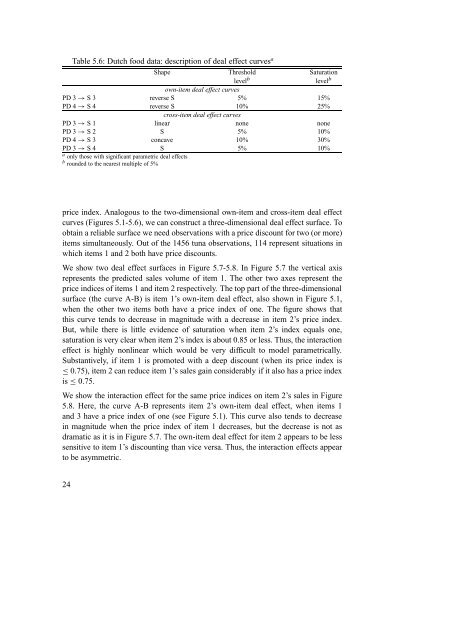
Table 5.6: Dutch food data: description of deal effect curves a Shape Threshold Saturation level b level b own-item deal effect curves PD 3 → S 3 reverse S 5% 15% PD 4 → S 4 reverse S 10% 25% cross-item deal effect curves PD 3 → S 1 linear none none PD 3 → S 2 S 5% 10% PD 4 → S 3 concave 10% 30% PD 3 → S 4 S 5% 10% a only those with significant parametric deal effects b rounded to the nearest multiple of 5% price index. Analogous to the two-dimensional own-item and cross-item deal effect curves (Figures 5.1-5.6), we can construct a three-dimensional deal effect surface. To obtain a reliable surface we need observations with a price discount for two (or more) items simultaneously. Out of the 1456 tuna observations, 114 represent situations in which items 1 and 2 both have price discounts. We show two deal effect surfaces in Figure 5.7-5.8. In Figure 5.7 the vertical axis represents the predicted sales volume of item 1. The other two axes represent the price indices of items 1 and item 2 respectively. The top part of the three-dimensional surface (the curve A-B) is item 1’s own-item deal effect, also shown in Figure 5.1, when the other two items both have a price index of one. The figure shows that this curve tends to decrease in magnitude with a decrease in item 2’s price index. But, while there is little evidence of saturation when item 2’s index equals one, saturation is very clear when item 2’s index is about 0.85 or less. Thus, the interaction effect is highly nonlinear which would be very difficult to model parametrically. Substantively, if item 1 is promoted with a deep discount (when its price index is ≤ 0.75), item 2 can reduce item 1’s sales gain considerably if it also has a price index is ≤ 0.75. We show the interaction effect for the same price indices on item 2’s sales in Figure 5.8. Here, the curve A-B represents item 2’s own-item deal effect, when items 1 and 3 have a price index of one (see Figure 5.1). This curve also tends to decrease in magnitude when the price index of item 1 decreases, but the decrease is not as dramatic as it is in Figure 5.7. The own-item deal effect for item 2 appears to be less sensitive to item 1’s discounting than vice versa. Thus, the interaction effects appear to be asymmetric. 24
Page 1 and 2: Semiparametric Analysis to Estimate
Page 3 and 4: 1. Introduction One of the key issu
Page 5 and 6: 2.3 Promotion signal effects Inman,
Page 7 and 8: it is important for researchers to
Page 9 and 10: nonparametric estimators, such as t
Page 11 and 12: applications in North America, Euro
Page 13 and 14: Table 4.2: Description of American
Page 15 and 16: (Table 5.2), while the Dutch food p
Page 17 and 18: 5.2 Predictive validity Since impro
Page 19 and 20: Figure 5.1: Tuna data: own-item dea
Page 21 and 22: Figure 5.3: Dutch food data: own-it
Page 23: 5.3.3 Key features We summarize key
Page 27 and 28: Figure 5.8: 3D tuna deal effect sur
Page 29 and 30: index is below 0.55. Thus the displ
Page 31 and 32: Appendix 1: Kernel method 10 Consid
Page 33 and 34: Appendix 2: Estimation procedure fo
Page 35 and 36: Appendix 3: Model operationalizatio
Page 37 and 38: are available for ˆm(x0). The esti
Page 39 and 40: Gupta, Sachin, Pradeep K. Chintagun

Semiparametric Analysis to Estimate the Deal Effect Curve

Create successful ePaper yourself

Delete template?

Save as template?