Chilling Tendency and Chill of Cast Iron

More documents

Recommendations

Info

180 2 Experimental Procedure 2.1 Flake graphite cast iron Experimental melts were made in a 15-kg capacity crucible of an electric induction furnace. The raw materials were pig iron, steel scrap, commercially pure silicon, and Fe-P and Fe-S alloys. Melting was followed by liquid iron superheating up to 1420℃ and inoculation using FOUNDRYSIL with a 0.2-0.5-cm granulation and added as 0.5 % of the total charge weight. After various time intervals (1.5, 5, 10, 15, 20, and 25 min) from the instant of inoculation, the cast iron was poured into plate shaped molds of s=0.6, 1.0, 1.6, 2.2, and 3.0 cm in thickness. The average chemical composition of cast iron was 3.18% C, 1.91% Si, 0.13% Mn, 0.092% P, and 0.064% S. In all cases, the plates had a common gating system. The foundry molds were prepared using conventional molding sand. In addition, they were instrumented with Pt/PtRh10 thermocouples enclosed in quartz sleeves. The thermocouple tips were located in the geometric center of each mold cavity. An Agilent 34970A electronic module was used to record the cooling curves which were used to determine the initial metal temperature Ti just after the mold filling and the maximum undercooling, 2.2 Ductile cast iron Tsinghua Science and Technology, April 2008, 13(2): 177-183 ∆Tm, at the onset of eutectic solidification. After cooling, specimens were taken for metallographic examination from the geometric centers of the plates. Metallographic examinations were made on polished and etched (stead reagent) specimens to show the graphite eutectic cell boundaries. The planar microstructure was characterized by the average number of eutectic cells NF per unit area (cell count) [12] N N + 0.5 N F + 1 i w F = (14) where Ni is the number of eutectic cells inside a rectangle S, Nw is the number of eutectic cells that intersect the sides of S but not their corners and F is the surface area of S. The average number of eutectic cells N per unit volume (volumetric cell count) was given by [13] N ≅ 0.568 N (15) 3/2 F Wedges with Bw=1.25 cm and α=28.5 o and samples for chemical composition measurement were also cast simultaneously with the plates. Figure 2 shows typical planar microstructures of the wedges. The width, W, of the total chill and the critical cell count, Ncr, were measured at the junction of the gray structure with the first spot of cementite as shown in Fig. 2. Fig. 2 Exhibited microstructure in wedge-shaped of flake graphite castings The test melts were made in an electric induction furnace having 8000 kg capacity. The raw materials were iron scrap, steel scrap, and commercially pure silicon. After melting and preheating at 1485 ℃ , the cast iron was poured into a casting ladle where it was spheroidized using the cored wired injection method. Different inoculants in various amounts were used. The aim of using different inoculants and inoculation processes was to induce different maximum undercoolings, ∆Tm, and various nodule counts N. The average chemical composition of the nodular iron was 3.69% C, 2.63% Si, 0.42% Mn, 0.02% P, 0.02% S, and 0.04% Mg. The nodular cast iron was poured into the same molds as for the gray cast iron. The cooling curves and metallographic structure were examined in the same way as for the gray cast iron. In the nodular cast iron the
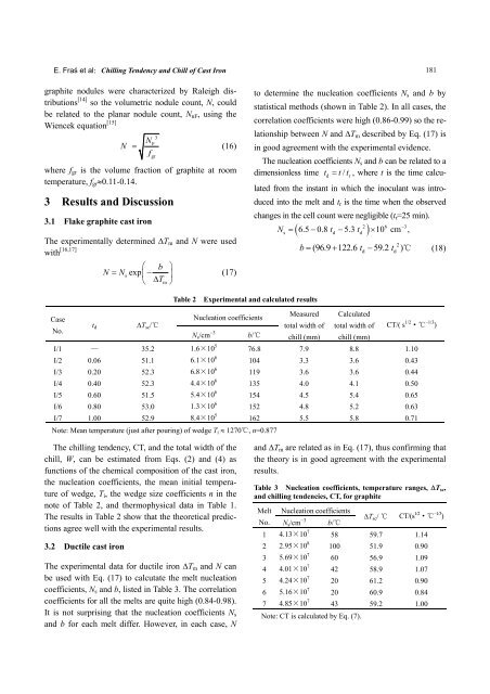
E. Fraś et al:Chilling Tendency and Chill of Cast Iron 181 graphite nodules were characterized by Raleigh distributions [14] so the volumetric nodule count, N, could be related to the planar nodule count, NnF, using the Wiencek equation [15] N 3 NF = (16) f where fgr is the volume fraction of graphite at room temperature, fgr≈0.11-0.14. 3 Results and Discussion 3.1 Flake graphite cast iron The experimentally determined ∆Tm and N were used with [16,17] Case No. td s gr ⎛ b ⎞ N = N exp − ⎜ ⎝ ∆Tm ⎠ ⎟ ∆Tsc/℃ (17) Table 2 Experimental and calculated results Nucleation coefficients Ns/cm −3 I/1 — 35.2 1.6×10 5 I/2 0.06 51.1 6.1×10 6 I/3 0.20 52.3 6.8×10 6 I/4 0.40 52.3 4.4×10 6 I/5 0.60 51.5 5.4×10 6 I/6 0.80 53.0 1.3×10 6 I/7 1.00 52.9 8.4×10 5 to determine the nucleation coefficients Ns and b by statistical methods (shown in Table 2). In all cases, the correlation coefficients were high (0.86-0.99) so the re- lationship between N and ∆Tm described by Eq. (17) is in good agreement with the experimental evidence. The nucleation coefficients Ns and b can be related to a dimensionless time t = t/ t , where t is the time calcu- d r lated from the instant in which the inoculant was intro- duced into the melt and tr is the time when the observed changes in the cell count were negligible (tr=25 min). b/℃ Note: Mean temperature (just after pouring) of wedge Ti ≈ 1270℃, n=0.877 The chilling tendency, CT, and the total width of the chill, W, can be estimated from Eqs. (2) and (4) as functions of the chemical composition of the cast iron, the nucleation coefficients, the mean initial temperature of wedge, Ti, the wedge size coefficients n in the note of Table 2, and thermophysical data in Table 1. The results in Table 2 show that the theoretical predictions agree well with the experimental results. 3.2 Ductile cast iron The experimental data for ductile iron ∆Tm and N can be used with Eq. (17) to calcutate the melt nucleation coefficients, Ns and b, listed in Table 3. The correlation coefficients for all the melts are quite high (0.84-0.98). It is not surprising that the nucleation coefficients Ns and b for each melt differ. However, in each case, N ( ) −3 N = 6.5 −0.8 t − 5.3 t × 10 cm , 2 6 s d d b= (96.9 + 122.6 t − 59.2 t ) ℃ (18) Measured total width of chill (mm) d Calculated total width of chill (mm) 2 d CT/( s 1/2 ·℃ –1/3 ) 76.8 7.9 8.8 1.10 104 3.3 3.6 0.43 119 3.6 3.6 0.44 135 4.0 4.1 0.50 154 4.5 5.4 0.65 152 4.8 5.2 0.63 162 5.5 5.8 0.71 and ∆Tm are related as in Eq. (17), thus confirming that the theory is in good agreement with the experimental results. Table 3 Nucleation coefficients, temperature ranges, ∆T sc, and chilling tendencies, CT, for graphite Melt Nucleation coefficients No. Ns/cm −3 1 4.13×10 7 2 2.95×10 8 3 5.69×10 7 4 4.01×10 7 5 4.24×10 7 6 5.16×10 7 7 4.85×10 7 b/℃ Note: CT is calculated by Eq. (7). ∆Tsc/ ℃ CT/(s 1/2 ·℃ –1/3 ) 58 59.7 1.14 100 51.9 0.90 60 56.9 1.09 42 58.9 1.07 20 61.2 0.90 20 60.9 0.84 43 59.2 1.00
Page 1 and 2: TSINGHUA SCIENCE AND TECHNOLOGY ISS
Page 3: E. Fraś et al:Chilling Tendency an
Page 7: E. Fraś et al:Chilling Tendency an

Chilling Tendency and Chill of Cast Iron

Create successful ePaper yourself

Delete template?

Save as template?