Introduction to Stochastic Loewner Evolution - University of Chicago
Introduction to Stochastic Loewner Evolution - University of Chicago
Introduction to Stochastic Loewner Evolution - University of Chicago

You also want an ePaper? Increase the reach of your titles
YUMPU automatically turns print PDFs into web optimized ePapers that Google loves.
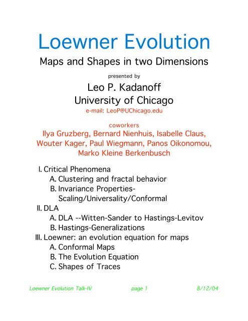
<strong>Loewner</strong> <strong>Evolution</strong><br />
Maps and Shapes in two Dimensions<br />
presented by<br />
Leo P. Kadan<strong>of</strong>f<br />
<strong>University</strong> <strong>of</strong> <strong>Chicago</strong><br />
e-mail: LeoP@U<strong>Chicago</strong>.edu<br />
coworkers<br />
Ilya Gruzberg, Bernard Nienhuis, Isabelle Claus,<br />
Wouter Kager, Paul Wiegmann, Panos Oikonomou,<br />
Marko Kleine Berkenbusch<br />
I. Critical Phenomena<br />
A. Clustering and fractal behavior<br />
B. Invariance Properties-<br />
Scaling/Universality/Conformal<br />
II. DLA<br />
A. DLA --Witten-Sander <strong>to</strong> Hastings-Levi<strong>to</strong>v<br />
B. Hastings-Generalizations<br />
III. <strong>Loewner</strong>: an evolution equation for maps<br />
A. Conformal Maps<br />
B. The <strong>Evolution</strong> Equation<br />
C. Shapes <strong>of</strong> Traces<br />
<strong>Loewner</strong> <strong>Evolution</strong> Talk-IV page 1 8/12/04
Abstract<br />
In statistical physics, a very considerable effort has<br />
gone in<strong>to</strong> studying the shapes <strong>of</strong> two-dimensional<br />
objects. especially fractals. Shapes <strong>of</strong> critical<br />
clusters are important in percolation and phase<br />
transitions, and in many dynamical problems.<br />
Conformal mappings in the complex plane provide<br />
another mechanism for producing shapes. This one is<br />
particularly natural for physics since analytic<br />
functions au<strong>to</strong>matically obey Laplace’s equation. This<br />
method has been directly used by Hastings and<br />
Levi<strong>to</strong>v <strong>to</strong> study DLA.<br />
<strong>Loewner</strong> devised a method <strong>to</strong> use conformal maps<br />
for constructing fractal line patterns. This method is<br />
described and explained. More recently <strong>Loewner</strong>’s<br />
method has been used <strong>to</strong> solve shape problems in<br />
percolation, self-avoiding walks, and critical<br />
phenomena. These applications are described.<br />
<strong>Loewner</strong> <strong>Evolution</strong> Talk-IV page 2 8/12/04
References<br />
T.A. Witten and L. Sander Diffusion-limited<br />
aggregation, a kinetic phenomenon. PRL 47, 1400,<br />
(1981).<br />
B. Duplantier Conformally Invariant Fractals and<br />
Potential Theory, PRL. 84, 1363 (2000); M. B.<br />
Hastings and L. S. Levi<strong>to</strong>v, Laplacian growth as onedimensional<br />
turbulence, Physica D 116, 244 (1998);<br />
arXiv:cond-mat/9607021.<br />
W. Werner, Critical exponents, conformal invariance<br />
and planar Brownian motion, arXiv:math.PR/0007042<br />
G. Lawler, <strong>Introduction</strong> <strong>to</strong> the SLE,<br />
http://www.math.duke.edu/~jose/papers.html.<br />
Leo P. Kadan<strong>of</strong>f & Marko Kleine Berkenbusch, Trace<br />
for the <strong>Loewner</strong> Equation with Singular Forcing,<br />
Nonlinearity, 17 4, R41-R54 (2004).<br />
Wouter Kager, Bernard Nienhuis, and Leo Kadan<strong>of</strong>f,<br />
Exact solutions for <strong>Loewner</strong> <strong>Evolution</strong>, Journal <strong>of</strong><br />
Statistical Physics, 115 3/4, 805-822 (May 2004)<br />
Ilya Gruzberg and Leo Kadan<strong>of</strong>f The <strong>Loewner</strong><br />
Equation: Maps and Shapes, Journal <strong>of</strong> Statistical<br />
Physics, 114 5, 1183-1198<br />
<strong>Loewner</strong> <strong>Evolution</strong> Talk-IV page 3 8/12/04
Preface<br />
Long ago, a bunch <strong>of</strong> us cracked the problem the<br />
theory <strong>of</strong> critical phenomena, or phase transition<br />
theory. We were able <strong>to</strong> describe how information<br />
about the system’s local order could be transferred<br />
<strong>to</strong> one part <strong>of</strong> the system <strong>to</strong> another, and especially<br />
how this information could be transferred over long<br />
distances near the critical point. The description was<br />
in terms <strong>of</strong> local quantities like density r(r) and<br />
magnetization s(r) at the point r and <strong>of</strong> correlations<br />
among these.<br />
A typical problem was the Ising model in which there<br />
was a lattice and at each lattice site there was a<br />
spin- variable, s(r), which <strong>to</strong>ok on the values plus<br />
one and minus one. Spins at neighboring sites were<br />
coupled <strong>to</strong>gether so that they tended <strong>to</strong> line up.<br />
The local alignment was strong at low temperatures<br />
and weak at high temperatures.<br />
The system has three phases: At high temperatures<br />
a disordered (paramagnetic phase) in which far<br />
distant points had no correlation. At low<br />
temperatures a ordered (ferromagnetic phase) in<br />
which correlation among spins extend over the entire<br />
system with a majority spins being (say) positive.<br />
<strong>Loewner</strong> <strong>Evolution</strong> Talk-IV page 4 8/12/04
At some intermediate temperature there is a critical<br />
phase in which large islands (domains) <strong>of</strong> spins tend<br />
<strong>to</strong> be lined up, but with the alignment getting weaker<br />
and weaker average as the clusters get larger.<br />
By 1975 or so we thought we were done. We<br />
unders<strong>to</strong>od how might depend upon the<br />
thermodynamic variables measuring distance from<br />
the critical point and how correlations like might behave.<br />
We also unders<strong>to</strong>od something about the basic<br />
global symmetries in the problem: the usual<br />
rotational and translational invariance, the spin-flip<br />
symmetry. At the critical point we saw in addition<br />
universality (rather different problems showed<br />
identical large-scale behavior), scaling (the large<br />
scale behavior was the same at all scales), and<br />
conformal invariance (a slight mysterious symmetry<br />
under complex analytic transformations <strong>of</strong> the<br />
space). So many <strong>of</strong> us went on <strong>to</strong> other things.<br />
But the old problem was not dead. We had left<br />
behind a crucial issue. How can one characterize the<br />
shapes <strong>of</strong> the spin clusters that form in critical<br />
phenomena? We did not even realize that we had<br />
left something behind.<br />
<strong>Loewner</strong> <strong>Evolution</strong> Talk-IV page 5 8/12/04
Percolation.<br />
Probability p that a site will be occupied (black)<br />
versus empty (red). Small p--small isolated clusters<br />
P close <strong>to</strong> one, same s<strong>to</strong>ry. If p is close <strong>to</strong> one half,<br />
lots <strong>of</strong> large clusters <strong>of</strong> both colors are formed<br />
<strong>Loewner</strong> <strong>Evolution</strong> Talk-IV page 6 8/12/04
In 1981 Witten & Sander developed a dynamical<br />
model called DLA. This model was intended <strong>to</strong><br />
construct scale-invariant, (fractal) objects. It did so,<br />
but despite a huge amount <strong>of</strong> work, we developed<br />
little understanding <strong>of</strong> the universality, scaling, or<br />
conformal properties <strong>of</strong> that model.<br />
Late in the 20th century, a new point <strong>of</strong> view was<br />
developed which enabled one <strong>to</strong> calculate the<br />
shapes <strong>of</strong> “domains”, i.e. correlated regions, in two<br />
dimensions. This point <strong>of</strong> view was somewhat<br />
mathematical in character and was in some sense<br />
invented by the mathematician Oded Schramm. I’ll<br />
try <strong>to</strong> tell about it and how it fits in <strong>to</strong> the other two<br />
development. trans,trans.<br />
On <strong>to</strong> DLA:<br />
DLA is a model invented by Witten and Sander <strong>to</strong><br />
describe how tiny bits <strong>of</strong> soot may come <strong>to</strong>gether<br />
and form one large, fractal aggregate. It was one <strong>of</strong><br />
the first models <strong>to</strong> be initially expressed as a<br />
computer algorithm trans,trans.<br />
<strong>Loewner</strong> <strong>Evolution</strong> Talk-IV page 7 8/12/04
Conformal Maps<br />
We don’t teach much complex analysis <strong>to</strong> physics<br />
students. So I’ll say some elementary things here.<br />
r<br />
A point r = (x,y) can also be written as z=x+iy. A<br />
bunch <strong>of</strong> points define a shape. Take z=e iq = cos q +<br />
i sin q with q between 0 and 2 π and you get a circle.<br />
†<br />
z<br />
Functions <strong>of</strong> a complex variable au<strong>to</strong>matically obey<br />
Laplace’s equation at every point where there is no<br />
singularity. If w=1/z=1/(x+iy) =(x-iy)/(x 2 +y 2 ) then<br />
we au<strong>to</strong>matically know that<br />
[(∂ x) 2 +(∂ y) 2] [x/(x 2 +y 2 )] =0<br />
except at z=0.<br />
<strong>Loewner</strong> <strong>Evolution</strong> Talk-IV page 8 8/12/04
D<br />
Here is another curve. It sits in the z-plane. Let<br />
w=f(z)=(z+1/z)/2. What do you get? Take the<br />
curvey part described by z=e iq with q real and in<br />
[0,π]. Plug this in<strong>to</strong> f. All these points <strong>to</strong>gether give<br />
a line segment, w=cos q. Now take the right hand<br />
straight part given by z=e u, u>0. This gives a line<br />
segment, w=cosh u, extending from 1 <strong>to</strong> infinity. All<br />
<strong>to</strong>gether you get the shape shown below.<br />
R w<br />
What we have just done? We have constructed a<br />
conformal mapping, which takes the colored curve in<br />
the z-plane in<strong>to</strong> the line in the w-plane. It also takes<br />
the region above the curve in z, D, in<strong>to</strong> the region<br />
above the line in w, R, in a one <strong>to</strong> one manner.<br />
<strong>Loewner</strong> <strong>Evolution</strong> Talk-IV page 9 8/12/04<br />
z
Definition: Conformal Map<br />
A conformal mapping, is a function f(z) analytic<br />
within a simply connected region D <strong>of</strong> the complex zplane,<br />
and which has the property that df/dz is never<br />
zero in D. It then provides a one-<strong>to</strong>-one mapping <strong>of</strong><br />
the interior <strong>of</strong> D in<strong>to</strong> the interior <strong>of</strong> another simply<br />
connected region R and likewise maps the curves<br />
which bounds these regions in<strong>to</strong> one another.<br />
Riemann proved that for finite regions the mapping is<br />
unique. To go backwards from R <strong>to</strong> D you use the<br />
inverse function g(w) which obeys g(f(z))=z. This<br />
<strong>to</strong>o is unique.<br />
In the complex plane analysis and geometry are the<br />
same thing.<br />
<strong>Loewner</strong> <strong>Evolution</strong> Talk-IV page 10 8/12/04
Going Backwards<br />
w=f(z)=(z+z -1)/2 takes D in<strong>to</strong> R.<br />
D<br />
R<br />
Solve for z.<br />
in<strong>to</strong> D.<br />
Note that non-analyticity at w=1,-1, z=0 and<br />
†<br />
vanishing derivatives z=1,-1 at all give interesting<br />
behavior.<br />
w<br />
z = w + w 2<br />
-1 z=g(w) Then g takes R<br />
<strong>Loewner</strong> <strong>Evolution</strong> Talk-IV page 11 8/12/04<br />
z
Composition Properties<br />
w=f1(z)=(z+z -1)/2 takes D 1 <strong>to</strong> R.<br />
w=f2(z)=[(z-0.5+(z-0.5) -1]/2 takes D 2 <strong>to</strong> R.<br />
D 2<br />
D 1<br />
w=f2(f1(z))=takes a larger region <strong>to</strong> R.<br />
<strong>Loewner</strong> <strong>Evolution</strong> Talk-IV page 12 8/12/04<br />
z<br />
z
†<br />
†<br />
Diffusion Limited Aggregation, Again<br />
One can equally well form DLA aggregates by doing<br />
a bump map many many times. On picks a map <strong>of</strong><br />
the form<br />
w = fa(z) = (z- a + r2<br />
)/ 2,<br />
z - a<br />
which makes bumps with radius r and position a. (r<br />
and a must be real.) The one puts <strong>to</strong>gether a bunch<br />
<strong>of</strong> bumps by successively forming the maps one<br />
after the other:<br />
F(z) = fa5 ( fa4 ( fa3 ( fa2 ( fa1 (z)))))<br />
One bump:<br />
many bumps tend <strong>to</strong> clump<br />
trans<br />
<strong>Loewner</strong> <strong>Evolution</strong> Talk-IV page 13 8/12/04
Basic math behind this: (Hastings and Levi<strong>to</strong>v) The<br />
probability for finding a random walker someplace is<br />
defined by a diffusion process, which thus obeys the<br />
discrete analog <strong>of</strong><br />
[(∂ x) 2 +(∂ y) 2] p(x,y)=0<br />
with the relative probability, p(x,y), being zero on<br />
the aggregate. The actual probability <strong>of</strong> hitting is<br />
the value <strong>of</strong> the probability on a site next <strong>to</strong> the<br />
aggregate, which is proportional <strong>to</strong> the normal<br />
gradient <strong>of</strong> the probability at the aggregate.<br />
Using complex analysis we know precisely how <strong>to</strong><br />
construct such a function. Take our strange shaped<br />
object. Let the outside <strong>of</strong> that object be the region<br />
R in the z plane. Construct the map which takes R<br />
in<strong>to</strong> the upper half <strong>of</strong> the w-plane. The map gives p:<br />
w=f(z)=f(x+iy)=q(x,y)+ip(x,y).<br />
To check note that f(z) obeys the Laplace equation,<br />
is real on the boundary and has the right behavior at<br />
infinity.<br />
<strong>Loewner</strong> <strong>Evolution</strong> Talk-IV page 14 8/12/04
Physical models:<br />
DLA: bumps appear at random positions in w, all<br />
equal in size. (Hastings and Levi<strong>to</strong>v)<br />
Noise-reduced DLA: many hits in the neighborhood<br />
<strong>of</strong> a given w are required before a bump is raised.<br />
Chao Tang: result is different.<br />
Other models: bump size =1. New bump is produced<br />
at a “distance” Dw = k 0.5 from last bump and a<br />
random direction. This random walk produces fractals<br />
very different from DLA. Structure <strong>of</strong> fractals differs<br />
depending on value <strong>of</strong> k (Oded Schramm had the<br />
basic insights, further developed by Lawler and<br />
Warner, and then Hastings translated them in<strong>to</strong> this<br />
language.)<br />
<strong>Loewner</strong> <strong>Evolution</strong> Talk-IV page 15 8/12/04
†<br />
On <strong>to</strong> <strong>Loewner</strong><br />
There is a connection between the work <strong>of</strong> Hastings<br />
and Levi<strong>to</strong>v and the much earlier work <strong>of</strong> C. <strong>Loewner</strong><br />
who was studying the generation <strong>of</strong> singularities in<br />
conformal maps. He looked at the map f t(z) and<br />
asked himself how he could produce smooth<br />
deformations <strong>of</strong> this map. As part <strong>of</strong> this he turned<br />
<strong>to</strong> consideration <strong>of</strong> the equation<br />
d<br />
dt<br />
f t(z)<br />
=<br />
2<br />
f t - x(t)<br />
with the initial condition f 0(z)=z<br />
Here f and z are complex, t and x are real. The time<br />
development <strong>of</strong> f(z), as generated by this equation<br />
is called the <strong>Loewner</strong> evolution.<br />
This equation has been used <strong>to</strong> prove some<br />
important and fundamental propitious <strong>of</strong> analytic<br />
functions. However, we wish <strong>to</strong> look at it from a<br />
geometrical point <strong>of</strong> view: w=f t(z) is a mapping<br />
which takes you from a point z in region, D,<br />
contained in the upper half <strong>of</strong> the z-plane <strong>to</strong> another<br />
region R which is the upper half <strong>of</strong> the w plane. The<br />
geometry <strong>of</strong> D is the primary focus <strong>of</strong> our interest.<br />
At time zero the geometry is simple, f=z and D=R.<br />
<strong>Loewner</strong> <strong>Evolution</strong> Talk-IV page 16 8/12/04
†<br />
The simplest case<br />
The simplest case, x(t)=x(0)=x 0, is quite instructive.<br />
The equation is: df/dz=2/(f -x 0) or d ((f -x 0) 2)/dt=4<br />
so that [f t(z)-x 0] 2 =4t+c(z) where c is a “constant”<br />
<strong>of</strong> integration. The initial condition, f=z then, implies<br />
ft (z)- x0 = (z -x 0 ) 2 + 4t . This solution has a branch cut,<br />
at which the square root changes sign, running up a<br />
line Re z=x0 from z=x0 <strong>to</strong> z=x0+2i t . The region D is<br />
the upper half plane less the branch cut.<br />
†<br />
A<br />
One can work with these line segments in just the<br />
same way as Hastings worked with bumps. One<br />
again the function <strong>of</strong> a function composition works <strong>to</strong><br />
give more complex structures from simpler ones.<br />
B<br />
C<br />
A B C<br />
<strong>Loewner</strong> <strong>Evolution</strong> Talk-IV page 17 8/12/04<br />
z<br />
w
More On <strong>Loewner</strong><br />
What a bore! All this work and you get a line<br />
segment. And it gets worse. If x(t) is any smooth<br />
x(t)- x(s)<br />
curve with lim 1/2 = 0 then the geometrical<br />
tÆs (t - s)<br />
object generated is just a curvey line. For example,<br />
for x(t) =t, the trace looks like trans<br />
However, † all this dullness is, if seen the right way,<br />
quite exciting. The <strong>Loewner</strong> equation can be seen<br />
as a machine for producing a curve called a trace<br />
which depends upon the forcing function x(t). This<br />
machine has quite fantastic qualitative properties,<br />
which depend almost entirely upon the singularity<br />
structure <strong>of</strong> x(t). This is exciting in itself.<br />
The form <strong>of</strong> the trace has simple covariance<br />
properties under the operation <strong>of</strong> translation,<br />
rotation, and scale change.<br />
<strong>Loewner</strong> <strong>Evolution</strong> Talk-IV page 18 8/12/04
xy plot <strong>of</strong> trace<br />
Wouter Kager 7/03<br />
x(t) = t<br />
<strong>Loewner</strong> <strong>Evolution</strong> Talk-IV page 19 8/12/04
For smooth forcing functions<br />
The trace is non-self-interecting and does not<br />
intersect the real axis.<br />
Essentially any such curve can be generated in this<br />
fashion<br />
If the forcing is sufficiently singular, one can<br />
generate other shapes. If we have x(t) = 2[k(1- t)] b<br />
then if b < 1/2 the trace will intersect itself.<br />
•For b = 1/2 and k < 4 we get a logarithmic spiral<br />
which circles around and infinite † number <strong>of</strong> times.<br />
trans<br />
•For b = 1/2 and k > 4 we get an intersection with<br />
the real line trans,trans,trans,<br />
• For b = 0, i.e. discontinuous forcing, one can get<br />
discontinuous traces. trans,<br />
We have had lots <strong>of</strong> fun with this*, but let me move<br />
on <strong>to</strong> other things<br />
*coworkers: Bernard Nienhuis, Isabelle Claus, Wouter<br />
Kager, Panos Oikonomou, Marko Kleine Berkenbusch<br />
<strong>Loewner</strong> <strong>Evolution</strong> Talk-IV page 20 8/12/04
<strong>Loewner</strong> <strong>Evolution</strong> Talk-IV page 21 8/12/04
<strong>Loewner</strong> <strong>Evolution</strong> Talk-IV page 22 8/12/04
On <strong>to</strong> S<strong>to</strong>chastic <strong>Evolution</strong>...<br />
The real fun comes when the forcing function is<br />
s<strong>to</strong>chastic. The first hint <strong>of</strong> this came from Hastings<br />
and Levi<strong>to</strong>v and DLA.<br />
To S<strong>to</strong>chastic <strong>Loewner</strong> <strong>Evolution</strong>... SLE<br />
Look at the traces induced by the s<strong>to</strong>chastic version<br />
<strong>of</strong> the <strong>Loewner</strong> equation in which the forcing is the<br />
Gaussian random process x(t)= k B(t) where B<br />
represents normalized Brownian motion. Specifically<br />
= k |t-s|<br />
There are several qualitatively different forms <strong>of</strong> the<br />
traces depending upon the values <strong>of</strong> k.<br />
The results are spectacular.<br />
We have already seen that if we chose x(t) <strong>to</strong> be a<br />
smooth real-valued function, the mapping f t(z) would<br />
give a conformal map from the upper half-plane, with<br />
a simple curve cut away. However because a<br />
Brownian walk contains small-scale singularities, we<br />
cannot be sure a priori what will happen. Indeed the<br />
RMS separation [x(t)-x(s)] is (k |t-s|) 1/2 which is just<br />
marginal for singularity production. What happens has<br />
been sorted out by some elegant mathematics,<br />
which shows that the result depends on k.<br />
<strong>Loewner</strong> <strong>Evolution</strong> Talk-IV page 23 8/12/04
What Happens<br />
is that the SLE process cuts away some portion <strong>of</strong><br />
the z-plane. For 0< k ≤ 4 the SLE trace is a non-selfintersecting<br />
curve<br />
for 4< k ≤ 8 a self-intersecting one and for 8
<strong>Loewner</strong> <strong>Evolution</strong> Talk-IV page 25 8/12/04
<strong>Loewner</strong> <strong>Evolution</strong> Talk-IV page 26 8/12/04
More problems solved<br />
• Similarly, the percolation problem has a solution<br />
related <strong>to</strong> k = 6 SLE. In the scaling limit, critical<br />
percolating clusters have the same ensemble <strong>of</strong><br />
shapes as the exterior boundaries <strong>of</strong> the intersecting<br />
SLE paths.<br />
These results are theorems. Next comes a bunch <strong>of</strong><br />
very plausible speculations about the relation<br />
between SLE and the critical limit <strong>of</strong> phase transition<br />
problems. Concretely the speculation is that the<br />
ensemble <strong>of</strong> all SLE shapes give the shapes <strong>of</strong> the<br />
outline <strong>of</strong> clusters <strong>of</strong> the critical points <strong>of</strong> different<br />
phase transition problems. Specifically, k=3<br />
corresponds <strong>to</strong> the Ising model.<br />
Finally <strong>Loewner</strong> evolution au<strong>to</strong>matically give<br />
information about the electric field singularities which<br />
emerge when LE and SLE geometrical objects are<br />
taken <strong>to</strong> be charged conduc<strong>to</strong>rs. Judging from DLA,<br />
these questions about charging are quite relevant <strong>to</strong><br />
the deeper geometrical meaning <strong>of</strong> these objects.<br />
The work <strong>of</strong> Duplantier on the electrical properties <strong>of</strong><br />
critical clusters actually came before SLE but it has a<br />
similar spirit.<br />
<strong>Loewner</strong> <strong>Evolution</strong> Talk-IV page 27 8/12/04