Turbulent Heat Flow: Structures and Scaling - University of Chicago

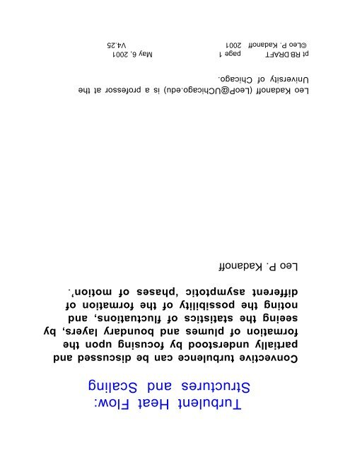
pt RB DRAFT page 1 May 6, 2001 

©Leo P. Kadanoff 2001 V4.25 

Leo Kadanoff (LeoP@UChicago.edu) is a professor at the 

University of Chicago. 

Convective turbulence can be discussed and 

partially understood by focusing upon the 

formation of plumes and boundary layers, by 

seeing the statistics of fluctuations, and 

noting the possibility of the formation of 

different asymptotic ‘phases of motion’. 

Turbulent Heat Flow: 

Structures and Scaling 

Leo P. Kadanoff

pt RB page 2 May 6, 2001 

2 Lord Rayleigh, On Convection Currents in a Horizontal Layer of Fluid, when the higher 

temperature is on the under side, Philos. Mag. 32 529 (1916). H. Bénard, Les tourbillons 

cellulaire dans une nappe liquide, Rev. Gen. Sci. Pur. Appl. 11 1261 (1900). 

1 A good recent review is Eric D. Siggia, High Ra Number Convection, Annual Reviews of 

Fluid Mechanics 22 137-168 (1994). Many recent references can be found in Siegfried 

Grossmann and Detlef Lohse, Scaling in thermal convection: a unifying theory, J. Fluid Mech. 

407 27-56 (2000). For a popular treatment see L.P. Kadanoff, A. Libchaber, E. Moses and G. 

Zocchi, Turbulence dans une Boîte, La Recherche, 22 628-638 (1991). 

Geometrical Structures: Plumes, Flywheels, and More 

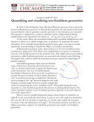
We want to understand the flow pattern depicted in Figure 1. From studies 

of other fluid flows, we expect our flow to contain reasonably welldefined 

structures, appearing in a mosaic of different combinations and 

Turbulence can be seen in the wind and the water all around us. Swirls of 

winds are proverbially inconstant. The pattern changes and changes and 

changes again. Nonetheless, wind is in some sense always the same. Its 

average and statistical properties are predictable. There are at least four 

strategies which will isolate features of turbulent flows for scientific 

study. One is to look for the qualitative geometry of characteristic 

structures which recurringly appear in the flow. The second is to analyze 

fluctuations, looking for characteristic probability distributions. A third 

is to obtain quantitative characterizations of the average flows. Finally, 

one can study time series and their Fourier transforms. In each case, we 

are trying to isolate elements of the flow which are open to prediction, 

replication, and comparison among different systems. We shall look at the 

first three here, but put aside the last one for lack of space. 

For very many years scientists have studied the motion of enclosed fluids 

heated from below and cooled from above1. The containers for these 

Rayleigh Bénard systems2 have ranged in size from coke cans to swimming 

pools. Usually, as a fluid is heated it will become less dense. A heated blob 

will feel a force pushing it upwards, the blob will tend to rise and cooler 

fluid will fall into its place. At the lowest heating rates there is no 

motion. Then as the heating rate is increased one sees successively a 

steady motion, a periodic oscillation, and a chaotic domain. At higher 

heating rates, one finds a turbulent motion in which the fluid swirls in 

highly structured but never-repeating patterns. (See Figure 1.)


So the heat flow has created a ‘machine’ containing many different 

working parts: boundary layers, mixing zones, jets, a central region. Figure 

4 is a cartoon of the machinery at work. Start at the lower left hand 

corner of the cell. A wind produces flow progressing from left to right, 

and carrying with it some waves. Here, the waves are bulges in the height 

of the thin boundary layer at the bottom of the cell. As they move, the 

waves throw up a hot spray which tends to rise, forming sheets of hot 

Figure 1 shows a small container heated carefully and uniformly from 

below, cooled from above and illuminated with a nearly parallel light 

beam. Inhomogeneities in temperature bend the light and produce the 

shadows shown. As you can see, the container is filled with plumes. Hot 

plumes congregate in an upwelling jet of fluid near the right-hand wall of 

the container. A similar, downward jet formed from cold plumes occurs 

on the left-hand wall. Large numbers of hot plumes are also found in left 

to right motion in a ‘mixing zone’ or viscous boundary layer near the 

bottom of the container. A similar layer on the top contains cold plumes, 

moving in the opposite direction. The central region contains a few 

plumes, hot and cold, in a partially random motion. These plumes wander 

chaotically but also participate in an overall counterclockwise motion. In 

addition, there are very thin boundary layers, not really visible in the 

present picture, near the top and bottom walls. The majority of the 

temperature drop between bottom and top of the container occur within 

these thermal boundary layers. 

One structure often found in heated fluids is called a plume. As heated 

fluid rises, it pushes aside fluid above it and is in turn deflected by this 

pushing. The rising fluid produces a little stalk, like the base of a 

mushroom, while the deflected fluid produces a cap on top. As the pushing 

and deflection continue, the edge of the cap may further fold over. The 

result is something that looks like a mushroom. The nuclear explosion of 

Figure 2 shows a very large plume produced by rising gases. Yet larger 

plumes are depicted in Figure 3, which is reproduced from a computer 

simulation of the surface of the sun. This picture shows many cold plumes 

falling downward into the sun. More mundane plumes can be seen in a wide 

variety of laboratory pictures and simulations. 

ever changing patterns.


The critical reader will recognize that the analysis up to this point has 

been rather subjective. I could have told another story, focusing upon 

different features of the flow, and perhaps come to different lessons. 

Nonetheless, a multiplication of examples might help the reader believe 

that these words catch some properties of ‘complex systems’. 

Lesson III: Big events happen. The flywheel motion can persist in the 

same direction through very many rotations . But once in a while the 

motion will reverse itself, in a large and quite exceptional event. 

Lesson II: Interesting and persistent structures can exist and persist in a 

noisy environment. Here, the structures include both the plumes and the 

counterclockwise flywheel motion of the entire fluid. 

Lesson I: A nonequilibrium system can organize itself in an amazing 

fashion, producing a sort of machine with many different working parts 

each serving an apparent function. This natural tendency toward selforganization 

might perhaps have some role in creating the intricate 

machinery of biological systems. 

The story: A cell is filled with a fluid. The fluid is strongly heated from 

below. Buoyancy raises the heated material and a flow starts. 

So we have a story and a few lessons. 

upward motion. These sheets break up into columnar structures which 

form the plumes shown in Figures 1 and 4. As they move across the bottom 

of the cell, these structures grow larger. (See Figure 5.) A few plumes 

come loose and move into the central region. Most hit the right-hand wall 

and move upward as a jet aimed toward the top of the cell. As a plume hits 

the upper wall, it makes a splash. The splash makes a wave. Each wave 

moves along the top, producing cold spray and thence cold plumes. The 

plumes form into a downward jet at the left hand side, splash on the 

bottom, and produce hot waves....... The jets thus pull the fluid around the 

container, forming a liquid flywheel. We find an intricate motion, which 

has the seeming purpose of moving heat from the bottom of the container 

to the top.


3 J Boussinesq Theorie Analytique de la Chaleur (Gauthiers-Villars, Paris, 1903) Vol. 

The basic equations: 

We do have specific and exact knowledge of hydrodynamics. We know the 

partial differential equations obeyed by any fluid in which variations in 

space and time are sufficiently slow. These equations describe the flow of 

energy, momentum, and particles through the system. They relate rates of 

change in time to rates of change in space for velocity, u, temperature, T, 

and pressure, p. If the density change is sufficiently gentle, the full fluid 

equations can be simplified to the Boussinesq3 equations: 

2.


4 For example, (a) Robert M. Kerr and Jackson R. Herring, Prandtl number dependence 

of Nusselt number in direct numerical simulations, Journal of Fluid Mechanics (2000), 

419:325-344. (b) R. Verzicco and R. Camussi, Prandtl number effects in convective 

turbulence, J. Fluid Mech. 383 55-73 (1999). (c) R. Camussi and R. Verzicco, Convective 

turbulence in Mercury: Scaling laws and spectra, Physics of Fluids 10 516-527 (1998). It 

is interesting to note how authors of simulational papers have adopted the language of 

experimental science. “Several probes are placed inside...” op. cit.. p 517. 

where L is the size of the container and ΔT is the temperature difference 

across it. All containers of fixed shape and obeying the same boundary 

conditions will have their flow properties completely determined by these 

two numbers. 

Another very solid prediction can be made by converting these equations 

for the Rayleigh Bénard cell into dimensionless form. For a given shaped 

box the equations will then depends upon two dimensionless parameters: 

the Prandtl number, Pr, which measures the relative propensity of the 

fluid to diffuse momentum versus heat, and the Rayleigh number, Ra, 

characterizing the strength of the heat flow driving the turbulence. In 

symbols 

3 

(2) Ra = 

g α L 

ΔT Pr = υ / κ 

Indeed, Figure 3 was generated in a computer simulation using a variant 

of these equations. From many similar observations and simulations, we 

certainly know that plumes are a consequence of the Boussinesq equations. 

coefficient, thermal diffusivity, and kinematic viscosity of the fluid, 

while g is the acceleration of gravity. Equations (1) have a very different 

status from the ‘lessons’ given above. The equations have been checked 

experimentally, studied theoretically, and used for many years in 

simulations4. They are an essential part of our accumulated knowledge of 

fluids. 

Here ρ, α, κ, and υ are respectively the density, thermal expansion 

∇ . u = 0 

T + (u ∇ )T = κ ∇ 

t 2 T 

u t + (u . ∇ ) u = − ( ∇ p) / ρ + υ ∇ 2 u + α g T 

κυ 

(1)


6 Y.-B. Du and P. Tong, Temperature Fluctuations in a Convective Cell with Rough Upper 

and Lower Surfaces, Phys Rev E 63 046303 (2001). For earlier work see, for example, 

references 8 and 11. 

Phys. Rev. E 49, 2912–2927 (1994). 

5 B. Shraiman, E. Siggia, Lagrangian path integrals and fluctuations in random flow, 

exponential of -|Δ| p . Experiments6 show that just below the onset of 

turbulence, p is two, while p is close to 1.0 in the lower part of the 

strongly turbulent range (see Figure 7), and about 1.5 in a higher range of 

Ra. Smaller p means that big fluctuations are more likely. The increased 

likelihood of extreme events can have extreme consequences. For 

example, if you were an engineer designing an airplane part with a 

potential for causing in-flight failure, you might consider it to be 

conservative if you designed for safety against all but a ten-standard 

deviation event. Indeed with a Gaussian pattern that event would have a 

exponential of a constant times -Δ2 . However, in this and other turbulent 

flows there is an increased likelihood for large fluctuations, which is 

indicated by a probability distribution that falls off much more slowly 

than a Gaussian. Specifically, the distribution is proportional to an 

liberated from far away5 . One can make this point more quantitative by 

examining plots of the probability distribution for observing a given 

temperature as a function of the deviation of that temperature from its 

average value. Since the time of Galton and Gauss, people have assumed 

that under most circumstances the probability distribution for a deviation 

of size Δ will have a Gaussian form, i.e. that it will be proportional to an 

Our convective cell shows another kind of anomalously large fluctuation. 

The temperature in the central region shows an occasional very large 

excursion, probably as the result of the occasional passage of fluid newly 

Statistical patterns 

Lesson III above says that we should expect extreme events. In fact, large 

excursions are a regular feature of the behavior of turbulent systems. Our 

system has a flywheel motion which undergoes an occasional turnaround, 

roughly similar to the occasional turnaround in the earth’s magnetic field. 

Many complex things undergo sudden large changes, producing outcomes 

like tornados, or earthquakes, or rapid global warming.


8 B. Castaing, G. Gunaratne, F. Heslot, L.P. Kadanoff, A. Libchaber, S. Thomae, X.-Z. Wu, 

S. Zaleski and G. Zanetti, J. Fluid Mechanics 209 1-30 (1989). 

7 Corey S. O’Hern, Stephen A. Langer, Andrea J. Liu and Sidney R. Nagel, Force 

Distributions Near Jamming and Glass Transition, Phys. Rev. Lett. 86 111-114 (2001), 

which also contains references to earlier works. 

In one such approach, a University of Chicago collaboration8 identified 

the different layer regions shown in Figure 4 and then estimated typical 

velocities, temperature differences, and region-sizes to obtain a power 

law with β=2/7, fitting the then-existing data and some more recent data 

(3a) Nu = A Ra β + ... 

There are many theories which begin from a picture of the different 

regions within the convective cell and then estimate the order of 

magnitude of the various velocities and temperature in each region. In 

theories of this type it is traditional to guess that there is simple scaling 

so that one can fit the behavior by power laws of the form 

Algebraic Features. 

The total amount of heat flowing upward through the convective cell is 

measured by the Nusselt number, Nu, which is the ratio of the actual heat 

flow to the flow which would occur via heat conduction alone. The motion 

of the fluid enables Nu to become increasingly large as the Rayleigh 

number increases. (See Figure 6). 

An exponential tail appears to be a characteristic feature of many 

physical situations. Exponentials are seen, for example, in force 

distributions in glassy materials, foams, and sand piles7. We do not 

understand why they appear so often. 

probability of one chance in 1022 or thereabout of occurring. That is 

almost certainly good enough. With an exponential distribution, 

unfortunately, the catastrophic event has a likelihood 1/20,000. A big 

difference.


11 J.J. Niemela, L. Skrbek, K.R. Sreenivasan, R.J. Donnelly “ Turbulent convection at 

very high Rayleigh numbers” Nature 404 837-840 and private communication. These 

authors ascribe equation (3c) to Howard, Roberts, Stewartson and Herring and to J. Toomre, 

D.O. Gough and E.A. Spiegel, Numerical solution of single-mode cavity equation, J. Fluid Mech. 

79 1-31 (1977). 

Convection, Phys. Rev. Lett. 84, 4357 (2000). 

10 X. Xu, K.M.S. Bajaj, and G. Ahlers, Heat Transport in Turbulent Rayleigh-Bénard 

9 See also B. Shraiman and E. Siggia, Heat transport in high-Rayleigh-number 

convection, Phys. Rev. A 42, 3650 (1990). On the experimental side see for example Shay 

Ashkenazi and Victor Steinberg, High Rayleigh Number Turbulent Convection in a Gas near the 

Gas-Liquid Critical Point, Phys. Rev Lett. 83, 3641-3644 (1999). 

A different perspective might be in order. None of these equations mean 

anything in themselves. To give them meaning, you have to define the 

Before choosing it is reasonable to ask “what are we trying to do?”. If our 

goal is to get a decent representation of the facts observed in a very wide 

range of turbulence experiments, all three formulas are acceptably good. 

from a theory based upon the flow though one ‘optimum’ mode. They also 

point to an equally good fit via equation (3a) with β=0.309. All these 

proposed formulas match the data to a respectable accuracy. (See 

Figure 6.) How to choose? 

+ ... , 

(3c) Nu = A Ra 3 / 2 (ln Ra) 

Equation (3a) assumed a more or less serial process of heat-movement 

from boundary layer to mixing zone to central region, while (3b) assumes a 

pair of processes working in parallel to produce his two terms. Other fits 

are possible. Niemela et al11 note a good fit, 

(3b) Nu = A Ra 1 / 3 + B Ra 1 / 4 + ..... 

For example in a recent paper, X. Xu, K.M.S. Bajaj, and G. Ahlers10 get an 

excellent fit using the Grossmann-Lohse suggestion1 pretty well 9 . Other ‘laws’ seem to do the same job, perhaps even better. 

1 / 5


Shraiman and Siggia reference 9. 

15 Emily Ching, private communication. See also Grossmann and Lohse reference 1 and 

Fluids 5, 1374-1389 (1962). 

14 R.H. Kraichnan, Turbulent thermal convection at arbitrary Prandtl number Phys. 

13 Scientists often frame their arguments with a view to how the theory might, in the 

end, work out. (See for example Stephen Weinberg Dreams of a Final Theory (Vintage,1994) ) 

We imagine that there is an unambiguous answer, that it is relatively simple, knowable, and 

will finally be known. A similar view is presented by almost all detective stories, as for 

example, Josephine Tey, The Daughter of Time (Berkeley,New York, 1951). However, outside 

the sciences, answers are usually more ambiguous--indeed often unknowable. (See, for 

example, Michael Frayn, Copenhagen, (Anchor,2000).) 

12 For a novel suggestion in that direction see a recent preprint by Bérengère Dubrulle. 

behavior with β=1/2. (plus logarithmic corrections). However, Kraichnan, 

and more recent authors15 have argued that this “ultimate” regime 

asymptotic regimes14 . One regime is very, very high Rayleigh number, with 

a non-extreme value of the Prandtl number. In that case, Kraichnan said 

that highly energetic turbulent events would destroy much of the 

structure shown in figure 1, and give processes in which globs of hot fluid 

would move from bottom to top in an almost ballistic fashion, trading 

their gαΔΤ potential energy for kinetic energy, thereby generating a 

One possible description of such an eventual theory might be discerned in 

Robert Kraichnan’s work of 1962, which outlines three different 

terms ‘+...’, appearing in both equations. In my view, the right thing is to 

demand that the fit become asymptotically accurate. I mean that there 

should be some limiting process in which the proposed theory would be 

exactly true12. The limiting process would most likely involve having the 

Rayleigh number go to infinity, with maybe also having the Prandtl number 

going to some extreme value. Alternatively, some fluctuations or 

processes might be neglected. Then the ‘+...’ would represent the 

corrections to this asymptotic result and could be given a well-defined 

meaning. So I am suggesting that, to fit the data, one should look forward 

and guess the form of the eventual mathematical theory which will 

describe what really happens in the system in some very extreme limit13.


18 P.-E. Roche, B. Castaing, B. Chabaud, and B. Hébral, Observation of the power law in 

Rayleigh-Bénard convection Phys. Rev E63 045303 (2001). 

17 X. Chavanne, F. Chillà, B. Castaing, B. Hébral, B. Chabaud, and J. Chaussy, 

Observation of the Ultimate Regime in Rayleigh-Bénard Convection, Phys. Rev. Lett. 79, 

3648–3651 (1997). 

16 S. Cioni, S. Ciliberto, and J. Sommeria , Strongly turbulent Rayleigh–Bénard 

convection in mercury: comparison with results at moderate Prandtl number, Journal of Fluid 

Mechanics 335 111-140 (1997). See also in contrast T. Takeshita, T. Segawa, J. Glazier, M. 

Sano, Thermal turbulence in mercury, Phys. Rev. Lett. 76 1465-1468 (1996). 

The theories which characterize the different asymptotic regimes all 

include some scaling characterizations of the different regions and 

structures within the flow. Thus detailed measurements of temperatures 

and velocities as a function of position within the cell can serve to 

could tip the convective behavior into different asymptotic regimes 18 . 

the same range of Ra in which reference 11 finds β=0.309. Such 

differences would be understandable if a difference in boundary conditions 

Mercury. In Helium, Chavanne, et. al 17 observe a β=1/2 regime in exactly 

There is indirect experimental evidence which tends to support the notion 

of several asymptotic regimes. Different experimental groups can observe 

different apparent values of the index β. This can even happen when they 

are working with the same fluid and the same value of Ra, but have cells 

which differ in geometry or in boundary behavior. Footnote 16 refers to 

papers which show such a ‘discrepancy’ for the low Prandtl number fluid, 

Prandtl number, which might perhaps describe convection in mercury16 . 

According to reference (4b), the difference between the last two regimes 

is whether the main heat flow is carried by plumes or by the ‘flywheel’. 

Kraichnan is largish Ra (in the range perhaps 108 to 1024 ) and high Pr. Many 

experiments for convection in water and helium fall into this region. 

Kraichnan also suggests a third regime, of relatively high Ra but low 

requires tremendously high Rayleigh numbers. Consequently, almost all 

actual experiments should be understood as being in different asymptotic 

regimes, with more structure in the cell. Another behavior discussed by


20 See for example, Per Bak How nature works, the science of self-organized criticality 

(Springer-Verlag, New York, 1996), Murray Gell-Mann The Quark and the Jaguar (New 

York, Freeman ,1994), Stuart Kauffman, Investigations, (Oxford University Press, 2000). 

James Gleick, Chaos (Viking, New York, 1987), Goldenfeld and L.P. Kadanoff, Simple Lessons 

from Complexity, Science 284 (1999). 

19 See for example Sheng-Qi Zhou and Ke-Qing Xia, Spatially correlated temperature 

fluctuations in turbulent convection, Phys. Rev. E 63 046308 (2001). 

Acknowledgments. 

I have had very helpful discussions with Guenter Ahlers, Emily Ching, 

Russell Donnelly, Detlef Lohse, Elisha Moses, J. Niemela, Boris Shraiman, 

K. Sreenivasan, Victor Steinberg, Penger Tong, and Jun Zhang. This work 

was supported by the NSF via the MRSEC program and a DMR grant. 

Lessons from Complexity 

In recent years, there has been much discussion of the nature of 

complexity in physical systems.20 At one time, many people believed that 

the study of complexity could give rise to a new science. In this science as 

in others, there would have been general laws, with specific situations 

being understandable as the inevitable working out of these laws of 

nature. Up to now, we have not found any such laws. Instead, studies of 

specific complex situations, for example the Rayleigh Bénard system, 

have taught us lessons, homilies about the behavior of systems with many 

independently varying degrees of freedom. These are general ideas which 

one can apply broadly, but require care and good judgment. These 

experiences encourage us to expect richly structured behavior, with abrupt 

changes in space and time, and some scaling properties. We have found 

quite a bit of self-organization and we have learned to watch out for 

surprises and big events. So even though there is apparently no science of 

complexity, there is much science to be learned from these studies. Most 

of all, we have learned that no theory of everything can include every 

interesting thing. 

distinguish among the possible theories and regimes19 . Unfortunately, 

these measurements are very difficult to perform at the highest values of 

the Rayleigh number.


being divided by (Ra) 2/7 . The experimental data is shown by red circles 

and is obtained derived from reference 11. The power law has β=0.309 as 

suggested by these authors. The other two curves are of the form indicated 

in equations (3b) and (3c). In each case the fitting curves have been rigidly 

displaced from their best (least squares) value so as to better show off 

the data. 

Figure 6. Ra-Nu relations. In each case the Nu-values are ‘compensated’ by 

Figure 5. Plumes move across a bottom boundary layer and hit a side wall. 

This visualization is taken from B. Gluckman, H. Willaime, and J. Gollub 

“Geometry Of Isothermal And Isoconcentration Surfaces In Thermal 

Turbulence” Phys Fluids A-5 647-661 (1993). 

Figure 4. Cartoon view of Rayleigh Bénard cell. This picture is partially 

based upon a cartoon by G. Zocchi, E. Moses, A. Libchaber, in Physica A 166 

(1990) p. 397. See also the description of the motion in X.-L. Qiu and P. 

Tong, Large Scale Velocity Structures in Turbulent Thermal Convection, 

preprint 2001. 

Figure 3. Computer simulation of the temperature pattern near the surface 

of the sun. The darker colors indicate lower temperatures. Notice the many 

falling plumes near the surface. Simulation by Andrea Malagoli, Anshu 

Dubey, and Fausto Cattaneo. 

Figure 2. Plume produced by thermonuclear explosion ‘Joe 4', August 12, 

1953. 

Figure 1. Picture of a fluid heated from below, Jun Zhang, S. Childress, 

Albert Libchaber, Non-Boussinesq effect: Thermal Convection with broken 

symmetry. Physics of Fluids 9 1034-1042 (1997). The fluid is glycerol and 

has a Prandtl number of order of hundreds and a Rayleigh number of 

2.3×108. The bright lines show regions of rapid temperature variation. The 

fluid is seen to contain many plumes, especially near the walls. The fluid 

moves in a counterclockwise flow. 

Figure Captions


Figure 7. Fluctuation probability. Plot of probability for observing a 

temperature fluctuation versus normalized fluctuation size. Taken from 

reference 6 figure 2.

Turbulent Heat Flow: Structures and Scaling - University of Chicago

Create successful ePaper yourself

Delete template?

Save as template?