Quantifying and visualizing non-Euclidean geometries

Lecture 2 April 13 th 2013
Quantifying and visualizing non-Euclidean geometries
In 1854, in his habilitation thesis, Bernhard Riemann presents what is presently
known as Riemannian geometry. In Riemannian geometry the only quantity that needs
be prescribed in order to generate a specific geometry is how distances are measured.
This quantity is captured by a matrix g, called the metric. Infinitesimal (infinitely
small) distances are captured by the metric via ds 2 =g xx dx 2 +2 g xy dx dy+g yy dy 2 .
As the metric allows the association infinitesimal coordinate displacements with
distances it allows us to define straight lines, or geodesics. In particular the metric
determines if two mutually perpendicular geodesics draw apart, converge or remain
equidistant (corresponding to hyperbolic, elliptic or Euclidean geometries).
In Riemannian geometry, space always behaves as if it were Euclidean when
considering a single point. Only when some neighborhood of a point is considered
does the non-Euclidean nature of the geometry arise. This implies that non-Euclidean
geometries, unlike Euclidean geometry, are associated with a length-scale. Defining
this length-scale, which is called the Gaussian curvature, requires the knowledge of
parallel transport.
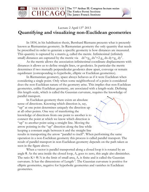
In Euclidean geometry there exists an absolute
sense of directions. Knowing which direction is, say,
“up” at one point determines uniquely the direction up
at all other points. One way of transferring the
knowledge of directions from one point to another is to
connect the point at which we know which direction is
“up” to another point using a straight line. Moving the
arrow pointing in the “up” direction along the line while
keeping a constant angle between it and the straight line
results in transporting the arrow “parallel to itself”. When performing the same
operation in a non-Euclidean geometry this process is called parallel transport. The
result of parallel transport in non-Euclidean geometry depends on the path taken as
seen in the figure above.
When a vector is parallel transported along a closed loop it is rotated by an
angle θ. As the area inside the closed loop, A, goes to zero, this angle also diminishes.
The ratio K= θ/A in the limit of small area, A, is finite and is called the Gaussian
curvature. It has the dimensions of Length -2 . The Gaussian curvature is positive for
elliptic geometries, negative for hyperbolic geometries and vanishes in Euclidean
geometries.

The two dimensional surface of a sphere, together with the notions of lengths
endowed from the ambient three dimensional Euclidean space, give rise to an elliptic
geometry. In general we can realize the lengths prescribed by a given two-dimensional
metric as a surface. The surface is called an isometric embedding of the metric, or a
realization of the metric. For a given geometry there might be many different
realizations as surfaces.
A quantity called the second fundamental form describes how curved a given
surface is. At every point on the surface and at every direction we may fit the surface
with a circle or radius R (directed along that direction), whose center lies on the
normal to the surface. The k=1/R is called the normal curvature along that direction.
The principal curvatures, k 1 and k 2, are the maximal and minimal values of the normal
curvature. Their values describe how curved a surface is. If both curvatures share the
same sign their circles lie on the same side of the surface and the surface is “bowllike”
at that point. If the curvatures have opposite signs the surface they describe is
saddle like. A remarkable result, which goes by the name “Gauss’ theorema
egregium”, states that the product of the two principal curvatures is no other than the
Gaussian curvature, which can be determined from the metric alone, k 1k 2=K. This
implies that there is a close relation between the metric of a surface and the shapes
that surfaces realizing this metric may assume in space.
There are two ways of trying to visualize
non-Euclidean geometry. The first is to assign a
non-Euclidean metric to a given domain, and
examine how straight lines behave. Poincare’s
disk model (which in fact is due to Beltrami) is
such an example. A specific hyperbolic metric is
prescribed on a disk. Straight lines are diameters
in the disk and circle segments that meet the
disk’s boundary perpendicularly. Line segments near the boundary correspond to
longer lengths then the segments situated closer to the center of the disc. In the image
to the right the Poincare disk is plotted along with some geodesics. This model
underlies Escher’s series of wood-cuts named the circle limits. Above we show circle
limit IV.
The other way of making sense of non-Euclidean
geometry is to realize the geometry by a surface. The
paper cuts from last week, which essentially use the
prescription of geodesic curvature to generate a desired
geometry, are such an example. The mathematician Daina
Taimina provided us with a more elegant (and durable)
example by crocheting a disk with hyperbolic geometry.