Real Space Renormalization in Statistical Mechanics

Real Space Renormalization in Statistical Mechanics
Efi Efrati, 1, ∗ Zhe Wang, 1 Amy Kolan, 1, 2 1, 3
and Leo P. Kadanoff
1
James Franck Institute,
The University of Chicago. 929 E. 57 st,
Chicago, IL 60637,
USA
2
St. Olaf College, Northfield, MN,
USA
3 The Perimeter Institute,
Waterloo, Ontario,
Canada
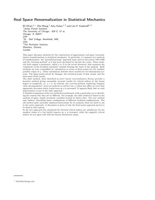
This paper discusses methods for the construction of approximate real space renormalization
transformations in statistical mechanics. In particular, it compares two methods
of transformation: the “potential-moving” approach most used in the period 1975-1980
and the “rewiring method” as it has been developed in the last five years. These methods
both employ a parameter, called χ or D in the recent literature, that measures the
complexity of the localized stochastic variable forming the basis of the analysis. Both
methods are here exemplified by calculations in terms of fixed points for the smallest
possible values of χ. These calculations describe three models for two-dimensional systems:
The Ising model solved by Onsager, the tricritical point of that model, and the
three-state Potts model.
The older method, often described as lower bound renormalization theory, provides a
heuristic method giving reasonably accurate results for critical indices at the lowest
degree of complexity, i.e. χ = 2. In contrast, the rewiring method, employing “singular
value decomposition”, does not perform as well for low χ values but offers an error that
apparently decreases slowly toward zero as χ is increased. It appears likely that no such
improvement occurs in the older approach.
A detailed comparison of the two methods is performed, with a particular eye to describing
the reasons why they are so different. For example, the older method is based on the
analysis of spins, simple stochastic variables located at lattice sites. The new method
uses “indices” describing linear combinations of different localized configurations. The
old method quite naturally employed fixed points for its analysis; these are hard to use
in the newer approach. A discussion is given of why the fixed point approach proves to
be hard in this context.
In the new approach the calculated the thermal critical indices are satisfactory for the
smallest values of χ but hardly improve as χ is increased, while the magnetic critical
indices do not agree well with the known theoretical values.
∗ efrati@uchicago.edu

CONTENTS
I. Introduction 2
A. History: the conceptual foundations 2
B. Statistical Variables 3
C. Renormalization 3
D. Fixed Point 4
E. Critical indices 4
F. Response analysis 4
G. Requirements on approximations 5
H. History of real-space methods 5
I. Comparisons 6
1. Stochastic variables 6
2. Geometric structure 6
3. Calculational strategy 7
J. Plan of paper 7
II. The renormalization process 7
A. Overview 7
1. Introducing new statistical variables 7
2. Tracing out the original statistical variable 8
3. Obtaining a recursion relation 8
B. Basic Statistical Description 9
C. Tensor-SVD Renormalization 11
1. Singular Value Decomposition 11
2. SVD as an approximation method 11
3. Gauge invariance and interpretation of fixed-point
tensor components 12
D. Null space of the response matrix 13
1. Errors 13
E. Lower bound variational renormalization 13
1. Decoration 13
2. potential moving theorem 14
3. Using potential moving 14
4. Spatial vectors and tensors 15
III. Results 15
A. Results from block spin calculations 15
1. Block spin renormalization of Ising models 16
2. Block spin renormalization for other models 17
B. SVD Results 17
1. Generation of SVD fixed point 17
C. Summary of SVD numerical results 19
1. Hexagonal χ = 2 19
2. Square χ = 2 20
3. Hexagonal χ = 3 20
4. Additional fixed point (hexagonal χ = 3) 20
5. And one more (hexagonal χ = 3) 21
6. Square χ = 3 21
7. Square χ = 4 21
8. Four-state Potts model 21
9. The response matrix in tensor renormalization 21
IV. Discussion 22
A. Error estimates 22
B. Work to be done. 23
C. Where do we stand? 24
Appendix: Gauge freedom and invariance of the recursion
step in isotropic TRG 24
Proof 24
Acknowledgments 25
References 25
I. INTRODUCTION
A. History: the conceptual foundations
The renormalization group (1–4), provides a theoretical
understanding of singular problems in statistical mechanics
(5), particularly ones involving phase transitions.
There are two main branches of analysis based upon this
method, one involving work in momentum or wave vector
space (6), the other involving so- called “real-space”
methods. In this review, we follow the latter approach.
Both approaches make extensive use of the following
conceptual ideas, vis
• Scale invariance. Singularities in statistical mechanics
tend to be connected with behaviors that
are the same at different length scales. Critical
points of phase transitions have correlations at all
length scales.
• Scale covariance. Near the phase transition, many
physical quantities vary as powers of characteristic
lengths that describe the system, or of lengths
describing the quantities themselves, or as powers
of “fields” that measure the deviation of thermodynamic
quantities from criticality. These powers
characterize the phase transition. They are called
critical indices.
• Fixed point. The scale-invariance is described by
a Hamiltonian or free-energy-function that has elements
that are independent of length scale. As
a result, one might expect that, for example, the
Hamiltonian or the free energy function that describes
the system will not change when the length
scale changes. This unchanging behavior is described
as “being at a fixed point”.
• Renormalization. A transformation that describes
the results of changes in the length scale. Usually
this transformation will not change the Hamiltonian
or free energy describing the fixed point. That
is the reason for the name, fixed point.
• Universality. Near the phase transition, many different
physical systems show identical behavior of
the quantities that describe critical behavior. Since
these quantities are descriptive of scale-invariant
behavior these descriptive quantities all can be seen
at large length scales.
• Universality classes. There are many critical points
with a wide variety of different origins. Nonetheless
these fall into relatively few universality classes,
each class being fully descriptive of all the details
of a given critical behavior.
The behavior of different critical systems can be, in large
measure, classified by describing the dimension and other
2

topological features of the system, and then describing
some underlying symmetry that plays a major role at
the critical point. Thus, the model that Lars Onsager
solved, the Ising model, (7–9) is mostly described by saying
it is a two-dimensional system with a spin at each
point. The spin can point in one of two directions. The
model has a symmetry under flipping the sign of a spin,
so that it can describe a magnetic phase transition. It
is equally well descriptive of a two-dimensional liquid in
which the basic symmetry is in the interchange of high
density regions with low density ones, so that it describes
a liquid-gas phase transition. Any model with the appropriate
symmetry and dimensionality and the right range
of interaction strengths is likely to describe both situations,
and many others. The Ising model constitutes the
simplest model of this kind.
B. Statistical Variables
There are many models and real systems that exhibit
critical behavior (10–13). All of those with short-range
interactions and spatial homogeneity have the same kind
of characteristic behavior. One starts from a statistical
ensemble, that is a very large system of stochastic
variables, called {σr}, where r defines a position in
space. The statistical calculation is defined by probability
distribution, given as an expression of the form
exp (−βH{σr}), where β is the inverse temperature and
H is the Hamiltonian for the statistical system. One then
uses a sum over all the stochastic variables, defined by
the linear operation denoted as trace, to define a thermodynamic
quantity the free energy, F , as
e −βF
−βH{σr}
= Tr {σr} e . (1a)
Eq. (1a) gives the problem formulation for statistical
physics introduced by Boltzmann and Gibbs and directly
used for renormalization calculations through the 1980s.
In recent years, a slightly different formulation has taken
hold. Since the Hamiltonian is most often a sum of terms,
each containing a few spatially-neighboring σr values, one
can write the free energy as a sum of products of blocks:
e −βF
= trace {σr} BLOCKR, (1b)
each block depending on a few statistical variables. This
formulation applies equally well to the older and the new
formulations of the statistical mechanics. Lately, statistical
scientists have realized the advantage of a particular
special form of writing the product of blocks, called
the tensor network representation. In this representation,
similarly to vertex models, the statistical Boltzman
weights are associated with vertices (rather than bonds)
(14).
R
The tensor network representation describes the connectivity
and interdependence of blocks and statistical
variables. Because of locality the numerical value each
block attains depends on a small number of statistical
variables. Every statistical variable in turn affects the
numerical values in a small number of different blocks.
This allows the identification of a statistical variable assuming
χ different values with an index assuming the
values {1, 2, · · · , χ}. The blocks are linked because each
index appears in precisely two blocks. The blocks then
reduce to tensors whose rank is determined by how many
different indices determine the values assumed by a given
block. Every configuration corresponds to a specific
choice of indices. It is believed, but not proven, that
this kind of representation forms a link to the fundamental
description of the statistical problem (15). The free
energy calculation which follows by summation over all
possible configurations of the statistical variables reduces
to a tensor product tracing out all the mutual index values.
e −βF = Tri,j,k,···
Tijkl
3
(1c)
The tensor indices are indirect representations of the
original statistical variables. Each value of a given index
may represent a sum, with coefficients that can be
positive or negative, of the weights of statistical configurations
in the system. Moreover, this representation
permits a kind of gauge invariance for each index at each
point in space, giving the index variable a new meaning.
For example, if the index i appears in two tensors T 1 ijkl
and T 2 ipqr , then the index transformation,
T 1 ijkl →
m
Oi,mT 1 mjkl, T 2 ipqr →
Oi,mT 2 mpqr, (2)
for
m Oi,mOj,m = δi,j, will leave the partition function
unchanged. This important formal property underpins
the newer statistical calculations.
C. Renormalization
The basic theory describing this kind of behavior was
derived by Wilson (16), based in part upon ideas derived
earlier (17–23). The first element of the theory is the
concept of a renormalization transformation. This is a
change in the description of an ensemble of statistical systems,
obtained by changing the length scale upon which
the system is described. Such a transformation may be
applied to any statistical system, including ones which
are or are not at a critical point. There is a whole collection
of methods for constructing such renormalization
transformations and describing their properties. This paper
will be concerned with describing one class of such
transformations, the real-space transformations. These
are ones that employ the description of the ensemble in
m

ordinary space (or sometimes space-time) to construct a
description of the renormalization process.
The ensemble is parameterized by a set of coupling constants,
K = {Kj}. These couplings might describe the
spin interactions of the early renormalization schemes,
with the subscripts denoting couplings to different combinations
of spin operators. Alternatively the K’s may
be parameters that determine the tensors. The renormalization
transformation increases some characteristic
distance describing the system, usually the distance between
neighboring lattice points on a lattice defining the
spatial structure, so that this distance changes according
to a ′ = δL a. Correspondingly, the renormalization
transformation changes the coupling parameters to new
values which we denote by K ′ . These new couplings depend
upon the values of the old ones, so that
K ′ = R(K) (3)
Here, the function R represents the effect of the renormalization
transformation.
D. Fixed Point
The renormalization theory is particularly powerful at
the critical point. This application of the theory is based
upon the concept of a fixed point, an ensemble of statistical
systems that describe the behavior of all individual
statistical systems within a particular universality class.
Since the critical point is itself invariant under scaling
transformations, the ensemble in question is invariant under
a renormalization transformation. It is said to be at
a fixed point. The fixed point is represented by a special
set of couplings, K ∗ , that are invariant under the
renormalization transformation
E. Critical indices
K ∗ = R(K ∗ ) (4)
The most important physical effects are obtained by
studying the behavior of the renormalization transformation
in the vicinity of the critical points. This behavior
is in turn best described by a set of critical indices
describing the scaling of the singular part of measurable
physical quantities near the critical point. One writes the
deviation of the Hamiltonian from its fixed point value
as
−βH = −βH ∗ +
hα S α
(5)
where the components hα represent the small deviations
of the coupling constant Kα from their fixed point values,
while S α are the extensive stochastic operator conjugates
α
to the Kα. The free energy undergoes a change in value
produced by these variations of the form:
−βδF =
CαηαL d−xα
(6)
α
Here, the ηα describes linear combinations of the hj, each
ηα defining a different kind of covariant scaling operator
that describes a particular type of scaling near the critical
point. In the usual critical phenomena problems one
such operator describes the field thermodynamically conjugate
to the order parameter whose symmetry breaking
produces the phase transition, and another such field,
conjugate to the energy density, is the deviation of temperature
from its critical value. Still other operators,
such as the stress tensors, play important roles in the
critical behavior, but have symmetries that prevent them
from appearing at first order in this expansion.
In Eq. (6), L is the linear dimension of the system,
d is the dimensionality of the system, while Cα is a relatively
unimportant expansion coefficient. The crucial
quantity in this equation is x α , the critical index defining
the scaling properties of the scaling operator. For the
usual always-finite scaling operators the exponents x α are
positive. Operators for which the corresponding critical
exponents lie between zero and the dimension of the system,
d, are called relevant operators. These play a major
role in the thermodynamics. Operators for which the
corresponding critical exponents are greater than d are
called irrelevant operators and do not contribute to the
to the singular behavior of the thermodynamic functions
(24; 25). In our work below, we shall compare the values
of the relevant x’s as they emerge from the approximate
numerical renormalization theory with the exact values
that are often known from other numerical work or exact
theories (26; 27).
F. Response analysis
The behavior of the renormalization transformation in
the vicinity of the critical points is quantified by the response
matrix relating small changes in the couplings,
Kj, with the small changes they induce in the renormal-
ized couplings , K ′ i .
dKj
Bi j = dK′ i
K=K∗ 4
. (7)
This matrix has right and left eigenfunctions defined as
Bi j ψj α = E α ψi α
and
φα i Bi j = E α φα j
(8)
j
The eigenvalues define the scaling properties of the exact
solution. The operators’ scaling is defined by Eq. (6).
The eigenvalues directly determine this scaling since
E α = (δL) yα
= (δL) d−xα
i
(9)

with δL being the change in length scale produced by
the renormalization. 1 Different authors describe their
results in terms of Eα, or y α , or x α . In this paper, we
use the last descriptor.
The eigenfunctions φ and ψ can be used to construct a
set of densities, o α (r), of operators called scaling operators
since they have simple properties under scale transformations.
The combinations
j
s j (r)ψj α = o α (r) (10a)
define o α (r) as the densities for the scaling operator.
These operators and their extensive counterparts O α =
r oα (r) respectively scale like distances to the power
−xα and yα respectively. The other coefficient in the
eigenvalue analysis, φa i can be interpreted by saying that
s i generates a combination of fundamental operators according
to
s i (r) =
α
φα i o α (r) (10b)
To make Eq. (10a) and Eq. (10b) work together, we
must define the eigenvectors so that they are normalized
and complete
i
φα i ψi β = δα β
and
G. Requirements on approximations
α
φα j ψi α = δi j
(11)
The concepts of renormalization and scale invariance
lead naturally to the identification of scaling and universality
and have contributed to the fundamental understanding
of critical phenomena. There is also a more
practical aspect of the renormalization concepts that allows
one to predict the location of phase transitions of
specific systems and describe their nature in terms of the
critical exponents. However, for most systems, carrying
out the actual renormalization cannot be done exactly.
Instead, some approximation method must be used to
find an approximate renormalization transformation. We
hope that the approximation method might give an informative
picture of the physical system, that it might be
numerically accurate, and that it might be improvable so
that more work can lead to better results.
1 If δL1 and δL2 are two rescaling factors, then the form of
the eigenvectors as a function of these rescaling factors satisfy
E(δL1 · δL2) = E(δL1)E(δL2). It follows that E(1) = 1
and that E ′ (δL1)/E(δL1) = C for some constant C, leading to
E(δL) ∝ δL y (28).
H. History of real-space methods
The first heuristic definition of a real space renormalization
was given in (20). After Wilson and Fisher
(6; 29) demonstrated the viability of the renormalization
approach by inventing the ɛ expansion, Neimeijer and
Van Leeuwen (30; 31) described a method for doing a
numerical calculation of the renormalization function, R,
in terms of a small number of different couplings. These
methods were then described in one dimension (32) and
applied (33). From the point of view of this paper, an important
advance occurred when a variational method was
invented (34) and extensively employed (33; 35–42). This
method was described as a lower bound calculation since
it permitted calculations that gave a lower bound on possible
values of the free energy. This approach permitted
reasonably accurate and extensive calculations of critical
properties in two and higher dimensions. However, as
the 1970s came to an end, the lower bound method fell
into disuse.
In part, the disuse arose because interest turned from
problems in classical statistical mechanics to quantum
problems. Although path-integral methods permit one
to convert a quantum problem into one in classical statistical
mechanics, the lower bound method seemed to work
best when the problem had the full rotational symmetry
of its lattice, and hence did not apply to many quantum
problems. In 1992 White (43) invented a quantum mechanical
real space renormalization scheme that worked
beautifully for finding the properties of one dimensional
quantum systems via numerical analysis. This success
started a large school of work aimed at these problems
and analogous problems in higher dimensions (44–47).
White’s method looked very different from the realspace
work of the 1970’s. It did, however, have an important
provenance in Wilson’s numerical solution of the
Kondo problem (48). White studied the approximate
eigenstates involving long chains of correlated spins, and
how those long chains interacted with small blocks of
spins. There was also earlier work that focused on blocks
of a small number of spins. In the course of time, connections
among the different approaches began to be appreciated.
As pointed out by, for example, Cirac and
Verstraete (49), the correlations within wave functions
were produced by summing products of correlations on
small blocks, producing situations described as “tensor
product states”. Levin and Nave (50), Gu and Wen(51),
and Vidal and coworkers(46; 47) described how an accurate
analysis could be constructed based on the correlations
among statistical variables located at a very small
number of nearby lattice sites.
On the one-dimensional lattice, Vidal (46) and coworkers
use two or three neighboring lattice sites as the basis
of the correlations. In higher dimensions Levin and Nave
use a hexagonal construction in which the basic variables
are three tensor indices, each independently taking on in-
5

teger values grouped around a three-legged lattice site.
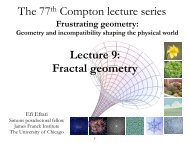
Gu and Wen correspondingly use a four index tensor describing
the intersections in a square lattice (see Figure
(1)) .
i j
l
k
i j
T
FIG. 1 The basic tensor network used here for the SVD renormalization
calculations. Tensors are represented by blue solid
colored squares. Red circles denote the position of the tensor’s
indices. Every tensor has four indices. Every index assume
integer values between one and χ, and is shared between exactly
two tensors. Four indices determine the configuration
of the statistical variable, and the corresponding tensor entry
gives the statistical weight of the configuration. Note that
the interactions represented by the tensors occupy half the
available space. The left inset shows the labeling of the indices;
the right inset shows the same tensor in the stick-figure
usually used in the literature.
I. Comparisons
The main points of difference between the work of the
1970s and that of the last two decades include
1. Stochastic variables
We have already mentioned that the 1975 scheme uses
spins while the recent scheme employs much more complex
spatial structures labeled by tensor indices. Both
approaches need to reflect the underlying symmetry of
the problem at hand, for example the spin flip symmetry
of an Ising model. The early work used spin variables
that directly reflected the symmetry. 2 In contrast, the
2 However, there were occasional uses of more complex variables.
In Burkhardt’s(35) Ising model calculation, the “spin” variable
could take on three values: ±1 and zero. The last value reflecting
a hole unoccupied by a magnetic spin.
l
k
more recent work has replaced summation over spin variables
by sums over tensor indices. The basic symmetries
are hidden in the structure of these tensors. In using
this tensor representation, recent workers have used universality
to say that they can use any problem-definition
that reflects a desired symmetry. They then also argue
that the proper meaning of the tensor indices will give
them direct access to the deep structure of the statistical
mechanics problem (52).
Each tensor index can take on χ possible values, representing
that number of different configurations of the system.
Recent workers believe, but have not proven, that
they can get perfect accuracy when χ is infinite. Consequently
they reach for approximation methods that permit
them to increase χ until it reaches quite large values.
( Note that these indices with their large number of possible
values can simultaneously approximately represent
many kinds of different variables: many-component vectors,
Ising spins, or continuous variables. ) In contrast
the earlier workers felt that arbitrary accuracy would not
be available to them. The best that was expected was a
qualitatively accurate description of the problem.
We use the term summation variables to describe both
the spins of the earlier work, and the stochastic variables
linked to the tensor indices more recently used.
2. Geometric structure
Another difference can be seen in the geometric structures
used to describe the interactions among the summation
variables. In the tensor work the summation variables,
in a similar fashion to their role in vertex models,
(e.g. see (14)), are associated with bonds and their interactions
are associated with vertices. This constrains each
summation variable to participate in exactly two interactions
(connect two vertices). The interactions, however,
are less constrained and typically group together several
summation variables around a rank m vertex.
In the earlier renormalization work, in contrast, the
summation variables are associated with vertices and
thus may participate in more than two interactions. The
interactions are associated with blocks of summation
variables allowing more than only pairwise interactions.
This difference not only manifests in the formulation of
the partition function of each of the representations but
more importantly restricts the placement of the rescaled
summation variables and their interactions. In the earlier
work new summation variables could be placed arbitrarily
provided the interactions they participate in can
be formulated in term of the old interaction blocks. In
the tensor representation the binary interaction structure
must be preserved when introducing new summation
variables. Thus every introduction of a new summation
variable is necessarily associated with changing the interaction
connectivity of the old variables.
6

3. Calculational strategy
The earlier work found the properties of critical points
via a method based upon the analysis of fixed points.
First, the critical system was brought to a fixed point.
Critical indices were then calculated by looking at the
growth or decay under renormalization of small perturbations
about the fixed point, using a method based upon
eigenvalues (see Sec. (I.F).) The main output of the calculation
were a set of critical indices which could be compared
among calculations and with theoretical results.
In contrast, tensor analysts seldom calculate fixed
points. 3 Instead they calculate free energies and other
thermodynamic quantities by going through a large number
of renormalizations, usually increasing the value of χ
as they go. (As we shall see, it is natural to square the
value of χ in each tensor renormalization.) When they
reach a maximum convenient value of χ they employ approximations
that enable them to continue to renormalize
with fixed χ. These calculations then show the thermodynamic
behavior near criticality.
The non-appearance of fixed points in many of the
tensor calculations provides an important stylistic contrast
between that work and the studies of the 1975-era.
The calculation of fixed points for the critical phenomena
problems permits the direct calculation of critical indices
and thus offers many insights into the physics of the problem.
The insights are obtained by keeping track of and
understanding every coupling constant used in the analysis.
This is easy when there are, as in Ref.(34), sixteen
couplings. However, the more recent tensor-style work
often employs indices which are summed over hundreds
of values, each representing a sum of configurations of
multiple spin-like variables. All these indices are generated
and picked by the computer. The analyst does not
and cannot keep track of the meaning of all these variables.
Therefore, even if a fixed point were generated,
it would not be very meaningful to the analyst. In fact,
the literature does not seem to contain much information
about the values and consequences of fixed points for the
new style of renormalization.
The fixed point method seems more fundamental and
preferable, but offers major challenges when the value of
χ is large.
3 Notable exceptions include the Hamiltonian work of Vidal and
coworkers (46; 47), in which a fixed point Hamiltonian is indeed
calculated. For statistical rather than quantum problems, fixed
point studies were done by Ref.(53) and Ref.(54). This fixed
point analyses, however, were only be carried out for small values
of χ.
J. Plan of paper
The next section describes the block spin and the
rewiring methods employing singular value decomposition
(SVD) used for renormalization by Ref.(50) and
Ref.(51). Sec. (III) outlines the results from these calculations,
including some new results for both the 1975
method and also the rewiring calculations. The final section
suggests further work.
II. THE RENORMALIZATION PROCESS
A. Overview
We now come to compare different approximate real
space renormalization schemes. The starting point for
the considered methods is a system described by the statistical
variables, {σ}, and a Hamiltonian H{σ}. In the
1975 scheme this Hamiltonian is directly used to define
the partition function
Z = Tr {σ}e −βH . (12a)
In the newer scheme, the Hamiltonian is used to define to
define a two-, three-, or four- index tensor along the lines
described in Sec. (II.B) below. The partition function
is then defined as a statistical sum in the form of a sum
over indices of a product of such tensors, in the form
or
two index: Z = Tri,j,k,...,n TijTjk.....Tni (12b)
four index: Z = Tri,j,k,...,
Tijkl
7
(12c)
In both cases, the setup of the tensor product is such
that each index appears exactly twice. In this way, the
system can maintain its gauge invariance as an invariance
under the rotation of each individual index. We can then
imagine that these partition functions may equally well
be described in terms of the values of coupling constants,
K, or of the value of tensors, T .
Working from this starting point, the renormalization
scheme is implemented through three steps as follows:
1. Introducing new statistical variables
In the 1975-style scheme, the new variables are defined
to be exactly similar to the old variables, {σ}, except
that the new variables are spaced over larger distances
than the old ones (See Figure (2).) 4 . A new Hamiltonian
depending on both old and new variables, is defined
4 In fact, this identity of old and new is one of the major limitations
of the older scheme.

y adding to the old Hamiltonian an interaction term 5 .
˜V ({µ}, {σ}). This term is defined so that the partition
function remains unchanged by the inclusion of the µ’s.
This invariance is enforced by the condition
Tr {µ} e −β ˜ V ({µ},{σ}) = 1 (13a)
so that the partition function can be written as
Z = Tr {σ}e −βH({σ)} = Tr {σ}Tr {µ}e −βH({σ)}−β ˜ V ({µ},{σ}) .
(13b)
A roughly similar analysis can be used in the tensor network
scheme. Starting from the definition of the partition
function as the trace of a product of tensors in Eq. (12c)
one replaces each of the rank four tensors by a product
of rank three tensors, using a scheme derived from the
singular value decomposition (SVD) theorem (See Sec.
(II.C.1) below.) as 6
Tijkl = Trα UijαVklα
leaving us with
Z = Trijkl... Tmnpq = Trijkl... Trαβγ...
2. Tracing out the original statistical variable
(14a)
UijαVklα
(14b)
In the 1975 scheme the trace over the original statistical
variables, {σ}, defines a new Hamiltonian H ′ which
depends solely on the new variables {µ},
so that
e −βH′ {µ} = Tr{σ}e −β ˜ H({µ},{σ})
Z = Tr {µ}e −βH′ {µ}
(15)
(16)
One can expect that some approximation will be needed
in order to calculate the sum over the σ’s.
A roughly analogous procedure can be applied to the
tensor sums in Eq. (14). If the position of the UV products
and the new indices have been deftly chosen, the old
indices will appear in a series of small islands in which
each island is only coupled to a limited number of new
indices. Following Ref.(51), we shall work with the case
5 The˜appears on this V to distinguish it from another use of the
symbol V , that is the V that conventionally appears in singularvalue-decomposition
analysis.
6 The standard SVD scheme produces a matrix-multiplication
product. T = UΣV T r where Σ is a diagonal matrix. The diagonal
entries in Σ are non-negative and are called singular values.
In the notation in Eq. (14a) the Σ is absorbed into the U and
V .
in which that number is four. After a rearrangement, the
partition function sum in Eq. (14) may be written as
Z = Trαβγ...Trijklmn... U(ij, α)V (α, kl) ( Tmnpq)
The sum over the old tensor indices may then be performed,
generating new tensors, T ′ αβγδ , so that
3. Obtaining a recursion relation
Z = Trαβγ... ( T ′ αβγδ) (17)
The new degrees of freedom, µ, have been defined to be
identical to the variables, σ, the only difference being that
the µ’s are defined on a rescaled system. This identity
usually permits the extraction of new coupling constants,
K ′ from the new Hamiltonian. The new couplings are
then connected to the old via the recursion relation K ′ =
R(K).
If the recursion relation is calculated exactly, the new
set of couplings will likely contain many more terms than
the old set. This proliferation of couplings reflects the
additional information from several blocks of the old system
that we are trying to cram into one block of the new
one. An approximation is needed to limit the new couplings.
This limitation usually results in a situation in
which the possible couplings include only those that can
be formed from spins completely within a geometrically
defined block. Couplings which include spins from several
blocks are excluded. One example of such a block is
shown in Figure (2).
The tensor scheme has a different approach. In order
to do renormalizations, the new partition function calculation
of Eq. (17) must have the same structure is the
old one in Eq. (12c). As we discuss in detail in Sec.
(II.C.1) below, this structural identity is violated by the
exact theory in which there are many more new indices
than old. To obtain a recursion relation, one must use an
approximation to eliminate the proliferation in the summation
degree, χ. As we shall discuss in Sec. (II.C.1)
below, an approximation of this kind is automatically
provided by the SVD method. Using this approximation
method, one has a renormalized problem with exactly
the same structure as the original problem. The result
may be expressed as a recursion relation for the rank four
tensor
T ′ = S(T ) (18)
or as a recursion relation for the parameters defining
those T ’s, e.g. K ′ = R(K).
There is a difficulty in using tensor components in the
recursion relation of Eq. (18). Because of the gauge
invariance the components of the new tensor, T ′ are not
uniquely defined. To ensure uniqueness, it might well be
better to define the tensors in terms of gauge invariant
8

decoration
summation
potential moving
FIG. 2 The setup for a potential moving scheme on a square lattice. The old spins (σ) are marked by filled black circles located
at the vertices of a square lattice. Note that each such spin belongs to four different squares. These squares form the “blocks”
for our calculation. The new spins, µ appear in one quarter of the blocks, and are marked as filled bright red circles. The (red)
lines emanating from these new spins denote coupling terms that link these to the old spins. Each such coupling connects a
single old spin to a new one. The potential moving places all the interactions between old spin in blue squares. The old spins
around every blue square are connected only to themselves and to new spin variables. They can be summed over, giving a new
effective coupling between adjacent new spins.
parameters. While this may be done relatively easily
for low χ values, identifying all the independent gauge
invariants for high χ value tensors may be a daunting
task.
With a recursion relation at hand one may apply all
the tools described in the previous section and obtain a
fixed point Hamiltonian and the corresponding critical
exponents.
In the remainder of this chapter, we describe the nuts
and bolts of the real space renormalization process, using
as our example square lattice calculations based on Isingmodels
and the version of tensor renormalization found in
(51). We particularly focus on understanding the differences
between the older (34) and the newer styles (50; 51)
of doing renormalization work.
B. Basic Statistical Description
In Sec. (I.I.1) we pointed out that the older calculations
are based upon summations over defined stochastic
variables like the Ising models σr = ±1. These
calculations then use a Hamiltonian H({σ}) to define
the statistical weight of each configuration of the variables.
Consider a problem involving four spin variables,
σ1, σ2, σ3, σ4, sitting at the corners of a square (see Figure
(3)), each variable taking on the values ±1. If this problem
has the symmetry of a square, it can be described in
terms of the following combinations
S0 = 1,
S1 = σ1 + σ2 + σ3 + σ4,
Snn = σ1σ2 + σ2σ3 + σ3σ4 + σ4σ1,
Snnn = σ1σ3 + σ2σ4,
S3 = σ1σ2σ3 + σ2σ3σ4 + σ3σ4σ1 + σ4σ1σ2,
S4 = σ1σ2σ3σ4. (19)
The spin combination variables Si form a closed algebra,
i.e. any function of the spin variables of Eq. (19)
may be expressed as a linear sum of these same variables
with constant coefficients:
F (S0, S1, Snn, Snnn, S3, S4) = aiSi .
9

2
3
FIG. 3 Identification of the spin variables located at the vertices
of a square unit cell.
One important example of this set of variables, denoted
as [S] is a Hamiltonian H sq [S] which describes the most
general isotropic interactions with the symmetries of a
square unit block that can be formed from the set of
σi’s . The basic block used in the 1975 renormalization
calculation is given in terms of this Hamiltonian as
BLOCK = e −βHsq [S] with −βH sq [S] =
1
4
i
KiSi (20)
Here the K’s are called coupling constants and their values
provide a numerical description of the problems at
hand.
In contrast, a whole host of new calculations replace
the coupling constants by tensors, and use the tensor
indices as a proxy for statistical variables. To illustrate
this process, we write the tensor, Tijkl, for the cases in
which each index can take on two possible values and in
which there is once more the symmetry of a square. The
tensors are situated on every other square and therefore
capture only half of the possible four spin interaction
and next nearest neighbor interaction. 7 We use the spin
notation to write the tensor as
T = e KiSi . (21)
There is considerable flexibility in defining the indices 8 .
For example, we could let one index-value, (+), correspond
to positive spin and the other, (-), to negative
spin. Then the tensor components would have the following
distinct values
7 We note that allowing the index four possible values allows the
description of every interaction in Eq. (19). However, in favor
of simplicity we restrict our present treatment to the two valued
index tensors only.
8 In fact that flexibility is a sort of freedom under gauge transformations,
and that freedom represents one of the main attractions
of the tensor approach.
10
T++++ = exp(K0 + 4K1 + 4Knn + 2Knnn + 4K3 + K4),
T {+++−} = exp(K0 + 2K1 − 2K3 − K4),
T {++−−} = exp(K0 − 2Knnn + K4),
T {+−+−} = exp(K0 − 4Knn + 2Knnn + K4),
T {+−−−} = exp(K0 − 2K1 + 2K3 − K4),
T−−−− = exp(K0 − 4K1 + 4Knn + 2Knnn − 4K3 + K4),
(22)
where curly brackets stand for all cyclic index transformation,
i.e.
T {+++−} = T {++−+} = T {+−++} = T {−+++}.
Alternatively, one might use the index values i = [1] to
represent a sum over the statistical weights produced by
the possible spin configuration (σ = +1) and (σ = −1)
and the index [2] to represent a difference between these
two statistical weights, specifically
[1] =
(+) + (−)
√ 2
and [2] =
(+) − (−)
√ 2
(23)
The factor of √ 2 is introduced to make the index-change
into an orthogonal transformation. Under this definition
the tensor-representation would also have six distinct
components however their values in the different
representations change according to
˜Tijkl = OimOjnOkoOlpTnmop, (24)
where O denotes the orthogonal transformation which
maps the indices +− on the right to the new indices [1]
and [2] that appear on the left. For example:
˜T1111 = 1
4
˜T {1112} = 1
4
T++++ + 4T+++− + 4T++−−
+ 2T+−+− + 4T+−−−− + T−−−− ,
T++++ + 2T+++− − 2T+−−−− − T−−−− .
It is important to note that Eq. (24) gives two different
descriptions of the very same tensor, T , in different
bases systems. The tensors remain the same, but the
coordinate system is varied.
Of course, the case described here is rather simple. The
renormalization transformation develops, at each step, a
succession of tensors, usually of increasing complexity,
At each step, the partition function depends upon the
tensor in question, but is independent of the particular
representation of that tensor. When applied successively
to the redefinition of indices in each step of a long calculation,
the index method provides a flexibility and power
not easily available through the direct manipulation of
spin-like variables. We shall see this flexibility in the
specific calculations of renormalizations to be described
in Sec. (III) of this paper.

C. Tensor-SVD Renormalization
In this section, we complete the discussion of renormalization
as it was set up by Ref.(50) and Ref.(51) and then
carried out by Ref.(53) and Ref.(54). We begin with introducing
the main tool of the method, the singular value
decomposition, and discuss its properties. We then discuss
the underlying geometry of the tensor network and
review the tensor gauge freedom.
1. Singular Value Decomposition
The new renormalization methods described in this paper
are based upon the papers of Ref.(50) and Ref.(51).
(See also, for example (44; 55)). These make use of the
singular value decomposition theorem in their analysis.
The theorem states that every real matrix Mij can be expressed
as a product of a real unitary matrix, a diagonal
non-negative matrix and another real unitary matrix:
Mij =
ΨαiΛαΦαj, (25)
α
where
α ΨαiΨαj = δij and
α ΦαiΦαj = δij. While
the decomposition is not unique the non-negative real
numbers, Λα are unique. Customarily, the Λ’s, called
singular values, appear in descending order. When so
ordered Eq. (25) with only the χ largest components of
Λ taken into account (the remaining set to zero), yields a
rank χ approximation of M which is optimal in the least
square sense. 9 When χ = n, the SVD approximation of
Eq. (25) is exact.
For the specific case of a square n by n real matrix we
may identify
Φαj = φαj, Λα = |Eα|, and Ψαj = sign(Eα)ψαj,
where as above the φ and ψ vectors denote the left and
right eigenvectors of M satisfying
Mij =
n
ψαiEαφαj. (26)
α=1
Finally, we may fold the singular value into the matrices
Φ and Ψ:
Uαi = Ψαi|Eα| 1/2 and Vαj = Φαj|Eα| 1/2 . (27a)
9 More precisely, the SVD estimate of M, called M χ , serves serves
to minimize the quantity Q = trace(M − N) 2 within the class
N’s that are matrices with only χ non-zero eigenvalues. The
minimizer is given by N = M χ .
The above matrices allow us to rewrite the rank χ approximation
of M as a product:
Mij ≈ M χ ij = Σ χ
α=1 UαiVαj
11
(27b)
This approximation will be used throughout the discussion
of rewiring methods. Notice that the approximation
in Eq. (27) becomes exact when χ = n. Also, the
above decomposition of Eq. (27b) is not unique. As the
columns of Ψ are the normalized eigenvectors of MM T ,
they have a sign ambiguity. One may lift this ambiguity,
as we do in our following calculations, by setting the
sign such that the first non-vanishing component of each
eigenvector is positive. Note, however, that this resolution
of the sign ambiguity is not invariant under a base
change.
2. SVD as an approximation method
For a square lattice, one writes down the tensor product
representation of the partition function as the trace
over a product of rank four tensors
Z = Trijklmn...
Tijkl,
in which each index occurs precisely twice. The summation
depends strongly on the topology of the network
comprised of the indices connecting adjacent tensors. For
this reason the usual methods of describing tensor calculations
make heavy use of pictures. We shall follow that
precedent.
We show the tensor lattice in Figure (1). Each colored
box is a four-legged tensor. The tensor indices appear at
the corners as filled circles. The inset shows the definition
of these indices. The task at hand is to introduce new
indices while isolating small groups of old indices so that
these groups make no contact with other old indices. To
do this we rewrite a potential term like Tijkl as a matrix
product in the form
T approx ijkl =
χ ′
α=1
UijαVklα
(28)
where α is the new index. There are six ways of doing
this, involving different placements of the indices ijkl in
U and V . Two of these are depicted in Figure (4).
The singular value decomposition theorem points out
that we can make Eq. (28) give an exact expression for
the four-legged tensor by using SVD and letting χ ′ = χ 2 .
Alternatively we may use a smaller value of χ ′ , as for
example χ ′ = χ, and use either SVD or some other
method to get a good approximation involving U and
V . This kind of replacement is called a rewiring because
it changes the connections in our lattice. The change suggested
by Gu and Wen(51) is shown in Figure (4). This

such an interpretation is not necessary as fixed point
analysis is not performed. Instead only the value of the
partition function (and from it the value of free energy) is
calculated as a function of a varying parameter, say the
temperature. For a fixed point analysis, as we present
here, one may wish to be able to cast meaning to the
components of the fixed point tensor, and through them
to the critical exponents.
D. Null space of the response matrix
The gauge symmetry discussed above implies the existence
of a null space for the response function whose
dimension is at least χ(χ−1)/2. Most of the works which
analyze fixed point tensors employ gauge fixing by treating
a specific subset of the possible tensors. In these
theories the number of independent variables is greatly
reduced, and they don’t display the above null space.
Another contribution to the null space comes from the
loss of information in the the truncation of the SVD decomposition.
The number of independent components in
a χ 2 by χ 2 matrix, in the general case scales as d1 ∝ χ 4 .
If however the χ 2 by χ 2 matrix is known to have only
rank χ then the number of independent components reduces
dramatically and scales as d2 ∝ χ 3 . This implies
a null space of dimension at least d1 − d2 ∝ χ 4 . In the
physical systems symmetries greatly reduce the number
of independent tensor entries, and therefore also reduce
the amount of information lost.
1. Errors
When χ ′ < χ 2 the approximate rewiring will generate
an error. We denote the local error resulting from the
approximation by
Errorijkl = ln[Tijkl/T approx ijkl] (31)
This is the error of a single tensor at a specific configuration
given by its indices values. The SVD scheme yields
an error for the tensor that is optimized in a mean square
sense (50; 51). In the analysis of these authors, the error
term is then simply neglected. This method works exceptionally
well for large values of χ, for which the error
is quite small. In Sec. (III) and Sec. (IV) we shall see
that this strategy does not work exceptionally well for
smaller χ.
An alternative approach to the neglect is to replace
the error term by its maximum (minimum) over tensor
indices. This yields an error of definite sign and in turn
gives a lower (upper) bound on the free energy. This
approach can even be used to find optimal values for U
and V so as to give a best bound for the free energy.
13
The 1975 work employed a one parameter family of
local lower bound approximations. The value of the parameter
was carefully chosen such as to minimize the
global error of the free energy, resulting in an error term
that is quadratic in the local error term. In contrast the
SVD scheme yields a free energy error that is linear in
the error of Eq. (39).
This 1975 method proved to give plausible results for
low χ values. We now turn to a discussion of this method.
E. Lower bound variational renormalization
In this section, we complete the description of the
lower-bound variational method. We first introduce the
local conditions, formulated in terms of the symmetry of
the Hamiltonian, which give rise to a lower bound on the
free energy. We then construct a one dimensional family
of such lower bound potentials characterized by a single
parameter, p. We finally show how to choose the parameter,
p, such as to globally minimize the resulting error
in the free energy.
1. Decoration
As noted in section II.A the first step towards a renormalization
is to introduce new statistical variables to the
system, a process known as decoration. In Eq. (14) we
described the tensor analysis scheme for doing the decoration.
Here we describe in more detail the 1975 scheme
for decoration.
In general each of the new degrees of freedom, which
we will denote by µ, is coupled only to a small subset
of the old spin variables σ through a coupling potential
v([σ], µ), (where [σ] defines the small subset of the old
spin variables). For example, in Figure (2) every new
degree of freedom is placed within an interaction block
an interacts only within this block with its four nearest
neighboring old spin variables. We define a new Hamiltonian
within the interaction block of the new variable
by
˜h([σ], µ) = h([σ]) + v([σ], µ). (32)
where h[σ] is the old Hamiltonian for the block. Choosing
the coupling potential to satisfy
Trµe −βv([σ],µ) = 1, (33)
regardless of the specific value the variables σi, renders
the partition function, and thus the free energy, unchanged
by the inclusion of the new variable. The full
decoration is obtained by using
˜V ({σ}, {µ}) =
v([σ]R, µR)
R

where the sum over R is a sum over all µ-sites. With the
new Hamiltonian being ˜ H = H + ˜ V , the full partition
function is unchanged by the decoration as in Eq. (13).
The 1975 scheme associates one new µ-spin with the
group of four old σ-spins in a surrounding square block.
There are multiple ways to choose a potential interaction
among the spins that will satisfy Eq. (33). Following
(34), and Figure (2) we define a one parameter family of
such potential v p ([σ], µ), where the parameter p serves
to vary the strength of interaction amongst the new and
old spins. This parameter will later allow us to optimize
the choice of potential. The family of potential are given
explicitly by
−βv p ([σ], µ) = pµ(σ1 + σ1 + σ3 + σ4) + c([σ])
= pµS1 − ln(2 cosh(p S1)) (34)
where S1 is defined in (19) and c([σ]) is chosen such that
the sum of e −βv over all values of µ gives unity. Because
of the closed form algebra of the isotropic spin variable
(19) we also know that the constant c(σ) may be rewritten
as a linear function of the isotropic invariant
c([σ]) = aiSi.
As a result, the potential v p (σ, µ) may be written as a
linear combination of the Si values with coefficients which
depend on the variational parameter, p.
2. potential moving theorem
The 1975 paper (34) employed a device for making
the renormalization sum tractable that goes under the
name of potential-moving. This device makes use of the
following theorem: Let us consider the statistical sum
e −βF = Tre −βH where the trace gives a sum over a positive
semi-definite set of terms involving a Hamiltonian
H, giving rise to a “free energy”, F . Now assume that
−βH = −βHa + δV . Here, we shall use Ha to generate
and approximate free energy, F a which we hope will
have a value close to that of the exact free energy, F . Our
calculation makes use of the symmetry of −βH and δV ,
in which we demand that δV be odd under some exact
symmetry of −βH, so that
This condition yields
Tr[e −βH δV ] = 0. (35)
a
−βF
e = Tr e −βHa a
−βF
implies e ≥ e −βF
(36)
To derive Eq. (36) define a Hamiltonian that interpolates
between the exact and the approximate Hamiltonians
and a free energy that arises from this interpolation.
−βH(λ) = −βHa + (1 − λ)δV and e −βF (λ) = Tre −βH(λ)
These definitions imply that
and
d
dλ
βF (λ) =< δV >λ
d 2
(dλ) 2 βF (λ) = −[δV − < δV >λ] 2 λ
14
where the λ subscript means that the average is calculated
using a Hamiltonian H(λ). It follows from Eq. (35)
that the first derivative vanishes at λ = 0. The second
derivative is always negative. Therefore the interpolating
free energy is always larger that the true free energy.
At λ = 1 the interpolating free energy reduces to our
approximate free energy. Consequently,
βF a 1
−βF = − dλ (1−λ) [δV − < δV >λ] 2 λ ≤ 0 (37)
0
Thus, the error in the approximation is of second order
in δV and that the approximate free energy provides an
upper bound for the real free energy.
3. Using potential moving
To construct our approximate renormalization transformation,
we need to make sure that the old spins are
in isolated small groups, each group coupled to the new
spins, but not to any other old spins. If all the couplings
obey this condition we can calculate the new approximate
Hamiltonian.
We start from a situation in which the lattice is divided
into square blocks as in Figure (2). There are
three kinds of blocks. In figurative language, we think
of δV as containing some inconvenient couplings that interfere
with our calculation of the partition function in
Eq. (36). What we do is then “move” the inconvenient
couplings from their inconvenient positions (in the newspin
blocks) to convenient positions in the other blocks.
These convenient positions are required to be completely
equivalent in the exact version of the calculation to the
inconvenient sites so that Eq. (35) may be satisfied. It
is only our motion that produces the distinction between
these two classes of sites.
The geometry of our calculation is shown in Figure
(2). The original Ising spins appear as black dots at the
vertices of the squares. The new variables are the red
dots in the red squares. The new spins are linked to the
old spin variables by interactions indicated by the red
bonds. Those bonds have interactions of the form e pσµ .
All the squares have interactions described by blocks of
the form
BLOCK = exp (−βH sq ) (38)
where the exponent is given by the block Hamiltonian
using the stochastic variables defined by Eq. (19). In

addition the red squares have a potential in the form of
c[σ] as given by Eq. (20).
All the old interactions from the red squares and the
green ones are “moved” into the blue squares. The potentials
that exist at these squares define the motion. They
are
V = −H sq on green squares
V = −H sq + c([σ]) on red squares
V = 3 ∗ H sq − c([σ]) on blue squares (39)
The value of the potential on the blue squares is picked
so that the sum of all the potential terms is zero, allowing
for the double weight of the green squares. The new
interaction between the old and new spins can be formulated
as a pairwise interaction between the new spin µ
and each of its surrounding old spins. It therefore can
be reformulated to be centered about the blues squares
without any approximation. After the motion of the potentials,
we end up with no potential on green or red
squares and a total potential 4 ∗ H sq − c([σ]) on each
blue square.
The error generated by the potential moving is proportional
to the mean variance in the V of Eq. (39).
After that motion the spins at the four vertices of each
blue square are linked to each other and to the surrounding
new spins but to none of the other old spins. This
condition permits summations to be performed over each
blue square independently of all the others, thereby producing
interactions. The result is
e −βH′sq ([µ]) = Tr[σ] exp[ − 4βH ′sq ([σ]) − c([σ])
+ p 4
j=1 (σjµj)] (40)
The new coupling may then be projected out of the new
Hamiltonian. This projection then gives us the recursion
relation.
4. Spatial vectors and tensors
This same mode of analysis enables us to discuss combinations
of spin operators which behave like spatial vectors
or tensors rather than the spatial scalers defined in
Eq. (19). Thus, from the spin-labeling shown in Figure
(3), it follows that the combination σ1 + σ4 − σ2 − σ3 is
to leading order the derivative of the spin with respect
to the horizontal coordinate, “x”, while σ1 ∗ σ4 − σ2 ∗ σ3
is the derivative of the energy density with respect to x.
Similarly the two components Txx and Txy of the stress
tensor 12 operator can respectively be identified as the
12 Of course, the stress tensor is a spatial tensor and not a gauge
tensor like the T ’s that appear in the rewiring scheme.
simplest operators that have the right symmetry,
Txy = σ1σ3 − σ2σ4 , and
15
Txx =σ3σ4 − σ2σ3 + σ1σ2 − σ1σ4 . (41)
These identifications enable us to calculate the scaling
properties of these operators in the lower bound scheme.
One simply calculates the scaling properties of these operator
densities by putting these densities into the coupling
of one particular blue square and then doing the
recursion calculation for the lattice containing that one
special square. One can retain the lower bound property
by setting up the potential-moving to be symmetrical
about that square. This approach then provides a recursion
approximation for local operators that fit into a
single block. In the next chapter we show some eigenvalues
for these vector and tensor operators.
No such scheme exists within the lowest order SVD
analysis. Therefore we do not show eigenvalues for any
vector or tensor operators within the SVD scheme.
III. RESULTS
Both the variational lower bound renormalization and
the tensor renormalization can be realized by numerical
schemes which produce fixed points and, more importantly,
critical indices. The latter are expected to be a robust
description of a critical point as they do not depend
on the specific variables chosen to describe a given system.
We next review some new numerical results, mostly
in terms of critical indices, and compare them to others
taken from the literature.
A. Results from block spin calculations
We review various systems differing in their underlying
lattice structure (triangular, square and hexagonal),
spin degrees of freedom (χ = 2, 3, · · · ), spin coupling
(Ising, three state Potts and tricritical Ising) and methods
of approximations. We collected the results in two
subsections, separating the Ising models from the other
models considered. Each subsection begins with a brief
description of different systems and methods presented.
The critical indices of the various models are collected
in two tables, concluding each of the subsections. Most
of these results are not new. They are results from 1975
(34; 35; 56), somewhat augmented by calculations done
for this paper. Additional results may be found in the
literature (e.g. (39; 40; 42; 57)) , but the answers shown
here are representative of the field.
The critical indices values, x, are derived from response
matrix calculation at critical fixed points. The x’s are
defined by
x = d − log(E)/ log(δL)

where E is the eigenvalue of the response matrix at the
fixed point, d the dimensionality, and δL the change in
length scale. Each of the critical indices is associated with
an eigenvector of the response matrix which represents a
scaling operator, i.e. a linear combination of the system’s
operators which admits a simple scaling rule under
renormalization (25). The distinct indices were identified
by the symmetry properties of their corresponding scaling
operators and their values, as compared with exactly
known results.
1. Block spin renormalization of Ising models
We list here different calculations using the block
spin renormalization method as applied to the twodimensional
Ising model’s critical fixed point. The indexvalues
are tabulated in Table (I), with the numbering
given immediately below.
1. The first-ever block spin calculation was performed
by Neimeijer and Van-Leeuwen (30). In this work,
studying Ising spins on a triangular lattice, the authors
single out a subset of the triangular cells and
separate the interactions into intracellular and intercellular
interactions. The intracellular interactions
are summed over and the intercellular interactions
are recast as interactions between spins residing
at the center of the chosen triangles. The “unfavorable“
interactions which make the exact summation
over intracellular variables intractable were
simply neglected.
2. The original lower bound model for Ising spins on
a square lattice (34) as described above in section
II.E. The fixed point for which the critical exponents
were computed exhibited equal nearest neighbor
and next nearest neighbor couplings.
3. The same system as above but at a different fixed
point having unequal nearest neighbor and next
nearest neighbor couplings.
4. The χ = 3 Ising model ( also known as the Blum-
Capel model or spin 1 model) variational potential
moving calculation of Burkhardt and Knops (35–
38). This calculation generates once more a nearby
pair of fixed points: one with equal couplings between
nearest neighbor and next nearest neighbor,
the other with unequal couplings. Their indices are
sufficiently close to one another that they are not
separately reported here.
5. Ising spins on a hexagonal lattice studied via a variational
potential moving calculation by Jan and
Glazier (57).
16
6. Ising spins on a triangular lattice studied via a variational
potential moving calculation by Jan and
Glazier (57).
In Table (I) we list the critical indices obtained. The
first three indices listed in the table are for the primary
operators in the theory. Their values are known from the
Onsager solution to the two-dimensional Ising model (7),
from the C.N. Yang (58) calculation of that model’s magnetization
and from the results of conformal field theory
(27)[page 221]. The approximate numerical results for
these indices are, with one exception, very close to the
exact values. The exception, the triangular lattice shown
as number 6, displays indices that are considerably off
the mark. It has been argued (59) that the approximate
calculation on a triangular lattice resembles a situation
at a dimension different from two. However, that is an
after-the-fact explanation. We do not really know why
the potential moving calculation does not work as well
on the triangular lattice, or indeed why it does preform
so well on the other lattices.
The next three critical indices correspond to higher order
operators. These operator indices were not reported
in the earlier papers and are first reported here. They
are obtained by calculating the critical indices for operators
that do not have the full symmetry of the BLOCK
in Figure (2). For example, the index of σy is calculated
from the recursion for the operator, σ1 + σ2 − σ3 − σ4.
Correspondingly, all of the operators beyond the primary
ones are identified from their transformation properties
under rotations, and can further be identified with the
lowest order operators with the corresponding symmetry
in the exact theory (27)[page 221].
The operator marked Φ is a scalar operator which does
not fit into the above pattern. There is no operator with
the corresponding index and symmetry in the exact theory
(60)[page 221]. Instead it is, we believe, a redundant
operator (25), appearing essentially as an artifact of the
particular method of normalization. A scalar operator
with index close to 2.0 is a likely consequence of two
nearby fixed points. The existence of two fixed points is
not required by the basic theory, and is itself a consequence
of the particular method of constructing a renormalization.
Once one has two fixed points, one expects
to see an operator that powers the flow from one fixed
point to the other. As a redundant operator it is extraneous
to the theory and has no “correct” index value. But
because it produces changes in critical behavior, it is not
surprising (24) to see it has an index close to two.
The χ = 3 result, depicted in the column numbered
4, disappointingly shows no better index-values than the
ones in the χ = 2 columns. In fact one of the values,
the one labeled ∇ 2 σ is substantially worse. These results
tend to suggest that one will not gain advantages from
going to higher values of χ with the potential moving
strategy as employed in the 1975 period. Perhaps this

TABLE I Ising model critical indices.
lattice type square square square square hexagonal triangular square
variational no yes yes yes yes yes
approximation- error- potential- potential- potential- potential- potential- none
method neglect moving moving moving moving moving none
source (30) (59) (34; 62) (35; 62) (57) (57) (60)
x0 free energy 0.0 0.0 0.0 0.0 0.0 0.0 0.0
xσ spin 0.12486 0.12468 0.12226 0.1173 0.1289 -0.70.-0.31 0.1250
xT energy 1.02774 0.99912 0.982473 1.0302 1.0241 0.67,0.09 1.0
∇σ 1.167 1.073 1.1440 1.125
Txx 1.797 1.595 2.080 2.0
Txy 1.803 1.595 1.569 2.0
Φ 1.79668 2.11900 1.98
∇ 2 spin 2.06167 2.11689 1.8303 2.125
∇ 2 energy 2.98391 3.15848 2.9389 3.0
result should have been expected. The potentials moved
in the system will not become smaller for higher χ in
this method. This lack of convergence contrasts with
what might be expected from rewiring calculations. The
rewiring calculations are believed to converge to the right
results as χ → ∞, and that is their great virtue.
2. Block spin renormalization for other models
Additional coupling constants appear when the spin
variables are allowed to take more than two values. In
this case, one can find, in addition to the Ising fixed point,
new fixed points displaying their own characteristic critical
behavior. We give in Table (II) a set of indices for
the fixed point corresponding to the tricritical point of
the Ising model and another set for the three-state Potts
model. The critical indices values, calculated by potential
moving methods on a square lattice, are compared
with exact values obtained from conformal field theory
(27, Chapter 7). As one can see, the agreement is not as
good as the best obtained for the Ising model. Nonetheless
the values of the indices are good enough to be informative.
Here again a combination of the values of the critical
indices and the symmetry of the corresponding operators
were used to determine their identity. The free energy exponent
is exactly zero in both the exact result and the
approximate models. The “spin” exponents describe operators
that have the symmetry of the basic spins in the
model. Finally the operators marked energy display the
symmetry of the fixed point. Notice that the approximate
calculations do not include all the indices available
in the theory. There are two sources of this omission. The
first is conceptual: If one starts with a limited set of operators,
working with them will not necessarily produce all
the operators in the theory. This limitation particularly
applies to the three-state Potts model. The other limita-
17
tion is calculational. The approximate calculations only
produce meaningful results for a limited set of operators,
those with the smallest values of the indices.
B. SVD Results
We next review some fixed point results obtained for
rewiring/SVD schemes at low values of χ. The main analysis
included is composed of critical exponents calculated
at fixed points of the tensor renormalization scheme.
Most tensor renormalization calculations find the critical
indices from the free energy rather than by calculating a
fixed point. Obtaining a fixed point is rather delicate in
that it requires a careful treatment of the gauge invariance
and also a careful control of which singular values
will be included. These tasks, which are trivial for small
χ, become very difficult when successive iterations produce
a large value of χ.
We begin with interpretations of the configurations labeled
by the different index values. We then summarize
the results of the tensor renormalization calculation in
tables similar to Table (I) and Table (II).
1. Generation of SVD fixed point
Our first SVD fixed point was generated for the χ = 2
square lattice Ising model. We put spins halfway along
the bonds forming the legs of the basic SVD tensor.
These spins are the red dots in Figure (1). For this square
lattice each tensor has four legs. Each such tensor can
be described by a statistical weight exp[−βH sq ] . We
started from a tensor using two indices (+) for up spins
and (−) for down spins. We picked a tensor describing
interaction strengths of the Onsager critical point of
the two-dimensional Ising model. Using the SVD recipe
given in the end of subsection II.C.1 we calculated an

Tricritical Ising Variational (35; 39) Variational (39) (27, page 222) Variational (61) (27, page 226) 3 state Potts
scaling operators Potential moving Potential moving Exact solution Potential moving Exact solution scaling operators
free energy 0.0 0.0 0.0 0.0 0.0 free energy
spin 1 0.0224 0.0412 0.0375 0.0896 0.0666 spin σ
spin 2 0.4375 0.6667 spin Z
energy ɛ 0.2030 0.1057 0.1 0.4 energy ɛ
energy ɛ ′
0.8077 0.8077 0.6 1.1940 1.4 energy X
energy ɛ ′′
1.5 3 energy Y
TABLE II Critical indices for the three states Potts model and the Ising model tricritical point. The numerical calculations
were preformed with χ = 3 on a square lattice and employed variational potential moving.
SVD decomposition starting from a tensor defined by
T++++ = T−−−− = e 4K
T {+−+−} = e −4K
with all the other tensor components having the value 1.
(Once again, { . } describes any cyclic permutation of indices.)
This tensor represents the two-dimensional Ising
model with nearest neighbor coupling K. The statistical
sum is a sum over products of such tensors, each having
a weight determined by values of the four spins(See Eq.
(20)). We then performed SVD recursions at χ = 2, adjusting
the tensor strengths until we reach a fixed point.
In the SVD decomposition Eq. (25) the singular values
represent the interaction strength between linear combinations
of spin pair states. The orthogonal transformations
Φ and Ψ in Eq. (25) map the original spin pair
states (++), (+−), (−+) and (−−) to an alternative base
which we denote by [1], [2], [3] and [4] with respect to
which the spin-pairs interaction is diagonalized. 13 The
rescaled tensor obtained after the renormalization step
expresses the interaction between four “new” spins each of
which attain one of two possible states; [1] and [2]. This
leads to a different representation than that we started
from even if the new spin variable behaves exactly like
an Ising spin. For example, half of the components of the
13 Whenever Φ and Ψ are not equal then it is natural to decompose
the lattice into a bipartite lattice of “white” and “black” sites.
Each “white” spin pair interacts only with “black” spin pairs, and
vise-versa. When diagonalized, every “white” spin pair displays a
non-vanishing interaction with only one of the “black” spin pairs.
18
fixed point tensor for χ = 2 vanish (see Sec. (III.C.1)),
whereas in the spin representation the tensor components
cannot vanish. This is because the potentials involved are
always finite and the tensor components in this representation
are exponents of these potentials.
The components of the Φ matrix are given below in.
It is helpful to note that both vectors, [1] and [2] are
eigenvectors (with eigenvalues 1 and −1) of the spin flip
transformation, + → − and − → +. We therefore define
a linear combination of the two states with the desired
spin flip symmetry:
[1] ˜ = 1
√ ([1] + [2]),
2
[2] ˜ 1
= √2 ([1] − [2]). (42)
It is easy to check that under a sign change of the original
spin these new vectors transform as ˜ [1] → ˜ [2] and ˜ [2] →
[1]. ˜ We identify these states as the “+” and “−” states of
a new spin variable.
In the above scheme, a proper identification of the
new spin variables after N renormalization steps requires
identification of each of the N −1 intermediary spin variables.
In the example above, explicit calculation shows
that the rotation described at Eq. (42) applied after
every renormalization step retrieves the Ising spin variable.
However, in general, this may not be the case and
different rotations may be called for after multiple renormalization
steps. There is also an alternative approach.
Instead of identifying the spin variable at every step in
a path to a desired tensor, we examine only the desired
tensor. We assume that it has some representation which
could be interpreted as a spin representation and we solve
for the orthogonal transformation O mapping the given
representation to the spin representation. In order to
solve for O we use the symmetries of the tensor expected

SVD index
[1] [2] [3] [4]
spin flip symmetry even odd odd even
interchange symmetry even even odd even
spin values
+ + 0.65708 0.70711 0.0 0.26124
+ − 0.26124 0.0 -0.70711 -0.65708
− + 0.26124 0.0 0.70711 -0.65708
− − 0.65708 -0.70711 0.0 0.26124
singular value 1.158 0.687 0.109 0.064
TABLE III The Φ matrix. This four by four matrix describes
the translation from a description that employs two
spin indices to one that employs a single tensor index. This
SVD translation is derived from the tensor for the the χ = 2
fixed point of the SVD method. The different columns give
the spin content of each index. For example, the index [1]
describes a situation in which the (+)(+)and (−−) configurations
have weight 0.66 while the other configurations have
weight 0.26.The analysis is closed by an approximation that
includes the first two index values, [1] and [2], and neglects
the other two.
in the spin representation.
We carry out the renormalization steps without resorting
to an identification of the different spin variables. We
then find the fixed point tensor and seek a rotation O
such that in the rotated tensor we will be able to identify
the physical couplings. It is important to state that as
the rotation O usually has limited degrees of freedom,
finding a rotation which will make all the components
of the fixed point tensor comply with the expected form
may not always be possible. For example applying this
logic to the χ = 2 square lattice fixed point described
in Table (III) and Sec. (III.C.2), it is sufficient to require
that T++++ = T−−−− (expecting the fixed point
to represent a zero field Ising critical point) to obtain
that the 2D rotation O in Eq. (24) must be at an angle
of π/4 ± π which is consistent with Eq. (42). Below, in
Sec. (III.C.2), we use this identification of spin variables
to interpret the response matrix in the vicinity of the
fixed point.
C. Summary of SVD numerical results
In this section we list and describe some critical indices
generated by low order (χ = 2, 3, or 4) SVD calculations.
1. Hexagonal χ = 2
The simplest SVD calculation is on a hexagonal lattice.
The renormalization increases the lattice constant by a
factor of √ 3. As in all the calculations described below,
new index
[1] [2] [3] [4] [5] [6]
SVDvalue 1.22 0.81 0.34 0.24 0.07 0.03
symmetries
spin flip even odd odd even odd even
interchange even even odd even even odd
old indices
[1] [1] 0.86 0 0 0.158 0 0
[1] [2] 0 0.69 0.43 0 0.16 0
[1] [3] 0 0.16 0.55 0 -0.69 0
[2] [1] 0 0.69 -0.43 0 0.16 0
[2] [2] 0.45 0 0 - 0.56 0.16 0
[2] [3] -0.13 0 0 -0.56 0 0.71
[3] [1] 0 0.16 -0.55 0 -0.69 0
[3] [2] -0.13 0 0 -0.56 0 -0.71
[3] [3] - 0.16 0 0 -0.20 0 0
19
TABLE IV The Φ matrix for the χ = 3 fixed point. The
transformation from two SVD indices to a single index. The
χ = 3 renormalization only uses columns [1] - [3] of the table.
The last three columns are not shown because they have
relatively little influence on the T -matrix since their singular
values are 0.02, 0.003, and 0.002.
one finds the fixed point by starting out with a tensor
representing a spin-flip-symmetric triangle, invariant under
rotations through 120 ◦ . In the spin representation,
this situation is represented by the two couplings: K0,
a normalization constant, and the nearest neighbor coupling
Knn. In the SVD representation generated from
this one, there are two independent tensor components,
T111 and T {122}.
There are two trivial fixed points: A high temperature
point in which T111 and T {122} both equal unity, and
a low temperature fixed point in which T111 = 1 and
T {122} = 0.
The critical fixed point is first found by searching in the
“space” formed by the ratio of these tensor-components.
After many recursions most starting points will lead to
one of the trivial fixed points. However, between these
two possibilities, one starting point with T212/T111 =
0.52454857 will give a non-trivial fixed point. Two couplings
means two critical indices. The exponents read
zero for the free energy, and xT = 0.98457, for the temperature
or energy.
To go further, one can include couplings describing
configurations that are odd under spin flip. As one can
see from Table (III) and Table (??) there are two groups
of tensor elements of this kind, T {112} and T222. These
four tensor-components are set to zero at the fixed point.
Including these components in the response analysis gives
two more eigenvalues, E = 2.5549 and E = 0, which
then generate the x-values 0.2923 and ∞. These data
are stored in the second column of Table (V) along with
data from our other SVD fixed points.

Because the U-values in Table (III) and Table (??)
indicate this this calculation has the symmetry of an
Ising model one can immediately identify the fixed point
just found as an approximate representation of the twodimensional
Ising model. The index-values in part support
this identification. The first scalar indices x = 0
is exactly right. The second, xT = 0.98... is satisfyingly
close to the exact value, 1.0. The spin index is, however,
more than a factor of two larger than the exact
value 0.125. On the other hand, the infinite value of x
is exactly what we would expect from the gauge freedom
built into the possibility of rotations between our two
index values.
In calculating the recursion relation for the odd-inspin-flip
couplings, we found a difficulty that had to be
surmounted. The second index, [2], could change its
meaning as a result of very small perturbations. Its sign
was essentially undefined. Since the tensor components
with an odd number of [2]’s are all zero at the fixed point,
such a sign change might be considered to be “no big
deal”. However, a sign change engendered by an almost
infinitesimal change in the tensor components defining
the SVD transform can make a big difference in the calculation
of the derivative of a recursion relation. That
in turn can ruin the calculation of a response matrix.
This kind of difficulty can be surmounted by defining the
ambiguous signs in the U-matrix ab initio.
2. Square χ = 2
The story is only a little different for the χ = 2 case
on the square lattice. The fixed point tensor has the
following non-zero fixed-point elements T1111 = 0.98669,
T {1212} = 0.28904, T {1122} = 0.39757 and T2222 = 0.2357.
The indices have the same symmetry properties as the
hexagonal case, so we can once more identify the situation
as the critical point of the two-dimensional Ising
model. These even-under-spin-flip elements generate four
eigenvalues: x = 0 for the free energy, xT = 0.98331 for
the temperature, x= 5.56 for some unidentifiable operator,
and x = ∞ reflecting the lossy nature of the SVD
truncation.
When one adds an analysis of the two different classes
of odd-under-spin-flip tensors one gets two more eigenvalues,
xσ = 0.25848 and x = ∞. The last index is reflects
a zero eigenvalue produced by the freedom to rotate indices.
Except for the two large indices, which presumably
do not reflect any critical property of the Ising model, all
this look surprisingly similar to the triangular case. Once
more, we have a pretty good approximate representation
of known Ising result, marred by an unexpectedly bad
xσ.
3. Hexagonal χ = 3
20
One of the hexagonal lattice the χ = 3 fixed point tensors
has a structure determined by two non-zero tensor
components,
T111 as well as T {122} = T {133}
(43)
The structure of both of this tensor and of the U-matrix
indicate a full symmetry between the configurations by
[2] and by [3]. At the fixed point, the ratio of these tensors
is T {122}/T111 = T {133}/T111 = 0.57735027. The
identical behavior of the [2] index and the [3] index is a
reflection of the basic symmetry of this situation. A further
indication of this symmetry is the singular values,
which are identical for for these two indices. This behavior
can be expected from the three-state Potts model, in
which the system can line up in any one of the three components
of its spin-variable. There are then two linearly
independent orderings. This degeneracy is reflected in
the possibility of rotations of the indices [2] and [3] into
one another.
This degeneracy of singular values made the calculation
of a fixed point and the evaluation of a response
matrix and of eigenvalues very hard. The problem was
solved in part by artificially breaking the [2]-[3] symmetry,
for example by making tensor components containing
the index [3] differ from ones with the index [2] by about
one part in 10 8 , and then seeing what response eigenvalues
might arise. Two eigenvalues appeared robustly,
ones with x-values of zero and 1.4322741. The zero is,
of course, the expected response of the free energy, while
it seems reasonable to identify the latter values with the
operator X of the three-state Potts model(27, page226).
That operator has an x-values of 1.4.
The analysis is, however, highly unstable and often
shows an x-value of 1.00740. This could very likely be a
reflection of the thermal index of the Ising model. That
model is what should arise from the broken symmetry
that we artificially added.
4. Additional fixed point (hexagonal χ = 3)
We found a second fixed point that, at first sight,
seemed qualitatively similar to the Potts model fixed
point described in Eq. (43) above. It looks as if we
are heading once more for a fixed point of the three state
Potts model. However, in this case the one non-zero fixed
point ratio is T133/T111 = T122/T111 = 0.7689453. Thus
the coupling is much stronger than in the previous case.
Furthermore, the x-values are not at all the same as in
the previous case. In addition to the ubiquitous x = 0, we
find x=0.02669, 0.02751, and 2.94810. The last x-value
is likely to belong to the Potts operator called Y that
has the exact x-value of 3.0. A possible identification
of the previous two is with the Potts ordering operator

with xσ= 1/15 = 0.06667 in the exact theory. However,
there are six operators in the theory (27, Chapter 7) that
should all be generated in an algebra containing spin operators.
Thus the description we have given here is not
very satisfactory.
5. And one more (hexagonal χ = 3)
The non-zero fixed point tensor values are
T111 = 0.9955388,
T {133} = 0.5210051,
T222 = 1.0004890.
This situation is a direct product of a critical point of
a χ = 2 Ising model (indices [1] and [3]) and a trivial
χ = 1 situation (index 2). It then has two indices close
to zero and also indices 0.3060 and 0.9868 reflecting the
Ising model as well an additional uncoupled model in a
trivial fixed point.
6. Square χ = 3
On the square lattice, there is at least one fixed point
tensor for χ = 3 that describes the two-dimensional Ising
model. This tensor has ten different kinds of components,
each with its own separate value. However, the outcome
of the response analysis is entirely familiar. The three
lowest x-values are zero, for the free energy, 0.27573 for
the magnetization , and 0.985346 for the thermal index.
We should notice that neither the higher χ, nor the additional
complexity of a four-index tensor has yielded any
improvement (or change) in the response eigenvalues.
7. Square χ = 4
Aoki and coworkers (53) have calculated the χ = 4
fixed point on the square lattice, getting almost exactly
the same values of the free-energy and thermal indices as
they obtained for χ = 3. They did not report a value
for the magnetization index. Once again we might feel
disappointment to see that additional complexity did not
produce improved accuracy.
8. Four-state Potts model
We found, but did not analyze, several χ = 4 fixed
points. One of these is especially worth mentioning. This
one describes a situation that appears to be trying to
represent the four-state Potts model, but does not quite
get there. It has one configuration, [1] that represents
a scalar background situation with a tensor component
21
tensor T111 = 1.0093788. In addition there are three
other indices [2],[3] and [4]. Our approximate numerical
fixed point makes the tensor-components described by
these indices almost equal in value, viz
T {122} = 0.4492365
T {133} = 0.4492366
T {144|} = 0.4492367
Finally, all six of the Tijk’s that contain all three of the
higher index values (e.g. T234) have the value 0.3515106.
Note that the values of three of the independent tensor
entries differ from each other by less than one part in a
million. This difference is, however, important in order
to obtain a fixed point to numerical accuracy. Equating
all three independent entries above does not result in a
fixed point. However, adding the same small constant (∼
10 −6 ) to these three independent entries (while keeping
them distinct) results in an equivalent fixed point, to
numerical accuracy. This numerics reflects the null space
of the response matrix at the fixed point. It also points to
the numerical delicacy of the calculation in the presence
of multiple x = 0 critical index values.
Note the even spacing of the numerical values of the
magnitude of the T ’s. The reason that three index values
represent four possible values of the Potts-model “spin”
variable lies in the fact that, from the four probabilities of
having one of four different values, one can form three linearly
independent difference variables. In addition there
is one trivial variable, the sum of these probabilities, that
then has the value unity.
Unfortunately, because of the near-degeneracy of this
situation, we have had difficulties analyzing the consequences
of this model. The near-degeneracies make the
eigenvalue analysis, both in the response and in the SVD
much more difficult to understand.
9. The response matrix in tensor renormalization
A first step In doing a calculation of the response matrix
for the SVD scheme is to ask how many finite (nonzero)
eigenvalues one might expect. This counting is not
a simple task. For example, in the square lattice the
renormalization is based upon a fourth order tensor, and
that tensor has χ 4 different components. For χ = 2, these
sixteen component can be reduced to six by demanding
that the tensor have the symmetries of a square. Of these
six, four ( T1111, T {1122}, T {1212}, and T2222) are even under
spin flip, and two (T {1112} and T {1222}) are odd. However,
gauge symmetry allows rotation of the two indices,
eliminating one of the odd non-zero tensor components.
So we expect four finite even-spin x-values, on such odd

• Crossing of singular values. The SVD method does
not necessarily make the approximate matrix be analytic
in the parameters of the approximated one.
In particular, singular values may cross one another,
producing a result containing discontinuous
derivatives. This problem is likely to result in very
delicate numerics for large values of χ.
• Degeneracy of singular values. In situations with
higher symmetry than the Ising model, the singular
values may be degenerate, making the SVD calculation
very sensitive to small perturbations.
• Gauge symmetry. The approximate matrix will
have a gauge symmetry that makes some combination
of components of the approximate tensor
insensitive to components of the tensor being approximated.
This effect then produces an indeterminacy
in the output, and thus a pathological sensitivity
to numerical errors.
• Order parameter. The order parameter does not fit
smoothly into the SVD scheme. The critical system
will fluctuate among several states of order. In our
calculations, and probably in all SVD calculations,
some index variables had U and V values that varied
discontinuously as one went from one state of
order to the other. As a result we saw discontinuous
derivatives of the recursion matrix.
Whatever the cause, the net result is that, for statistical
mechanical problems as distinct from Hamiltonian ones,
as far as we know, nobody has calculated fixed points for
χ beyond 8. Further, the one reference that has gone to
large χ, (54), sees an xT that shows little improvement
as χ increases in this range 14 . (See Figure (5).)
In contrast, the potential-moving scheme, factored into
a renormalization calculation, has given remarkably accurate
results for simple models of critical behavior (34–
38; 41; 42; 56; 57; 63; 64). (See Table (I) and Table (II)
which lists critical indices for the two-dimensional Ising
model as derived from this kind of analysis. Both thermal
and magnetic critical indices derived in this manner
are remarkably accurate. Several workers ( for example
see (37; 59; 65) ) expressed surprise about this high accuracy.
Additional indices, also listed in the table are
qualitatively reasonable.
There are several reasons for the increased accuracy
of potential-moving relative to the SVD scheme with a
14 For χ = 2, 3, 4, we find that this critical index is 0.985 ± 0.0015
compared with the exact value, 1.0. For higher χ, estimates
in Ref.(54) give the disappointing value xT = 0.938 ± 0.005 at
χ = 12, and the more pleasing value 0.991 ± 0.007 at χ=24.
Convergence is slow and erratic.
23
similar (small) value of χ. Once again the source of error
may be measured as a four-index tensor, here the tensor
that defines the various potentials to be moved. However,
in this case, because the first order effect of the motion
vanishes at λ = 0, the inaccuracy in the free energy must
automatically be second order in the error-source. This
change is the first reason for the improvement over SVD.
In addition, the parameter is adjusted to produce a
minimum change in free energy. This adjustment pushes
the error-source to be as small as it can be. Further, the
error source is required to have a lattice-average that is
zero. This means that it does not behave as a spatial
scalar but rather as a spatial tensor. In the calculations
described here, the symmetry of this perturbation is the
same as that of the tensor Txy. For this reason, all scalar
quantities will be unmodified in first order, and will only
see the direct effects of the potential-motion at second
order.
Nonetheless, our use of the potential-moving scheme
has serious flaws. The most serious one is that we do not
know how accurate the method might be. Sometimes
it behaves better than expected, sometimes worse. In
addition, we know nothing about convergence at higher
values of χ.
B. Work to be done.
One can hope that the methods of analyzing the
rewiring can be improved. We would argue that the advances
to be considered might include
• Avoid gauge degeneracy. One should calculate
renormalizations and recursions using gaugeinvariant
quantities, built for example from traces
of the tensors. This will eliminate the worst source
of numerical instability.
• Understand gauge degeneracy. The authors
of this paper do not understand the reason that
gauge degeneracy should underlie these statistical
mechanical calculations. A deeper understanding
might bring us to better control of the method.
• Control index degeneracy. A physical symmetry
can give a degeneracy in SVD and response
functions. Learning to deal with these can be a
great help.
• The magnetization. We don’t understand why
this index is much less accurately determined than
the thermal index. We should understand that. If
we can, we should design an alternative way of determining
this index.
• More global analysis: Construct a variational
scheme. We need a calculational scheme to
replace SVD. One possibility is to replace U and V

y arbitrary three-legged tensors and minimize the
free energy error they produce. 15 One may achieve
this goal following the principles of the variational
potential moving. However, the real challenge is
to design a scheme that both improves accuracy
and helps convergence at higher values of χ. But
we would also like are calculation to be elegant,
smooth, analytic, and intelligently designed. All
that is hard.
C. Where do we stand?
The rewiring method put forward by Nave and
Levin(50) and by Gu and Wen(51) has a compelling elegance.
The replacement of four legged tensors by sums
of three-legged ones is an excellent way of formulating
the renormalization concept. The next step, the evaluation
of the three-legged tensors via SVD is attractive, but
not equally compelling. We follow many other authors in
noting that this replacement depends only upon the local
properties of the tensor being replaced, and not upon the
global nature of the free energy calculation. In contrast,
the potential moving calculation contains a global optimization.
We might hope to combine the virtues of the
two methods.
APPENDIX: GAUGE FREEDOM AND INVARIANCE OF
THE RECURSION STEP IN ISOTROPIC TRG
Below we prove that up to sign ambiguities, the renormalization
step described in section II.C.1 is invariant
under rotations, i.e. if ˜ T is obtained from T by isotropic
rotations, or component wise
˜Tijkl = OipOjqOkrOlsTpqrs,
where O is an orthogonal matrix, then ˜ T ′ = R( ˜ T ) =
R(T ) = T ′ up to sign ambiguities. Again component
wise this reads
˜T ′ ijkl = DipDjqDkrDlsT ′ pqrs,
where Dij = δijfi where fi is either +1 or −1. This of
course can be rectified by setting the sign of D11 = +1
and then making sure that D1112, D1113 and D1114 are
all positive (provided that they do not vanish). Incorporating
such a sign rectifying step into the TRG scheme
results in
˜T ′ ijkl = T ′ ijkl.
15 We note that alternatives to the choice of largest χ singular values,
which are optimized globally rather than locally, as proposed
in (44), when restricted to low χ values did not result in improved
exponents.
24
An immediate corollary of this claim is that the isotropic
response matix possess a null space whose dimension
must be greater than that of the rotation group from
which O was selected.
Proof
We begin with considering the uniqueness of the SVD
of a given, and its transformation under rotations. To
avoid identity mis-interpretation we denote the χ 2 valued
index obtained from all the possible combinations
of the χ valued indices i and j by {ij}. This makes its
untangling simpler.
Let T {ij}{kl} be a diagonalizable matrix representing a
rank four tensor and let the SVD of T be given by
T {ij}{kl} = U {ij}αΛαβV {kl}β, (44)
where Λαβ = λaδαβ(no summation) are the principal values,
and U and V are orthogonal matrices, then:
1. The columns of U are the normalized eigenvectors
of T T T .
2. The rows of V are the normalized eigenvectors of
T T T .
3. The orthogonal matrices are defined up to a sign:
i.e. If U, V are the orthogonal matrices obtained by
some algorithm, and Ũ, ˜ V orthogonal matrices obtained
by a different yet equivalent algorithm then
U T Ũ = V T ˜ V = D, Dij = δijfi, fi = ±1.
We now consider an orthogonal matrix which is the external
product of two orthogonal matrices, O {ij}{kl} =
OikOjl. The rotation by O of the rank four tensor Tijkl
is equivalent to the rotation by O of the matrix T {ij}{kl}.
By the above considerations the SVD of a rotated matrix,
is the rotated SVD up to sign ambiguities. If the SVD
of T is given by Eq. (44) then the SVD of the rotated
matrix is given by
O {ij}{mn}O {kl}{pq}T {ij}{kl}
= O {ij}{mn}U {ij}αDαγΛγδDβδV {kl}βO {kl}{pq},
where again Dij = δijfi, fi = ±1, accounts for the sign
ambiguity. Setting √ Λ to be the nonnegative diagonal
matrix whose square reproduces Λ, and using commutativity
and symmetry of products of diagonal matrices we
have
O {ij}{mn}U {ij}αDαγ
√ √
Λγδ =OimOjnU {ij}α ΛαγDγδ
=OimOjnuijγDγδ = ũijδ
As the last step in the renormalization includes a product
of four such u tensors, the rotations O give unity and the
only remnant is the sign ambiguity captured by D:
ũijαũjkβũklγũliδ = uijηujkµuklνuliρDαηDβµDγνDδρ.

ACKNOWLEDGMENTS
We have had helpful conversations with Paul Wiegmann,
Ilya Gruzberg, Guifré Vidal, Ian Afflick, and Brian
Swingle. This research was supported by the University
of Chicago MRSEC, and NSF grant number DMR-
0820054. A.K. additionally acknowledges the support
of St. Olaf College, and the Midstates Consortium.
E.E. additionally acknowledges the support of the Simons
foundation. and Z.W. additionally acknowledges
the support of the University of Chicago’s Office of the
Vice President for Research and National Laboratories
and the University of Science and Technology of China.
REFERENCES
[1] John Cardy, Scaling and Renormalization in Statistical
Physics, Cambridge Lecture Notes in Physics, Cambridge
University Press1996.
[2] Leo P. Kadanoff, Statistical Physics: Statics, Dynamics,
and Renormalization, World Scientific, Singapore,
(2000).
[3] H.J. Maris and L.P. Kadanoff, Teaching the Renormalization
Group, Am. J. Phys. 46, 652 (1978).
[4] D.R, Nelson, Recent Developments in phase transitions
and critical phenomena, Nature 269, 379-383 (1977).
[5] Cyril Domb, The Critical Point, Taylor and Francis,
1996.
[6] Kenneth G. Wilson and J. Kogut, The renormalization
group and the ɛ expansion, Physics Reports, 12, 75-199
( 1974).
[7] L. Onsager, Crystal statistics. I. A two-dimensional
model with an order-disorder transition, Phys. Rev. 65,
117 (1944)
[8] E. Ising, Z. Phys. 31 253 (1925).
[9] Stephen G. Brush, Rev. Mod. Phys., History of the Lenz-
Ising Model, 39, 883 - 893 (1967).
[10] Shang-keng Ma, Modern Theory of Critical Phenomena,
Perseus Books Group (2000).
[11] H. Eugene Stanley, Introduction to Phase Transitions and
Critical Phenomena , Oxford University Press, (1971).
[12] L.P. Kadanoff, W. Gotze, D. Hamblen, R. Hecht, E.A.S.
Lewis, V.V. Palciauskas, M. Rayl, J. Swift, D. Aspnes,
and J.W. Kane, “ Static Phenomena Near Critical Points:
Theory and Experiment,” Rev. Mod Phys. 39 395 (1967).
[13] Critical Phenomena. Proceedings of a Conference Held
in Washington, D. C., April 1965. (United States Department
of Commerce, National Bureau of Standards)
Green, M. S. and J. V. Sengers, Eds. 1965.
[14] R.J. Baxter, Exactly Solved Models in Statistical Mechanics,
Dover Publications, 2008.
[15] G. Vidal, Phys. Rev. Lett. 91, 147902 (2003).
[16] K.G. Wilson, Phys. Rev.B4, 3174, 3184 (1971).
[17] M. Gell-Mann, and F. E. Low. Phys. Rev. 95, 1300–1312,
(1954).
[18] B. Widom, J. Chem. Phys. 43, 3892 (1965) and ibid page
3896.
25
[19] A.Z. Patashinskii, V.L. Pokrovskii, Soviet Phys. JETP
19, 667 (1964) A.Z. Patashinskii, V.L. Pokrovskii, Fluctuation
Theory of Phase Transitions, Elsevier (1979).
[20] Leo Kadanoff, Physics 2 263 (1966).
[21] Leo Kadanoff, More is the Same; Mean Field Theory and
Phase Transitions, Leo P. Kadanoff, Journal of Statistical
Physics. Volume 137, pp 777-797, (December 2009).
[22] Leo Kadanoff, Relating Theories via Renormalization,
Leo P. Kadanoff (August 2010), to be published in Studies
in History and Philosophy of Modern Physics.
[23] Leo P. Kadanoff Theories of Matter: Infinities and
Renormalization to be published in The Oxford Handbook
of the Philosophy of Physics editor Robert Batterman,
Oxford University Press (2012).
[24] Leo P. Kadanoff and Franz J.Wegner, Some critical properties
of the eight-vertex model, Phys. Rev. B4 3989-3993
(1971).
[25] F. J. Wegner. The critical state, general aspects. In C.
Domb and M. S. Green, editors, Phase Transitions and
Critical Phenomena, volume 6, chapter 2, pages 7-124.
Academic, London, 1976.
[26] A.A. Belavin, A.M. Polyakov, A.B. Zamolodchikov, Infinite
conformal symmetry in two-dimensional quantum
field theory, Nucl. Phys. B241 333-380 (1984) .
[27] P. Di Francesco, P. Mathieu, and D. Sénéchal, Conformal
Field Theory, Springer-Verlag, New York, (1997).
[28] N. Goldenfeld, Lectures On Phase Transitions And The
Renormalization Group, Westview Press, 1992.
[29] Wilson, K G and Fisher, M E Critical Exponents in 3.99
Dimensions. Physical Review Letters 28 240-243 (1972).
[30] Th. Neimeijer and J.M.J. van Leeuwen, Wilson Theory
for Spin Systems on Triangular Lattice, Phys. Rev. Lett.
31, 1411 (1973)
[31] Th. Neimeijer and J.M.J. van Leeuwen, Physica 71, 17
(1974).
[32] L. Kadanoff and David Nelson private communication.
[33] Leo P. Kadanoff and Anthony Houghton , PHYSICAL
REVIEW B VO LUME 11, NUMBER 1 1 JANUARY
1975 Numerical evaluations of the critical properties of
the two-dimensional Ising model p. 377
[34] L.P. Kadanoff, Variational Principles and Approximate
Renormalization Group Calculations, Phys. Rev. Letts.
34 1005 (1975).
[35] Theodore W. Burkhardt, Application of Kadanoff’s
lower-bound renormalization transformation to the
Blume-Capel model, Phys. Rev. B 14, 1196Ð1201
(1976).
[36] Theodore W. Burkhardt, Kadanoff’s lower-bound renormalization
transformation* Phys. Rev. B13 3187-3191
(1976).
[37] Burkhardt T W, Phys. Rev. B 13 3187-91 (1976)
[38] Burkhardt T W, Knops H J F and den Nijs M, J. Phys.
A: Math. Gen. 9 L179-81 (1976)
[39] Burkhardt and T W, Knops H J F, Renormalizationgroup
results for the Blume-Capel model in two and three
dimensions, Phys. Rev.B15, L179-81 (1976)
[40] Burkhardt T W, Kadanoff’s lower-bound renormaliztion
transformation. Phys. Rev. B 13 1196-12011 (1977).
[41] Knops H J F 1977 Physica A 86 448-56 additional relevant
eigenvalue
[42] den Nijs M and Knops H J F, Variational Renormalization
Method and the Potts Model, Physica 93A 441–456
(1978).

[43] Steven R. White Phys. Rev. Lett 50 1153 (1992), Phys.
Rev. B48 10345 (1993).
[44] H.H. Zhao,et. al., Renormalization of Tensor Network
States, Phys. Rev. B 81 17441 (2010).
[45] Uhrich Schollwöckl., The density matrix renormalization
group in the age of matrix product states, arXiv:
1008,3477v2 (2011).
[46] Guifre Vidal “Entanglement Renormalization: an introduction”
chapter of the book Understanding Quantum
Phase Transitions, edited by Lincoln D. Carr (Taylor
Francis, Boca Raton, 2010) arXiv:09q2.1651.v2.
[47] G. Evenby and G. Vidal, Phys Rev B79 144108 (2009) .
[48] K.G. Wilson, The renormalization group: critical phenomena
and the Kondo problem, Reviews of modern
physics, 47, p. 773-839 (1975)
[49] J.I. Cirac and Frank Verstraete, Renormalization and
tensor product states in spin lattices and chains, arXiv
0910,1130Vv1(2009).
[50] Michael Levin and Cody Nave, Tensor Renormalization
Approach to two dimensional classical lattice models,
arXiv 611687 (2008)
[51] Zheng-Cheng Gu and Xiao-Gang Wen, Phys Rev Phys.
Rev. B 80, 155131 (2009) and arXiv:0903.1069.v2
[52] Brian Swingle and Xiao-Gang Wen, Topological Properties
of Tensor Network States From Their Local Gauge
and Local Symmetry Structures, arXiv, 2010.
[53] K Aoki, T. Kobayashi, H. Tomita "Domain Wall Representation
of Renormalization Group ArXiv 1109.1377
(2011) .
[54] Michael Hinczewski and A. Nihat Berker, High-precision
thermodynamic and critical properties from tensor
renormalization-group flows, Phys Rev E77page 011104
26
(2008)
[55] Z. Y. Xie, J. Chen, J. W. Zhu, L. P. Yang, T. Xiang,
Coarse graining tensor renormalization by the higherorder
singular value decomposition arXiv:1201.1144v2
[56] L.P. Kadanoff, A. Houghton and M.C. Yalabik, Variational
Approximations for Renormalization Group Transformations
J. Stat. Phys. 14, 171 (1976) and 15 , 263
(1976).
[57] N. Jan and A. M. Glazier, Kadanoff’s approximate renormalization
group transform applied to the triangular lattice,
Physica 91A 461-468 (1978).
[58] C.N. Yang, Phys. Rev. 85 808 (1952)
[59] B W Southern, Kadanoff’s variational renormalisation
group method: the Ising model on the square and triangular
lattices, J. Phys. A: Math. Gen., L1-L4,(1978).
[60] F. Verstraete, J.I. Cirac, and V. Murga, Matrix Product
States, Projected Entangled Pair States, and variational
renormalization group methods for quantum spin
systems, arXiv:0907.2796v1 [quant-ph] 16 Jul 2009
[61] Chandan Dasgupta, Renormalization-group study of the
Ashkin-Teller-Potts model in two dimensional, Phys.
Rev. B15 (1977)
[62] This paper.
[63] C. Dasgupta, Renormalization-group study of the
Ashkin-Teller-Potts model in two dimensional, Pjys. Rev.
B 15 3460-3464 (1977).
[64] Katz S L, Droz M and Gunton J D Phys. Rev. B 15 1597-
9 (1977). Fractal dimension interpretation of triangular
scheme
[65] M.P.M. Den Nijs, The Kadanoff lowerbound renormalization
transformation for the q-state Potts model, Physica
95A 449-472 (1979)