A Distance Metric for Finite Sets of Rigid-Body Displacements via ...

A Distance Metric for Finite Sets of
Rigid-Body Displacements via
the Polar Decomposition
Pierre M. Larochelle
Mechanical & Aerospace Engineering Department,
Florida Institute of Technology,
Melbourne, FL 32901-6975
e-mail: pierrel@fit.edu
Andrew P. Murray
Mechanical & Aerospace Engineering Department,
University of Dayton,
Dayton, OH 45469-0238
Jorge Angeles
Department of Mechanical Engineering,
McGill University,
Montreal, Quebec, H3A 2A7 Canada
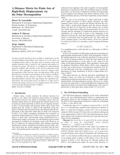
An open research question is how to define a useful metric on the
special Euclidean group SEn with respect to: (1) the choice of
coordinate frames and (2) the units used to measure linear and
angular distances that is useful for the synthesis and analysis of
mechanical systems. We discuss a technique for approximating
elements of SEn with elements of the special orthogonal group
SOn+1. This technique is based on using the singular value
decomposition (SVD) and the polar decompositions (PD) of the
homogeneous transform representation of the elements of SEn.
The embedding of the elements of SEn into SOn+1 yields
hyperdimensional rotations that approximate the rigid-body displacements.
The bi-invariant metric on SOn+1 is then used to
measure the distance between any two displacements. The result is
a left invariant PD based metric on SEn.
DOI: 10.1115/1.2735640
1 Introduction
Simply stated, a metric measures the distance between two
points in a set. There exist numerous useful metrics for defining
the distance between two points in Euclidean space; however,
defining similar metrics for determining the distance between two
locations of a finite rigid body is still an area of ongoing research.
In Ref. 1 Kazerounian and Rastegar define object norms that
depend upon the volume or shape of the rigid-body being displaced.
Geometrically motivated metrics that depend upon the displacement
of the rigid body rather than its shape were proposed
by Refs. 2,3. Gupta investigates Euclidean error measures on
rigid-body displacements 4. In Ref. 5 a Lie group theory approach
is taken and a left-invariant metric parameterized by a
characteristic length is presented. Lin and Burdick present formal
and practical conditions for kinematic metrics 6. Moreover, in
Ref. 7 addresses the inherent pitfalls when defining rigid-body
displacement metrics. Fanghella and Galletti present metric relations
based upon the closure equations associated with the kinematic
chain producing the motion 8. A local metric based on an
Contributed by the Mechanisms and Robotics Committee of ASME for publicationintheJOURNAL
OF MECHANICAL DESIGN. Manuscript received September 10,
2005; final manuscript received July 13, 2006. Review conducted by Kwun-Lon
Ting. Paper presented at the ASME 2005 Design Engineering Technical Conferences
and Computers and Information in Engineering Conference DETC2005, Long
Beach, CA, USA, September 24–28, 2005.
optimized local mapping of the study of quadric via stereographic
projection was proposed in Ref. 9. Chirikjian presents convolution
metrics on the group of rigid-body motions 10 and in Ref.
11 he compares and contrasts some metric methods. In Ref. 12
Belta and Kumar present a SVD based rigid-body motion interpolation.
In the cases of two locations of a finite rigid body in either
SE3 spatial locations or SE2 planar locations any Riemannian
metric used to measure the distance between the locations
yields a result which depends upon the chosen reference
frames see Refs. 5,7. However, for the specific case of orienting
a finite rigid body in SOn bi-invariant metrics do exist. For
example, Ravani and Roth 13 defined the distance between two
orientations of a rigid body in space as the magnitude of the
difference between the associated quaternions; a proof that this
metric is bi-invariant may be found in Ref. 2. One useful and
easily evaluated metric d on SOn follows. Given two elements
A1 and A2 of SOn we can define a metric using the Frobenius
norm as
d = I − A2A1T
F
1
It is straightforward to verify that this is a valid metric on SOn,
see Ref. 14.
In Ref. 2 Larochelle and McCarthy proposed an algorithm for
approximating displacements in SE2 with orientations in SO3.
By building upon the work of Ravani and Roth 13, they arrived
at a metric for planar locations in which the error induced by the
spherical approximation is on the order of 1/R 2 , where R is the
radius of the approximating sphere. Their algorithm is based upon
an algebraic formulation which utilizes Taylor series expansions
of sine and cosine terms in homogeneous transforms 15. Etzel
and McCarthy 16 later extended this work to spatial displacements
by using orientations in SO4 to approximate locations
in SE3.
This paper discusses an efficient alternative methodology for
defining a metric on a finite set of elements in SEn. Here, the
underlying geometrical motivations are the same—to approximate
displacements with hyperspherical rotations. However, we utilize
the polar decomposition to yield hyperspherical orientations that
approximate planar and spatial finite displacements. The work reported
here is built upon ideas found in Refs. 17,18,15,19.
2 The SVD-Based Embedding
The SVD-based approach, analogous to the works summarized
above, also uses hyperdimensional rotations to approximate displacements.
However, this technique uses products derived from
the SVD of the homogeneous transform to realize the embedding
of SEn−1 into SOn 20.
Consider the space of nn matrices as shown in Fig. 1. Let T
be a nn homogeneous transform that represents an element of
SEn−1. Note that T defines a point in Rn2. A is the desired
element of SOn nearest T when it lies in a direction orthogonal
to the tangent plane to SOn at A. The following theorem, based
upon related works by Hanson and Norris 21, provides the foundation
for the embedding,
Theorem 2.1. Given any nn matrix T, the closest element
of SO(n) is given by: A=UVT where T=U
diags1,s 2,...,snVT is the SVD of T.
Shoemake and Duff 19 prove that matrix A satisfies the
following optimization problem: Minimize: A−T 2
F subject to:
ATA−I=0, where A−T 2
F=i,ja
ij−t ij2 is used to denote
the Frobenius norm. Since A minimizes the Frobenius norm
in Rn2, it is the element of SOn that lies in a direction orthogonal
to the tangent plane of SOn at R. Hence, A is the closest
element of SOn to T. Moreover, for full-rank matrices the
SVD is well defined and unique. We now restate Theorem 2.1
Journal of Mechanical Design Copyright © 2007 by ASME
AUGUST 2007, Vol. 129 / 883
Downloaded 06 Aug 2007 to 163.118.202.33. Redistribution subject to ASME license or copyright, see http://www.asme.org/terms/Terms_Use.cfm

Fig. 1 The embedding of elements of SE„n−1… in SO„n…
with respect to the desired SVD based embedding of SEn−1
into SOn.
Theorem 2.2. For TSEn−1 and T=U
diags 1,s 2,...,s nV T , if A=UV T , then A is the unique
element of SOn nearest T.
Recall that T, the homogenous representation of SEn, isof
full rank 22 and, therefore, A exists, is well defined, and
unique.
3 The PD-Based Embedding
The polar decomposition PD though perhaps less known than
the SVD, is quite powerful and actually provides the foundation
for the SVD 23. Cauchy’s polar decomposition theorem states
that “a nonsingular matrix equals an orthogonal matrix either preor
post-multiplied by a positive definite symmetric matrix” 24.
With respect to our application, for T SEn−1 its PD is T
=PQ, where P and Q are nn matrices such that P is
orthogonal and Q is positive definite and symmetric. Recalling
the properties of the SVD, the decomposition of T yields U
diags1,s 2,...,sn−1VT , where matrices U and V are orthogonal
and matrix diags1,s 2,...,sn−1 is positive definite and
symmetric. Moreover, it is known that for full rank square matrices
the PD and the SVD are related by: P=UVT and Q
=Vdiags1,s 2,...,sn−1VT 23. Hence, for A=UVT we
have A P and conclude that the polar decomposition yields
the same element of SOn. We now restate Theorem 2.2 with
respect to the desired PD based embedding of SEn−1 onto
SOn.
Theorem 3.1. If TSEn−1 and P & Q, are the PD of
T such that T=PQ, then P is the unique element of SO(n)
nearest T.
Dubrulle 25 provides an algorithm for computing the PD that
produces monotonic convergence in the Frobenius norm that “...
generally delivers an IEEE double-precision solution in 10 or
fewer steps.”
4 Implementation of the Metric
The PD-based embedding of SEn−1 into SOn reviewed
above could be used for the systematic embedding of elements of
SEn−1 into SOn. However, to yield a useful metric for a finite
set of displacements appropriate for design, the principal axes
frame and the characteristic length are introduced.
4.1 The Principal Axes Frame. We now consider a finite set
of n displacements n2 and seek their magnitudes. In order to
yield a left-invariant metric, we build upon the work of Kazerounian
and Rastegar 1 in which approximately bi-invariant metrics
were defined for a prescribed finite rigid body. Here, to avoid
cumbersome volume integrals over the body we utilize a unit
point mass model for the moving body, the rationale being that the
moving frame in the application areas considered has some inherent
importance. For example, in robot end-effector applications
the moving frame will often be defined with its origin at the tool
center point. Moreover, in motion synthesis tasks, the moving
frame is often defined with its origin at the point on the moving
body whose motion is critical to the task at hand.
We proceed by determining the position vector of the center of
mass c and the principal axes frame PF associated with the n
prescribed locations, where a unit point mass is located at the
origin of each location
c = 1
n n
d
i=1
i
2
where d i is the translation vector associated with the ith location
i.e., the origin of the ith location with respect to the fixed frame.
Next, we define PF with its axes defined as the principal axes of
the inertia tensor I of the n point mass system about the centroid
c. First, we determine the inertia tensor I associated with the n
point mass system
n
I = 1 d
i=1
i 2 − d
i=1
id i T
3
where 1 is the 33 spatial or 22 planar identity matrix.
Finally, we determine the principal axes frame PF
PF = v 1 v 2 v 3 c
4
0 0 0 1
where v i are the unit eigenvectors of the inertia tensor I. The
directions of the vectors along the principal axes v i are chosen
such that PF is a right-handed system. The center of mass and the
principal axes frame are unique for the mechanical system and
invariant with respect to both the choice of coordinate frames and
the system of units 27,28. Note that the principal frame is not
dependent on the orientations of the frames at hand—only the
positions of their origins. However, the metric is dependent on the
orientations of the frames.
4.2 Characteristic Length. In order to resolve the unit disparity
between translations and rotations we use a characteristic
length to normalize the translational terms in the displacements.
There are three general approaches to selecting a characteristic
length: based upon the body being displaced 1,7, based upon the
kinematic chain generating the motion 8, or based upon the motion
task 29,5. The characteristic length we chose is R=24L/,
where L is the maximum translational component in the set of
displacements at hand. This formulation is based upon the motion
task and is reported in Refs. 2,16. This characteristic length is
the radius of the hypersphere that approximates the translational
terms by angular displacements that are 7.5 deg. It was shown
in Ref. 30 that this radius yields an effective balance. Note that
the metric presented here is not dependent upon this particular
choice of characteristic length and that, if so desired, an alternative
formulation may be utilized.
4.3 Step by Step. We now summarize the implementation of
the methodology. For a set of n locations, proceed as follows:
1. Determine PF associated with the n displacements;
2. Determine the relative displacements from PF to each of the
n locations;
884 / Vol. 129, AUGUST 2007 Transactions of the ASME
Downloaded 06 Aug 2007 to 163.118.202.33. Redistribution subject to ASME license or copyright, see http://www.asme.org/terms/Terms_Use.cfm
n

Table 1 Eleven planar locations
No. a b
deg
T
1 −1.0000 −1.0000 90.0000 0.1237
2 −1.2390 −0.5529 77.3621 0.3214
3 −1.4204 0.3232 55.0347 0.8455
4 −1.1668 1.2858 30.1974 1.4039
5 −0.5657 1.8871 10.0210 1.8118
6 −0.0292 1.9547 1.7120 1.9641
7 0.2632 1.5598 10.0300 1.8109
8 0.5679 0.9339 30.1974 1.4023
9 1.0621 0.3645 55.0346 0.8434
10 1.6311 0.0632 77.3620 0.3214
11 2.0000 0.0000 90.0000 0.1350
3. Determine the characteristic length R associated with the n
relative displacements and scale the translation terms in each
by 1/R;
4. Compute the elements of SO3planar or SO4spatial
associated with PF and each of the scaled relative displacements
using Theorem 3.1; and
5. The magnitude of the ith displacement is defined as the distance
from PF to the ith scaled relative displacement as computed
via Eq. 1. The distance between any two of the n
locations is similarly computed via the application of Eq. 1
to the scaled relative displacements embedded in SO3 or
SO4.
We note that since the center of mass and PF are invariant with
respect to both the choice of coordinate frames and the system of
units 27,28, that the polar decomposition displacement metric is
left invariant. The subsequent examples illustrate the application
of the above methodology to a finite set of planar or spatial displacements.
5 Example 1
Consider the 11 planar locations that define a motion generation
task proposed by J. Michael McCarthy of U.C. Irvine for the 2002
ASME Mechanisms & Robotics Conference and found in Ref.
26. The 11 a,b, locations are listed in Table 1 and shown in
Fig. 2 along with the fixed reference frame F where the x axes are
shown in reddark and the y axes in greenlight. We proceed as
above and determine PF
Fig. 2 The 11 planar locations and PF
Fig. 3 The fixed frame and four locations equidistant to location
No. 1
0.0067 − 1.0000 0.0094
PF = 1.0000 0.0067 0.6199
5 0 0 1
The 11 locations are now determined with respect to PF and the
maximum translational component is found to be 1.4278 and the
associated characteristic length is R=241.4278/=10.9073. Finally,
the magnitude of each of the displacements is computed via
Eq. 1 and listed in Table 1. To illustrate the applicabilility of the
metric to tasks such as motion, synthesis, motion, interpolation,
etc., we show four arbitrary locations that are equidistant to location
No. 1 in Fig. 3.
6 Example 2
Consider four spatial locations from the rigid-body motion generation
example presented in Ref. 31. The four locations are
listed in Table 2, and their associated PF is
0.5692
− 0.7807
PF =−
− 0.2578
0.8061
− 0.5916
0.0117
− 0.1617
− 0.2012
0.9661
0.75000
1.5000
0.4375
6
0 0 0 1
Next, the four locations with respect to the principal frame are
determined. The maximum translational component is found to be
1.7108 and the associated characteristic length is R=13.0695. Finally,
the magnitude of each of the displacements is listed in Table
2. Note that the magnitude of the first location is not zero because
the relative displacement from PF to the first location is nonidentity.
No. x y z
Table 2 Four spatial locations
deg
deg
deg
T
1 0.00 0.00 0.00 0.0 0.0 0.0 2.5281
2 0.00 1.00 0.25 15.0 15.0 0.0 2.5701
3 1.00 2.00 0.50 45.0 60.0 0.0 2.7953
4 2.00 3.00 1.00 45.0 80.0 0.0 2.8057
Journal of Mechanical Design AUGUST 2007, Vol. 129 / 885
Downloaded 06 Aug 2007 to 163.118.202.33. Redistribution subject to ASME license or copyright, see http://www.asme.org/terms/Terms_Use.cfm

7 Conclusions
We discussed a methodology for measuring distances on a finite
set of elements of SEn. This technique is based on embedding
SEn into SOn+1 via either the polar or the singular value
decompositions of the homogeneous transform representation of
SEn. A bi-invariant metric on SOn+1 is then used to measure
the distance between any two displacements SEn. The resulting
distance measure was shown to be left invariant. A detailed methodology
for applying this technique was presented and illustrated
by two examples.
ACKNOWLEDGMENT
This material is based upon work supported by the National
Science Foundation under Grants Nos. 0422705 and 0422731.
Any opinions, findings, and conclusions or recommendations expressed
in this material are those of the authors and do not
necessarily reflect the views of the National Science Foundation.
References
1 Kazerounian, K., and Rastegar, J., 1992. “Object Norms: A Class of Coordinate
and Metric Independent Norms for Displacements,” Proc. of the ASME
Design Engineering Technical Conferences, Scotsdale, AZ, September 13–16.
2 Larochelle, P., and McCarthy, J. M., 1995. “Planar Motion Synthesis Using an
Approximate Bi-invariant Metric,” ASME J. Mech. Des., 1174, pp. 646–
651.
3 Tse, D. M., and Larochelle, P. M., 2000. “Approximating Spatial Locations
with Spherical Orientations for Spherical Mechanism Design,” ASME J.
Mech. Des., 122, pp. 457–463.
4 Gupta, K. C., 1997. “Measures of Positional Error for a Rigid Body,” ASME
J. Mech. Des., 119, pp. 346–349.
5 Park, F. C., 1995. “Distance Metrics on the Rigid-body Motions with Applications
to Mechanism Design,” ASME J. Mech. Des., 1171, pp. 48–54.
6 Lin, Q., and Burdick, J., 2000. “Objective and Frame-Invariant Kinematic
Metric Functions for Rigid Bodies,” Int. J. Robot. Res., 196, pp. 612–625.
7 Martinez, J. M. R., and Duffy, J., 1995. “On the Metrics of Rigid Body Displacements
for Infinite and Finite Bodies,” ASME J. Mech. Des., 117, pp.
41–47.
8 Fanghela, P., and Galletti, C., 1995. “Metric Relations and Displacement
Groups in Mechansims and Robot Kinematics,” ASME J. Mech. Des., 1173,
pp. 470–478.
9 Eberharter, J., and Ravani, B., 2004. “Local Metrics for Rigid Body Displacements,”
ASME J. Mech. Des., 126, pp. 805–812.
10 Chirikjian, G. S., 1998. “Convolution Metrics for Rigid Body Motion,” Proc.
of the ASME Design Engineering Technical Conferences, Atlanta, CA, September
13–16.
11 Chirikjian, G. S., and Zhou, S., 1998. “Metrics on Motion and Deformation of
Solid Models,” ASME J. Mech. Des., 1202, pp. 252–261.
12 Belta, C., and Kumar, V., 2002. “An SVD-Based Projection Method for Interpolation
on SE3,” IEEE Trans. Rob. Autom., 183, pp. 334–345.
13 Ravani, B., and Roth, B., 1983. “Motion Synthesis using Kinematic Mappings,”
ASME J. Mech., Transm., Autom. Des., 105, pp. 460–467.
14 Schilling, R. J., and Lee, H., 1988. Engineering Analysis- a Vector Space
Approach, Wiley, New York.
15 McCarthy, J. M., 1983. “Planar and Spatial Rigid Body Motion as Special
Cases of Spherical and 3-Spherical Motion,” ASME J. Mech., Transm., Autom.
Des., 105, pp. 569–575.
16 Etzel, K., and McCarthy, J. M., 1996. “A Metric for Spatial Displacements
using Biquaternions on SO4,” Proc. of the IEEE International Conference on
Robotics and Automation, Minneapolis, MN, April 22–28.
17 Inonu, I., and Wigner, E., 1953. “On the Contraction of Groups and their
Representations,” Proc. Natl. Acad. Sci. U.S.A., 396, pp. 510–524.
18 Saletan, E., 1961. “Contraction of Lie Groups,” J. Math. Phys., 21, pp. 1–21.
19 Shoemake, K., and Duff, T., 1992. “Matrix Animation and Polar Decomposition,”
Proc. of Graphics Interface ’92, pp. 258–264, Vancouver, British Columbia,
Canada, May 11–15.
20 Larochelle, P., Murray, A., and Angeles, J., 2004. “SVD and PD Based Projection
Metrics on SEn,” Proc. On Advances in Robot Kinematics, Sestri
Levante, Italy, June 27–July 1.
21 Hanson, R. J., and Norris, M. J., 1981. “Analysis of Measurements Based upon
the Singular Value Decomposition,” SIAM Soc. Ind. Appl. Math. J. Sci. Stat.
Comput., 23, pp. 308–313.
22 Paul, R., 1981. Robot Manipulators: Mathematics, Programming, and Control,
MIT Press, Cambridge, MA.
23 Faddeeva, V. N., 1959. Computational Methods of Linear Algebra. Dover,
New York.
24 Halmos, P. R., 1990. Finite Dimensional Vector Spaces, Van Nostrand, Reinhold,
New York.
25 Dubrulle, A. A., 2001. “An Optimum Iteration for the Matrix Polar Decomposition,”
Electron. Trans. Numer. Anal., 8, pp. 21–25.
26 Al-Widyan, K., and Angeles, J., 2002. “A Numerically Robust Algorithm to
Solve the Five-Pose Burmester Problem,” Proc. of the ASME Design Engineering
Technical Conferences, Montréal, Canada, September 29–October 2.
27 Greenwood, D. T., 2003. Advanced Dynamics, Cambridge University Press,
Cambridge, UK.
28 Angeles, J., 2003. Fundamentals of Robotic Mechanical Systems, Springer,
New York.
29 Angeles, J., 2005. “Is there a Characteristic Length of a Rigid-body Displacement,”
Proc. of the 2005 International Workshop on Computational Kinematics,
Cassino, Italy, May 4–6.
30 Larochelle, P., 1999. “On the Geometry of Approximate Bi-invariant Projective
Displacement Metrics,” Proc. of the World Congress on the Theory of
Machines and Mechanisms, Oulu, Finland, June 20–24.
31 Larochelle, P., and Vance, J., 2000. “Interactive Visualization of the Line Congruences
Associated with Four Finite Spatial Positions,” Proceedings of the
Symposium Commemorating the Legacy, Works, and Life of Sir Robert Stawell
Ball upon the 100th Anniversary of the Publication of his Seminal Work A
Treatise on the Theory of Screws, University of Cambridge, Trinity College,
UK, July 9–11.
886 / Vol. 129, AUGUST 2007 Transactions of the ASME
Downloaded 06 Aug 2007 to 163.118.202.33. Redistribution subject to ASME license or copyright, see http://www.asme.org/terms/Terms_Use.cfm