A Displacement Metric for Finite Sets of Rigid Body Displacements

Proceedings of the ASME 2008 International Design Engineering Technical Conferences & Computers and
Information in Engineering Conference
Proceedings ofIDETC/CIE IDETC/CIE 2008
ASME 2008 International Design August Engineering 3-6, 2008, Brooklyn, TechnicalNew Conferences York, USA &
Computers and Information in Engineering Conference
August 3-6, 2008, New York, USA
DETC2008-49554
A DISPLACEMENT METRIC FOR FINITE SETS OF RIGID BODY DISPLACEMENTS
Venkatesh Venkataramanujam
Robotics & Spatial Systems Laboratory
Department of Mechanical and Aerospace Engineering
Florida Institute of Technology
Melbourne, Florida 32901
Email: vvenkata@fit.edu
ABSTRACT
There are various useful metrics for finding the distance
between two points in Euclidean space. Metrics for finding
the distance between two rigid body locations 1 in Euclidean
space depend on both the coordinate frame and units used. A
metric independent of these choices is desirable. This paper
presents a metric for a finite set of rigid body displacements.
The methodology uses the principal frame (PF) associated with
the finite set of displacements and the polar decomposition to
map the homogenous transform representation of elements of the
special Euclidean group SE(N-1) onto the special orthogonal
group SO(N). Once the elements are mapped to SO(N) a biinvariant
metric can then be used. The metric obtained is thus
independent of the choice of fixed coordinate frame i.e. it is
left invariant. This metric has potential applications in motion
synthesis, motion generation and interpolation. Three examples
are presented to illustrate the usefulness of this methodology.
INTRODUCTION
A metric is used to measure the distance between two points
in a set. There are various metrics for finding the distance
between two points in Euclidean space. However, finding the
distance between two locations of a rigid body is still the
subject of ongoing research, see [1–9]. For two locations of
a finite rigid body (either SE(2)-planar or SE(3)-spatial) all
∗ Address all correspondence to this author.
1 Location of a rigid body prescribes both its position and orientation.
Pierre Larochelle ∗
Robotics & Spatial Systems Laboratory
Department of Mechanical and Aerospace Engineering
Florida Institute of Technology
Melbourne, Florida 32901
Email: pierrel@fit.edu
SO(N)
R N2
[P]
[T]
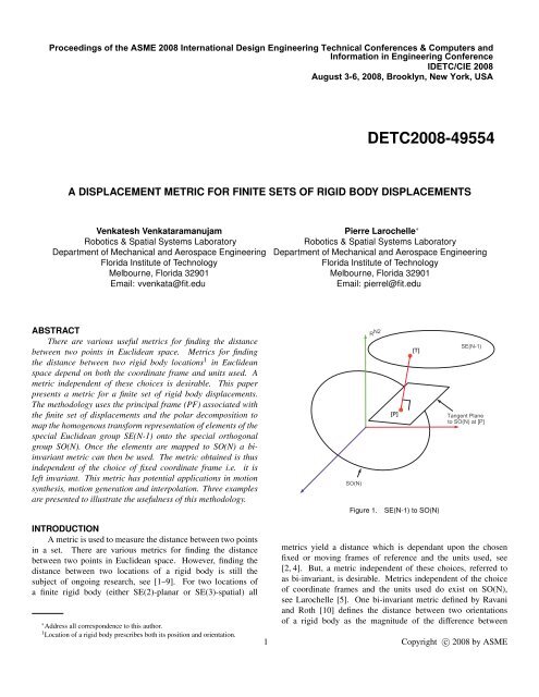
Figure 1. SE(N-1) to SO(N)
SE(N-1)
Tangent Plane
to SO(N) at [P]
metrics yield a distance which is dependant upon the chosen
fixed or moving frames of reference and the units used, see
[2, 4]. But, a metric independent of these choices, referred to
as bi-invariant, is desirable. Metrics independent of the choice
of coordinate frames and the units used do exist on SO(N),
see Larochelle [5]. One bi-invariant metric defined by Ravani
and Roth [10] defines the distance between two orientations
of a rigid body as the magnitude of the difference between
1 Copyright c○ 2008 by ASME

F
x
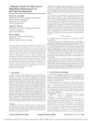
the associated quaternions. The techniques presented here are
based on the polar decomposition (PD) of the homogenous
transform representation of the elements of SE(N) and the
principal frame (PF) associated with the finite set of rigid body
displacements. The mapping of the elements of the special
Euclidean group SE(N-1) to SO(N) yields hyperdimensional
rotations that approximate the rigid body displacements. A
conceptual representation of the mapping of SE(N-1) to SO(N)
is shown in Figure 1. Once the elements are mapped to SO(N)
distances can then be evaluated by using a bi-invariant metric
on SO(N). In the planar case the elements of SE(2) are mapped
onto the SO(3) as shown in Figure 2. The resulting PD based
projection metric on SE(N-1) is left invariant (i.e. independent
of the choice of fixed frame F).
METRIC ON SO(N)
The distance between elements in SO(N) can be determined
by using the metric suggested by Larochelle [11]. The distance
between two elements [A1] and [A2] in SO(N) can be defined by
using the Frobenius norm as follows,
d = [I] − [A2][A1] T F
FINITE SETS OF LOCATIONS
Consider the case when a finite number of n displacements
(n≥2) are given and we have to find the magnitude of these
displacements. The displacements depend on the coordinate
frame and the system of units chosen. In order to yield a left
invariant metric we utilize a PF that is derived from a unit point
y
ψ
M
Figure 2. SE(2) to SO(3)
(1)
2
1.5
1
0.5
0
−0.5
−1
F
θ
M3
M
φ
M4
M2
M1
ψ
M5
M6
F
PF
M7
−1.5 −1 −0.5 0 0.5 1 1.5 2
M8
M9
Figure 3. Unit Point Mass Model
mass model for a moving body as suggested by Larochelle [11].
This is done to yield a metric that is independent of the geometry
of the moving body. The center of mass and the principal axes
frame are unique for the system and invariant with respect to
both the choice of fixed coordinate frames as well as the system
of units [12, 13].
The procedure for determining the center of mass −→ c and
the PF associated with the n prescribed locations is described
2 Copyright c○ 2008 by ASME
M10
M11

elow. A unit point mass is located at the origin of each location
as shown in Figure 3.
−→ 1
c =
n
where, −→ di is the translation vector associated with the i th location
(i.e. the origin of the i th location with respect to F).
The PF is defined such that its axes are aligned with the
principal axes of the n point mass system and its origin is at
the centroid −→ c . After finding the centroid of the system we
determine the principal axes of the point mass system. The
inertia tensor is,
[I] =
⎡
n
∑
i=1
−→ di
⎣ Ixx Ixy Ixz
Iyx Iyy Iyz
Izx Izy Izz
⎤
(2)
⎦ (3)
where the principal moments of inertia are defined by,
the products of inertia are,
n
Ixx = ∑
i=1
n
Iyy = ∑
i=1
n
Izz = ∑
i=1
Ixy = Iyx = −
Ixz = Izx = −
Iyz = Izy = −
(y 2 i + z 2 i )
(z 2 i + x 2 i ) (4)
(x 2 i + y 2 i )
n
∑
i=1
n
∑
i=1
n
∑
i=1
(xiyi)
(xizi) (5)
(yizi)
and xi, yi, zi are the components of −→ di . The principal frame is
thus determined to be
−→v1
[PF] =
−→ v2 −→ v3 −→
c
0 0 0 1
where, −→ vi are the principal axes (eigenvectors) associated with
the inertia tensor [I], see Greenwood [12]. The directions of
the vectors along the principal axes −→ vi are chosen such that the
(6)
principal frame is a right handed system. However, Equation (6)
does not uniquely define the PF since the eigenvectors −→ vi of the
inertia tensor are not unique; both −→ vi and − −→ vi are eigenvectors
associated with [I]. In order to resolve this ambiguity and yield a
unique PF we choose to use the PF that is most closely aligned
to F.
In the planar case the inertia tensor [I] reduces to
⎡
[I] = ⎣ Ixx
Iyx
Ixy
Iyy
⎤
0
0 ⎦ (7)
0 0 1
and, the principal frame for the planar case reduces to a 3 × 3
matrix as shown:
−→v1
[PF] =
−→ v2 −→
c
0 0 1
The eight different right handed PF’s that are possible in the
spatial case are given by,
[ −→ v1 −→ v2 −→ v3 ]
[ −→ v2 - −→ v1 −→ v3 ]
[- −→ v1 - −→ v2 −→ v3 ]
[- −→ v2 −→ v1 −→ v3 ]
[ −→ v2 −→ v1 - −→ v3 ]
[ −→ v1 - −→ v2 - −→ v3 ]
[- −→ v2 - −→ v1 - −→ v3 ]
[- −→ v1 −→ v2 - −→ v3 ]
In the planar case there are four possible orientations of the PF
as seen in Figure 4.
[ −→ v1 −→ v2 ]
[ −→ v2 - −→ v1 ]
[ −→ v1 - −→ v2 ]
[- −→ v2 −→ v1 ]
The PF that is most closely oriented to the fixed frame is chosen
using the metric on SO(N) given in Equation (1).
MAPPING TO SO(N)
The unit disparity between translation and rotation is resolved
by normalizing the translational terms in displacements.
The displacements are normalized by choosing a characteristic
length R. The characteristic length used, based upon the investigations
reported in [5, 14], is 24L
π , where L is the maximum
translational component in the set of displacements at hand.
Larger characteristic lengths result in an increase in the weight
on the rotational terms whereas smaller ones result in an increase
in weight on the translational terms. It was shown in [14] that
3 Copyright c○ 2008 by ASME
(8)

Fixed Frame
v 2
Figure 4. Four Possible Orientations for the PF
this characteristic length yields an effective balance between
translational and rotational displacement terms for projection
metrics.
The elements in SO(N) are derived from the polar decomposition
of the homogenous transformations representing planar
SE(2) or spatial SE(3) displacements. A number of iterative
algorithms exist for the evaluation of the polar decomposition.
Hingham described a method based upon Newtons method,
see [15]. A simple and efficient iterative algorithm for the
computation of the polar decomposition is shown by Dubrulle
[16]. The algorithm produces mono-tonic convergence in the
Frobenius norm that delivers an IEEE solution [17] in ∼ 10 or
fewer steps.
The elements SE(N) in the planar and spatial cases are
represented by,
and,
Ti =
Ti =
⎡
⎤
⎢
⎣
[R] −→ t ⎥
⎦
0 0 1
⎡
⎤
⎢
⎣
[R] −→ t ⎥
⎦
0 0 0 1
v 1
(9)
(10)
where [R] represents the rotational component and −→ t represents
the translational component of the homogenous transformation
of the locations. The scaled transformation matrices for the
planar and spatial cases are thus obtained to be,
and
⎡
⎤
⎢
Ti(scaled) = ⎢
⎣
[R] −→ t /R ⎥
⎦
0 0 1
⎡
⎤
⎢
Ti(scaled) = ⎢
⎣
[R] −→ t /R ⎥
⎦
0 0 0 1
(11)
(12)
where, R represents the characteristic length used to resolve
the unit disparity between rotation and translation. The scaled
transformation matrices may then be mapped to SO(N) by using
the Dubrulle algorithm for PD.
SUMMARY OF THE TECHNIQUE
For a set of n finite rigid body locations the steps to be
followed are:
1. Determine the PF associated with the n locations.
2. Determine the relative displacements from PF to each of the
n locations.
3. Determine the characteristic length R associated with the n
displacements with respect to the PF and scale the translation
terms in each by 1/R.
4. Compute the projections of PF and each of the scaled relative
displacements using the polar decomposition algorithm.
5. The magnitude of the displacement is defined as the distance
from PF to the scaled relative displacement as computed
via Equation (1). The distance between any two of the
n locations is similarly computed by the application of
Equation (1) to the projected scaled relative displacements.
EXAMPLE: ELEVEN PLANAR LOCATIONS
Consider the rigid body guidance problem proposed by J.
Michael McCarthy, U.C. Irvine for the 2002 ASME International
Design Engineering Technical Conferences held in Montreal,
Quebec and listed in [18]. The 11 planar locations are listed
in Table 1 and the origins of the coordinate frames with the
respect to the fixed reference frame F are shown in Figure 3. The
centroid of the system is determined to be −→ c = [0.0094 0.6199] T .
Next, the principal axes directions are determined. The principal
4 Copyright c○ 2008 by ASME

2
1.5
1
0.5
0
−0.5
−1
M3
M4
M2
M1
M5
M6
PF
F
M7
−1.5 −1 −0.5 0 0.5 1 1.5 2
Figure 5. Principal Frame for Eleven Desired Locations
axes directions and −→ c are used to determine the principal frame.
M8
⎡
⎤
1.0000 0.0067 0.0094
[PF] = ⎣ -0.0067 1.0000 0.6199 ⎦ (13)
0.0000 0.0000 1.0000
The eleven locations are now determined with respect to the PF
and the maximum translational component is found to be 1.9947
and the resulting characteristic length R = 24L
π = 15.239. The 11
locations are then scaled by the characteristic length in order to
find the distance to the principal frame. The magnitude of each
of the displacements with respect to the PF is listed in Table 1.
The distance between any two of the locations is computed by
the application of Equation (1) to the projected scaled relative
displacements. For example the distance between location #1
and location #2 was found to be 0.3115.
EXAMPLE: FOUR SPATIAL LOCATIONS
Consider the rigid body guidance problem investigated by
Larochelle [11]. The 4 spatial locations are listed in Table 2 with
respect to the fixed reference frame F and are shown in Figure 6.
The principal frame is determined to be
⎡
⎤
0.8061 0.5692 -0.1617 0.7500
⎢
[PF] = ⎢ -0.5916 0.7807 -0.2012 1.5000 ⎥
⎣ 0.0117 0.2578 0.9661 0.4375 ⎦
0.0000 0.0000 0.0000 1.0000
M9
M10
M11
(14)
Table 1. Eleven Planar Locations
# x y α (deg) Mag.
1 −1.0000 −1.0000 90.0000 2.0076
2 −1.2390 −0.5529 77.3621 1.7762
3 −1.4204 0.3232 55.0347 1.3165
4 −1.1668 1.2858 30.1974 0.7483
5 −0.5657 1.8871 10.0210 0.2644
6 −0.0292 1.9547 1.7120 0.0807
7 0.2632 1.5598 10.0300 0.2606
8 0.5679 0.9339 30.1974 0.7464
9 1.0621 0.3645 55.0346 1.3159
10 1.6311 0.0632 77.3620 1.7762
11 2.0000 0.0000 90.0000 2.0078
Table 2. Four Desired Locations
# x y z θ φ ψ Mag.
1 0.00 0.00 0.00 0.0 0.0 0.0 0.95
2 0.00 1.00 0.25 15.0 15.0 0.0 1.24
3 1.00 2.00 0.50 45.0 60.0 0.0 2.21
4 2.00 3.00 1.00 45.0 80.0 0.0 2.44
The maximum translational component is found to be 2.0276
and the associated characteristic length is R = 15.4899. The
magnitude of each of the displacements with respect to the PF is
listed in Table 2.
EXAMPLE: TEN SPATIAL LOCATIONS
Consider the rigid body guidance problem investigated by
Larochelle [11]. The 10 spatial locations with respect to the
the fixed reference frame F are listed in Table 3 and shown in
Figure 7. The principal frame is given by,
⎡
⎤
0.756 0.655 0.000 5.500
⎢
[PF] = ⎢ 0.000 0.000 1.000 0.000 ⎥
⎣ 0.655 -0.756 0.000 0.000 ⎦
0.000 0.000 0.000 1.000
(15)
The maximum translational component L is found to be 6.7256
and the associated characteristic length is R = 24L
π = 51.3795.
5 Copyright c○ 2008 by ASME

F
T1
T2
PF
Figure 6. Principal Frame for Four Desired Locations
T1
F
T2
T3
T4
T5
Figure 7. Principal Frame for Ten Desired Locations
The distance from the first location to the principal frame was
found to be 2.7488. The distance between location #1 and
location #2 was found to be 0.3485.
CONCLUSIONS
We have developed a metric for a finite set of rigid body
displacements which uses a mapping of the special Euclidean
group SE(N-1). This technique is based on embedding SE(N-
1) into SO(N) via the polar decomposition of the homogeneous
transform representation of SE(N-1). To yield a useful metric for
a finite set of displacements appropriate for design applications,
the principal frame and the characteristic length are used. A bi-
T3
T6
PF
T7
T8
T9
T4
T10
Table 3. Ten Desired Locations.
# x y z Long (θ) Lat (φ) Roll (ψ)
1 1.00 0.00 5.00 100 0.00 0.00
2 2.00 0.00 4.00 90 0.00 10.00
3 3.00 0.00 3.00 80 0.00 20.00
4 4.00 0.00 2.00 70 0.00 30.00
5 5.00 0.00 1.00 60 0.00 40.00
6 6.00 0.00 −1.00 50 0.00 50.00
7 7.00 0.00 −2.00 40 0.00 60.00
8 8.00 0.00 −3.00 30 0.00 70.00
9 9.00 0.00 −4.00 20 0.00 80.00
10 10.00 0.00 −5.00 10 0.00 90.00
invariant metric on SO(N) is then used to measure the distance
between any two displacements in SE(N-1). A detailed algorithm
for the application of this method was presented and illustrated
by three examples. This technique has potential applications in
mechanism synthesis and robot motion planning.
ACKNOWLEDGMENT
This material is based upon work supported by the National
Science Foundation under grant #0422705. Any opinions,
findings, and conclusions or recommendations expressed in this
material are those of the authors and do not necessarily reflect
the views of the National Science Foundation.
REFERENCES
[1] Lin, Q., and Burdick, J., 2000. “Objective and frameinvariant
kinematic metric functions for rigid bodies”. International
Journal for Robotics Research, 19(6), pp. 612–
625.
[2] Park, F., 1995. “Distance metrics on the rigid-body motions
with applications to mechanism design”. ASME Journal of
Mechanical Design, 117(1), September, pp. 48–54.
[3] Kazerounian, K., and Rastegar, J., 1992. “Object norms:
A class of coordinate and metric independent norms for
displacements”. In Proceedings of the ASME 1998 Design
Engineering Technical Conferences and Computers and
Information Conference.
[4] Martinez, J. M. R., and Duffy, J., 1995. “On the metrics
of rigid body displacements for infinite and finite bodies”.
ASME Journal of Mechanical Design, 117(1), pp. 41–47.
[5] Larochelle, P., and McCarthy, J., 1995. “Planar motion
6 Copyright c○ 2008 by ASME

synthesis using an approximate bi-invariant metric”.
ASME Journal of Mechanical Design, 117(1), September,
pp. 646–651.
[6] Etzel, K., and McCarthy, J., 1996. “A metric for
spatial displacement using biquaternions on SO(4)”. In
Proceedings., 1996 IEEE International Conference on
Robotics and Automation.
[7] Gupta, K. C., 1997. “Measures of positional error for a
rigid body”. ASME Journal of Mechanical Design, 119(3),
pp. 346–348.
[8] Tse, D., and Larochelle, P., 2000. “Approximating
spatial locations with spherical orientations for spherical
mechanism design”. ASME Journal of Mechanical Design,
122(4), pp. 457–463.
[9] Eberharter, J., and Ravani, B., 2004. “Local metrics for
rigid body displacements”. ASME Journal of Mechanical
Design, 126, pp. 805–812.
[10] Ravani, B., and Roth, B., 1983. “Motion synthesis using
kinematic mappings”. ASME Journal of Mechanisms,
Transmissions, and Automation in Design, 105, pp. 460–
467.
[11] Larochelle, P., 2006. “A polar decomposition based
displacement metric for a finite region of SE(n)”. In
Proceedings of the 10th International Symposium on
Advances in Robot Kinematics (ARK), Lubljana, Slovenia.
[12] Greenwood, D., 2003. Advanced Dynamics. Cambridge
University Press.
[13] Angeles, J., 2003. Fundamentals of Robotic Mechanical
Systems. Springer.
[14] Larochelle, P., 1999. “On the geometry of approximate
bi-invariant projective displacement metrics”. Proceedings
of the World Congress on the Theory of Machines and
Mechanisms.
[15] J.Higham, N., 1986. “Computing the polar decomposition–
with applications”. SIAM Journal on Scientific and
Statistical Computing, 7(4), pp. 1160–1174.
[16] Dubrulle, A. A., 2001. “An optimum iteration for the
matrix polar decomposition”. In Electronic Transaction on
Numerical Analysis, Vol. 8, pp. 21–25.
[17] ANSI/IEEE, 1985. “IEEE standard for binary floatingpoint
arithmetic”. ANSI/IEEE Standard 754-1985.
[18] Al-Widyan, K., Cervantes-Sànchez, J. J., and Angeles, J.,
2002. “A numericaly robust algorithm to solve the five-pose
burmester problem”. In Proceedings of the ASME Design
Engineering Technical Conferences, ASME International.
7 Copyright c○ 2008 by ASME