A Displacement Metric for Finite Sets of Rigid Body Displacements

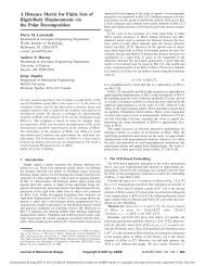
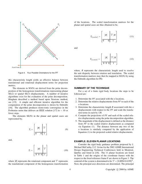
Fixed Frame
v 2
Figure 4. Four Possible Orientations for the PF
this characteristic length yields an effective balance between
translational and rotational displacement terms for projection
metrics.
The elements in SO(N) are derived from the polar decomposition
of the homogenous transformations representing planar
SE(2) or spatial SE(3) displacements. A number of iterative
algorithms exist for the evaluation of the polar decomposition.
Hingham described a method based upon Newtons method,
see [15]. A simple and efficient iterative algorithm for the
computation of the polar decomposition is shown by Dubrulle
[16]. The algorithm produces mono-tonic convergence in the
Frobenius norm that delivers an IEEE solution [17] in ∼ 10 or
fewer steps.
The elements SE(N) in the planar and spatial cases are
represented by,
and,
Ti =
Ti =
⎡
⎤
⎢
⎣
[R] −→ t ⎥
⎦
0 0 1
⎡
⎤
⎢
⎣
[R] −→ t ⎥
⎦
0 0 0 1
v 1
(9)
(10)
where [R] represents the rotational component and −→ t represents
the translational component of the homogenous transformation
of the locations. The scaled transformation matrices for the
planar and spatial cases are thus obtained to be,
and
⎡
⎤
⎢
Ti(scaled) = ⎢
⎣
[R] −→ t /R ⎥
⎦
0 0 1
⎡
⎤
⎢
Ti(scaled) = ⎢
⎣
[R] −→ t /R ⎥
⎦
0 0 0 1
(11)
(12)
where, R represents the characteristic length used to resolve
the unit disparity between rotation and translation. The scaled
transformation matrices may then be mapped to SO(N) by using
the Dubrulle algorithm for PD.
SUMMARY OF THE TECHNIQUE
For a set of n finite rigid body locations the steps to be
followed are:
1. Determine the PF associated with the n locations.
2. Determine the relative displacements from PF to each of the
n locations.
3. Determine the characteristic length R associated with the n
displacements with respect to the PF and scale the translation
terms in each by 1/R.
4. Compute the projections of PF and each of the scaled relative
displacements using the polar decomposition algorithm.
5. The magnitude of the displacement is defined as the distance
from PF to the scaled relative displacement as computed
via Equation (1). The distance between any two of the
n locations is similarly computed by the application of
Equation (1) to the projected scaled relative displacements.
EXAMPLE: ELEVEN PLANAR LOCATIONS
Consider the rigid body guidance problem proposed by J.
Michael McCarthy, U.C. Irvine for the 2002 ASME International
Design Engineering Technical Conferences held in Montreal,
Quebec and listed in [18]. The 11 planar locations are listed
in Table 1 and the origins of the coordinate frames with the
respect to the fixed reference frame F are shown in Figure 3. The
centroid of the system is determined to be −→ c = [0.0094 0.6199] T .
Next, the principal axes directions are determined. The principal
4 Copyright c○ 2008 by ASME