A Displacement Metric for Finite Sets of Rigid Body Displacements

More documents

Recommendations

Info

F x the associated quaternions. The techniques presented here are based on the polar decomposition (PD) of the homogenous transform representation of the elements of SE(N) and the principal frame (PF) associated with the finite set of rigid body displacements. The mapping of the elements of the special Euclidean group SE(N-1) to SO(N) yields hyperdimensional rotations that approximate the rigid body displacements. A conceptual representation of the mapping of SE(N-1) to SO(N) is shown in Figure 1. 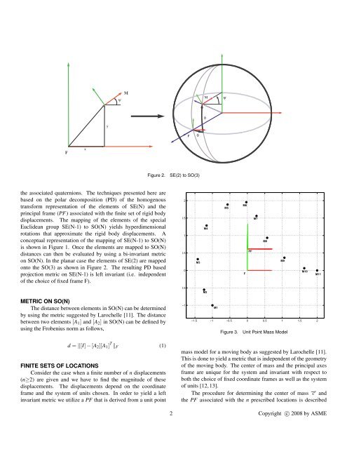Once the elements are mapped to SO(N) distances can then be evaluated by using a bi-invariant metric on SO(N). In the planar case the elements of SE(2) are mapped onto the SO(3) as shown in Figure 2. The resulting PD based projection metric on SE(N-1) is left invariant (i.e. independent of the choice of fixed frame F). METRIC ON SO(N) The distance between elements in SO(N) can be determined by using the metric suggested by Larochelle [11]. The distance between two elements [A1] and [A2] in SO(N) can be defined by using the Frobenius norm as follows, d = [I] − [A2][A1] T F FINITE SETS OF LOCATIONS Consider the case when a finite number of n displacements (n≥2) are given and we have to find the magnitude of these displacements. The displacements depend on the coordinate frame and the system of units chosen. In order to yield a left invariant metric we utilize a PF that is derived from a unit point y ψ M Figure 2. SE(2) to SO(3) (1) 2 1.5 1 0.5 0 −0.5 −1 F θ M3 M φ M4 M2 M1 ψ M5 M6 F PF M7 −1.5 −1 −0.5 0 0.5 1 1.5 2 M8 M9 Figure 3. Unit Point Mass Model mass model for a moving body as suggested by Larochelle [11]. This is done to yield a metric that is independent of the geometry of the moving body. The center of mass and the principal axes frame are unique for the system and invariant with respect to both the choice of fixed coordinate frames as well as the system of units [12, 13]. The procedure for determining the center of mass −→ c and the PF associated with the n prescribed locations is described 2 Copyright c○ 2008 by ASME M10 M11
elow. A unit point mass is located at the origin of each location as shown in Figure 3. −→ 1 c = n where, −→ di is the translation vector associated with the i th location (i.e. the origin of the i th location with respect to F). The PF is defined such that its axes are aligned with the principal axes of the n point mass system and its origin is at the centroid −→ c . After finding the centroid of the system we determine the principal axes of the point mass system. The inertia tensor is, [I] = ⎡ n ∑ i=1 −→ di ⎣ Ixx Ixy Ixz Iyx Iyy Iyz Izx Izy Izz ⎤ (2) ⎦ (3) where the principal moments of inertia are defined by, the products of inertia are, n Ixx = ∑ i=1 n Iyy = ∑ i=1 n Izz = ∑ i=1 Ixy = Iyx = − Ixz = Izx = − Iyz = Izy = − (y 2 i + z 2 i ) (z 2 i + x 2 i ) (4) (x 2 i + y 2 i ) n ∑ i=1 n ∑ i=1 n ∑ i=1 (xiyi) (xizi) (5) (yizi) and xi, yi, zi are the components of −→ di . The principal frame is thus determined to be −→v1 [PF] = −→ v2 −→ v3 −→ c 0 0 0 1 where, −→ vi are the principal axes (eigenvectors) associated with the inertia tensor [I], see Greenwood [12]. The directions of the vectors along the principal axes −→ vi are chosen such that the (6) principal frame is a right handed system. However, Equation (6) does not uniquely define the PF since the eigenvectors −→ vi of the inertia tensor are not unique; both −→ vi and − −→ vi are eigenvectors associated with [I]. In order to resolve this ambiguity and yield a unique PF we choose to use the PF that is most closely aligned to F. In the planar case the inertia tensor [I] reduces to ⎡ [I] = ⎣ Ixx Iyx Ixy Iyy ⎤ 0 0 ⎦ (7) 0 0 1 and, the principal frame for the planar case reduces to a 3 × 3 matrix as shown: −→v1 [PF] = −→ v2 −→ c 0 0 1 The eight different right handed PF’s that are possible in the spatial case are given by, [ −→ v1 −→ v2 −→ v3 ] [ −→ v2 - −→ v1 −→ v3 ] [- −→ v1 - −→ v2 −→ v3 ] [- −→ v2 −→ v1 −→ v3 ] [ −→ v2 −→ v1 - −→ v3 ] [ −→ v1 - −→ v2 - −→ v3 ] [- −→ v2 - −→ v1 - −→ v3 ] [- −→ v1 −→ v2 - −→ v3 ] In the planar case there are four possible orientations of the PF as seen in Figure 4. [ −→ v1 −→ v2 ] [ −→ v2 - −→ v1 ] [ −→ v1 - −→ v2 ] [- −→ v2 −→ v1 ] The PF that is most closely oriented to the fixed frame is chosen using the metric on SO(N) given in Equation (1). MAPPING TO SO(N) The unit disparity between translation and rotation is resolved by normalizing the translational terms in displacements. The displacements are normalized by choosing a characteristic length R. The characteristic length used, based upon the investigations reported in [5, 14], is 24L π , where L is the maximum translational component in the set of displacements at hand. Larger characteristic lengths result in an increase in the weight on the rotational terms whereas smaller ones result in an increase in weight on the translational terms. It was shown in [14] that 3 Copyright c○ 2008 by ASME (8)
Page 1: Proceedings of the ASME 2008 Intern
Page 5 and 6: 2 1.5 1 0.5 0 −0.5 −1 M3 M4 M2
Page 7: synthesis using an approximate bi-i

A Displacement Metric for Finite Sets of Rigid Body Displacements

You also want an ePaper? Increase the reach of your titles

Delete template?

Save as template?