sounding rocket trajectory simulation and optimization with astos - ESA

SOUNDING ROCKET TRAJECTORY SIMULATION AND OPTIMIZATION WITH
ASTOS
Francesco Cremaschi (1) , Sven Weikert (2) , Andreas Wiegand (3) , Wolfgang Jung (4) , Frank Scheuerpflug (5)
ABSTRACT
(1) Astos Solutions GmbH, Germany, Tel: +49-711-6723561-14, Email: francesco.cremaschi@astos.de
(2) Astos Solutions GmbH, Germany, Tel: +49-711-6723561-12, Email: sven.weikert@astos.de
(3) Astos Solutions GmbH, Germany, Tel: +49-7721-50142, Email: andreas.wiegand@astos.de
(4) DLR, Germany, Tel.: +49-8153-28-2724/2606, Email: wolfgang.jung@dlr.de
(5) DLR, Germany, Tel.: +49-8153-28-2724/2606, Email: frank.scheuerpflug@dlr.de
With a long experience in the simulation and
optimization of atmospheric trajectories (launcher and
re-entry vehicles), ASTOS [1], the AeroSpace
Trajectory Optimization Software, has been applied to
the sounding rocket environment. An extensive library
[2] of differential equations (3-DOF and 6-DOF),
vehicle models (propulsion, aerodynamics, etc.),
constraints and cost functions is available to the user, in
a friendly graphical user interface (GUI).
As a demonstration test-case, the simulation of the
SHEFEX II (SHarp Edge Flight EXperiment) mission is
presented. In collaboration with DLR MORABA
(Mobile Rocket Base), the available aerodynamics and
propulsion data has been inserted in ASTOS to
reproduce (through simulation) and improve (through
optimization) the trajectory. Furthermore the paper
depicts the post-processing features of the software: the
results can be displayed both numerically and
graphically, the first for a precise evaluation of the
trajectory data and the latter to provide a straightforward
overview of the mission. Safety aspects are covered by a
dispersion analysis of the impact position that completes
the paper.
1. ASTOS SOFTWARE TOOL
ASTOS is a simulation and optimization environment to
simulate and optimize trajectories for a variety of
complex, multi-phase optimal control problems. In the
last twenty years it has been successfully applied in
several industrial or ESA projects in the field of
launcher, re-entry and exploration missions. Just to
provide some examples: Ariane5, Vega, ATV, Hopper,
Skylon, Fly-back Booster, X38, Capree, ATPE, USV,
Smart-Olev, LEO, Astex, IXV, ARD, Expert, et. al.
ASTOS consists of fast and powerful optimization
programs, PROMIS, CAMTOS, SOCS and TROPIC,
that handle large and highly discretised problems, a user
interface with multiple-plot capability and an integrated
graphical iteration monitor to review the optimization
process and plot the state and control histories at
intermediate steps during the optimization.
ASTOS comprises an extensive model library, which
allows launcher and re-entry trajectory optimization
without programming work.
Figure 1. ASTOS multi screenshot
1.1. Batch Mode capability
___________________________________________________________________________________
Proc. ‘19th ESA Symposium on European Rocket and Balloon Programmes and Related Research,
Bad Reichenhall, Germany, 7–11 June 2009 (ESA SP-671, September 2009)
The “Batch Mode Inspector” (since ASTOS version 6.0)
enables the user to perform Monte Carlo analyses
without third-party tools and to plot the results directly
by means of ASTOS plotting capabilities. The user can
associate a batch variable to each model uncertainty.
Then, in the Batch Mode Inspector, he can build the
structure of the processes with which the batch variables
are used in order to run the model automatically over a
given parameter space. The structure consists of various
batch elements freely chosen by the user. These can be
actions like Initialize, Simulate, Optimize or postprocessing
elements that prepare the data taken from the
simulation for further analysis.
The batch variables may be modified by Loop and
Random elements. Loop will change a batch variable
monotonously from an initial value to a final one using
a given increment. Instead, with the Random element it
is possible to compute random numbers with Gaussian
or uniform distribution. Uniform distribution variables
are defined by a lower and upper bound, Gaussian by

their mean value and the standard deviation. Further
details are described in [1].
2. SHEFEX
Figure 2. Batch mode inspector
The Sharp Edge Flight Experiment is a DLR (German
Aerospace Centre) program to investigate aerodynamic
behaviour and thermal protection problems and develop
solutions for re-entry vehicles at hypersonic velocities,
using unconventional shapes comprising multi-facetted
surfaces with sharp edges. Sounding rockets provide a
useful facility to obtain experimental flight data for
period of several orders greater than possible with shock
tunnels. The first SHEFEX sounding rocket launch,
comprising an experiment with an asymmetric form at
re-entry velocities of Mach 6-7, was launched from the
Andoya Rocket Range (ARR), Norway, in October
2005. The success of this mission led to the definition
and approval of the SHEFEX 2 mission.
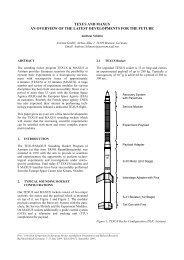
Figure 3. Artistic impression of SHEFEX2
SHEFEX 2 was originally conceived as a payload with
small passive stabilizing fins, to be flown on a VSB-30
with a conventional parabolic trajectory which would
have provided velocities in the order of Mach 8. The
greater velocity, together with a re-entry elevation angle
in the order of 75 degrees, would have resulted in a
short experiment time. An alternative solution was then
found in the VS-40 motor combination together with a
precession control of the spinning second stage to
provide a conventional trajectory of the first stage
together with a suppressed trajectory of the exoatmospheric
burning second stage. The result is a flatter
re-entry angle of about 35 degrees and a velocity of
Mach 10, which still provides in the order of 60 seconds
of experiment time between 100 and 20 kilometres
altitude.
The results are a vehicle and a payload that are the most
complex and challenging projects MORABA has
constructed and launched to date.
3. TRAJECTORY SIMULATION
As described in section 2, the SHEFEX 2 mission will
be launched by a two stage sounding rocket. The
workflow to simulate a trajectory in ASTOS is intuitive
and in line with the logic of the mission design
engineer. The first steps are performed in the Model
Browser, the GUI that links all the models of the
ASTOS library.
3.1. Modelling the Vehicle
- Define the environment either from a list of already
available models or linking external data from txt or
Excel files
- Define the vehicle components: stages with
structural and propellant mass, payload, fairing, etc.
- Define the propulsion systems: thrust, mass-flow or
Isp profile; jet damping
- Define the aerodynamic models used in the course
of the mission through coefficient and inertia tables
- Define the list of phases based on the thrust and
coast arcs
Figure 4. SHEFEX case in Model Browser
The most important task of the model definition is the
phase list: it is required to define a new phase every
time a “discontinuity” is present in the physical vehicle.
A discontinuity could be a new aerodynamic
configuration, the jettisoning of a module or an
important point of the mission. In the specific case of
the SHEFEX 2 missions:
- Starting the engine with the vehicle still fixed at the
ramp.
- The vehicle is moving along the inclined rail due to
the thrust force.
- Thrust arc of the first stage until burn-out.
- Coast arc until the separation of the first stage.
- Coast arc until the ignition of the second stage,
required to compute the re-pointing manoeuvre.

- Re-pointing manoeuvre to produce a suppressed
trajectory (see section 2).
- Thrust arc of the second stage till burn-out and
separation.
- Coast arc until 100 km altitude.
- Experiment phase until 20km altitude.
- Re-entry until ground impact.
3.2. Simulation and visualization
As soon as the mission is modelled, the simulation can
be easily performed with the pressing of a button in the
GUI of ASTOS.
Also the trajectory visualization is managed through the
graphical interface: hundreds of auxiliary functions are
automatically computed by ASTOS and can be arranged
in the “Viewer” according to the user requirements.
3.3. ASTOS computation verification
ASTOS has been extensively used for the computation
of launcher trajectory where the simulation and
optimization of a point mass (3DOF) is accurate enough
in firsts phases of a mission design.
According to this experience, a 3DOF simulation has
been performed and the results compared with a 6DOF
simulation (Fig.5).
Figure 5. Comparison 3-6DOF simulation
The comparison shows that the 3DOF and the 6DOF
simulations are quite different: a simple 3DOF
simulation seems not accurate enough for this sounding
rocket mission. A second comparison is performed
between the ASTOS simulation (6DOF) and the
reference trajectory computed by MORABA [3].
Figure 6. ASTOS verification
The altitude profile is almost identical (Figure 6).
Several other auxiliary functions have been compared
and the matching between the ASTOS computation and
the MORABA reference trajectory is very good. This
result validates the ASTOS 6DOF computation for
sounding rocket applications.
3.4. Atmosphere effect
An accurate analysis of the ASTOS results (Figure 6)
reveals an important difference in the Mach profile
when the vehicle is flying at high altitude (above 100
km). The Mach number is the ratio between the vehicle
speed and the speed of sound; the speed of sound is
computed by the atmosphere model as function of the
altitude. The altitude and the vehicle speed profiles are
almost identical between ASTOS and the reference tool:
the atmosphere model is the “guilty” party.
Both ASTOS and the reference tool are using the US
Standard 62 model [4], but it seems that the
interpretation of this model for high altitudes is not
univocal.
This result directs the attention to the importance of the
atmosphere model for the correct simulation of
sounding rocket trajectories.
The influence of the atmosphere can be estimated by a
comparison between simulations performed with the
several models present in the ASTOS library.
Figure 7. Atmosphere influence
The Figure 7 presents the altitude profile zoomed in the
max-apogee area of the trajectory. The different
atmosphere models produce a difference in the order of
2-3 km.
4. IMPACT DISPERSION ANALYSIS
In chapter 3.4 the influence of the atmosphere has been
assessed in relation to the altitude profile of the
trajectory, but one of the most critical aspects of a
sounding rocket simulation is the computation of the
impact point. This position is required for technical and
safety issues: among others the placement of a mobile
tracking station, the payload recovery and the
verification that the rocket will not exit from the impact
area.
The batch mode capability of ASTOS (see chapter 1.1)
can be merged with the extensive data available from
the GRAM99 atmospheric model [5] to compute a

dispersion analysis function of the atmosphere
characteristics: density and temperature (Figure 8). In
fact the GRAM99 model contains not only information
on the atmosphere functions (density, pressure,
temperature, composition), but also the dispersion of
these functions (i.e. the one sigma value).
Figure 8. Atmospheric dispersion analysis
Having assessed the power and flexibility of the batch
mode in this first exercise, a more comprehensive
Monte Carlo analysis has been conducted on a wider
spectrum.
The atmosphere uncertainties are not the only source of
dispersion in the computation of the impact position;
other variables cannot be precisely identified or
measured in a sounding rocket mission either.
- Launch ramp elevation
- Launch azimuth
- Drag coefficients
- Vehicle mass
- Thrust value
- Thrust misalignment
Based on the experience of MORABA, the dispersion
values for all these variables have been inserted in the
batch mode of ASTOS (Figure 2). A set of simulations
has been performed and automatically post-processed to
provide an indication of the impact region and
extension.
Figure 9. 3D trajectory and impact positions
The visualization capability of ASTOS can be
appreciated in Figure 9, where the altitude and Mach
number information are plotted over a physical map of
the Earth surface. In the field of the safety assessment,
the possibility to use a map of the Earth population
density as a background can be appreciated. This map
was produced with the upmost recent data at the present
date from GPWv3 [6].
Figure 10. Impact positions on population map
As post processing analysis ASTOS computes the
distribution profile of the output variables selected by
the user. In Figure 11 the distribution of the trajectory
range is presented.
Figure 11. Range distribution
The analysis computed shows an asymmetric Gaussian
bell with the peak at the nominal value (550km). This
Monte Carlo analysis is based on 10000 simulations; the
computation time on a Pentium 2.4GHz was 20 hours.
5. OPTIMIZATION
ASTOS was designed in 1989 for trajectory
optimization; since then many simulation features have
been added to the tool, but the optimization field is still
the playground of this software.
Just to clarify one important point:
- For simulation the models should be as complex as
possible
- For optimization the models should be as complex
as required
The important phase of the mission, from the scientific
point of view, is the hypersonic re-entry of SHEFFEX2.
The optimization goal is therefore to maximize the time

the rocket stays at an altitude range between 100km and
20km with Mach number higher than 7.
The problem characteristics are summarized in Table 1.
Open parameters Constraints
Initial pitch
Duration of coast arcs
Pitching maneuver
Range
Required time after
jettison of first and
second stage
Goal: Maximize the experiment duration
Table 1. Optimization summary
The reference trajectory has been provided by
MORABA [3], but the mission design of SHEFEX2 is
not concluded yet, so it is probable that the “flying”
trajectory will differ from the one presented in this
paper.
5.1. Results
Even if the modifiable parameters are few, the
optimization has tailored the trajectory to a completely
different altitude profile (Figure 12).
Figure 12. Optimized vs. reference trajectory
The launch pad elevation is slightly lower (1.5 degree),
the coast arc before the second stage ignition is longer.
These modifications produce a lower apogee and
increase the flatness of the Mach profile in the
experiment arc (Figure 12).
The optimized trajectory allows an experiment time of
86 seconds, it was 69 in the reference trajectory.
Figure 13. 3D map plot, optimized vs. reference
Figure 13 presents a 3D visualization of the two
trajectories, the reference and the optimized, from a
different point of view (North-West). Even if the
duration of the optimized trajectory (the lower one) is
longer (see Figure 12), the range constraint has not been
violated (see Figure 13).
The increased experiment duration presents one evident
side-effect: the maximum Mach number reached
decreases from 9 to 8.
This is a classical situation in the design of a mission: it
is not possible to gain in all the aspects of the trajectory.
Of course it would be possible to change the weight of
the cost function and to add more constraints in order to
obtain a different result.
This makes the optimization an interactive process
where the engineer and the computer work together to
reach the best compromise in the mission design.
6. CONCLUSION
ASTOS is a software tool for trajectory simulation and
optimization completely data driven through GUI.
The simulation results are in line with the MORABA
reference tool.
The batch mode capability of ASTOS can be used to
perform an interesting impact dispersion analysis.
The optimized trajectory can increase the experiment
time by 25% without any violation of the mission
constraints.
The computation time for a trajectory simulation (less
than 10 seconds) is in line with the ground segment
requirements.
REFERENCES
1. Wiegand, A. et al. (2008), ASTOS User Manual,
Version 6.0.0, Astos Solutions GmbH,
Unterkirnach, Germany.
2. Wiegand, A. et al. (2008), ASTOS Model Library,
Version 6.0.0, Astos Solutions GmbH,
Unterkirnach, Germany.
3. Jung, W. & Scheuerpflug, F. (2009), Private
Conversation and emails. DLR MORABA.
4. U.S. Standard Atmosphere, 1962, U.S. Government
Printing Office, Washington, D.C., 1962.
5. Justus, C.G. Global Reference Atmospheric Model-
1999 (GRAM-99), NASA/MSFC, 1999
6. Center for International Earth Science Information
Network (CIESIN), Columbia University; and
Centro Internacional de Agricultura Tropical
(CIAT). 2005. Gridded Population of the World
Version 3 (GPWv3). Palisades, NY:
Socioeconomic Data and Applications Center
(SEDAC), Columbia University.