Temporal and Spatial Databases Chapter 10: Spatial Indexing
Temporal and Spatial Databases Chapter 10: Spatial Indexing
Temporal and Spatial Databases Chapter 10: Spatial Indexing

Create successful ePaper yourself
Turn your PDF publications into a flip-book with our unique Google optimized e-Paper software.
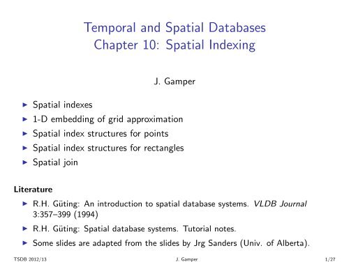
◮ <strong>Spatial</strong> indexes<br />
<strong>Temporal</strong> <strong>and</strong> <strong>Spatial</strong> <strong>Databases</strong><br />
<strong>Chapter</strong> <strong>10</strong>: <strong>Spatial</strong> <strong>Indexing</strong><br />
J. Gamper<br />
◮ 1-D embedding of grid approximation<br />
◮ <strong>Spatial</strong> index structures for points<br />
◮ <strong>Spatial</strong> index structures for rectangles<br />
◮ <strong>Spatial</strong> join<br />
Literature<br />
◮ R.H. Güting: An introduction to spatial database systems. VLDB Journal<br />
3:357–399 (1994)<br />
◮ R.H. Güting: <strong>Spatial</strong> database systems. Tutorial notes.<br />
◮ Some slides are adapted from the slides by Jrg S<strong>and</strong>ers (Univ. of Alberta).<br />
TSDB 2012/13 J. Gamper 1/27
<strong>Spatial</strong> <strong>Indexing</strong>/1<br />
◮ Conventional index structures such as B-trees are not designed to support<br />
spatial queries<br />
◮ Group objects only along one dimension<br />
◮ Do not preserve spatial proximity<br />
◮ Example: NN Query – Nearest neighbor of Q is typically not the nearest<br />
neighbor in any dimension.<br />
TSDB 2012/13 J. Gamper 2/27
<strong>Spatial</strong> <strong>Indexing</strong>/2<br />
◮ <strong>Spatial</strong> index structures try to preserve spatial proximity<br />
◮ Group objects that are close to each other in space on the same data page<br />
◮ Problem: the number of bytes to store extended spatial objects (lines,<br />
polygons) varies<br />
◮ Solution.<br />
◮ Store approximations of spatial objects in the index structure, typically<br />
axis-parallel minimum bounding rectangles (MBR)<br />
◮ Exact object representation (ER) is stored separately; points to ER in the<br />
index<br />
TSDB 2012/13 J. Gamper 3/27
<strong>Spatial</strong> <strong>Indexing</strong>/3<br />
◮ A fundamental idea of spatial indexing is the use of approximations<br />
◮ Two types of approximations<br />
◮ Continuous approximation, e.g., a bounding box<br />
◮ Grid approximation<br />
◮ The use of approximation leads to a filter <strong>and</strong> refine strategy for query<br />
processing.<br />
TSDB 2012/13 J. Gamper 4/27
<strong>Spatial</strong> <strong>Indexing</strong>/4<br />
Filter <strong>and</strong> refine strategy<br />
1. Filter step:<br />
◮ Use index to find all approximations that satisfy the query<br />
◮ Some objects already satisfy the query based on the approximation, others<br />
have to be checked in the refine step<br />
◮ Returns a set of c<strong>and</strong>idate objects, which is a superset of the objects<br />
fulfilling a predicate<br />
2. Refine step:<br />
◮ Load the exact object representations for the c<strong>and</strong>idates<br />
◮ Test whether the c<strong>and</strong>idates satisfy the query<br />
TSDB 2012/13 J. Gamper 5/27
<strong>Spatial</strong> <strong>Indexing</strong>/5<br />
◮ Mainly used to support spatial selection<br />
◮ but supports also other operations, e.g., spatial join or finding the closest<br />
object<br />
◮ A spatial index organizes space <strong>and</strong> the objects in it in some way so that<br />
only parts of the space <strong>and</strong> a subset of the objects need to be considered to<br />
answer a query<br />
◮ Two main approaches:<br />
◮ Map spatial objects to a 1-D space <strong>and</strong> utilize st<strong>and</strong>ard indexing techniques,<br />
e.g., Z-order + B-tree<br />
◮ Dedicated spatial index data structures<br />
◮ Data organizing, e.g., R-tree<br />
◮ Space organizing, e.g., Quad-tree<br />
TSDB 2012/13 J. Gamper 6/27
<strong>Spatial</strong> <strong>Indexing</strong>/6<br />
◮ Most spatial data structures are designed to either store points (for point<br />
values) or rectangles (for line <strong>and</strong> region values)<br />
◮ Operations on those structures: insert, delete, check membership<br />
◮ Typical query types<br />
◮ for points:<br />
◮ Range query: all points within a query rectangle<br />
◮ Nearest neighbor: point closest to a query point<br />
◮ Distance scan: enumerate points in increasing distance from a query point<br />
◮ for rectangles:<br />
◮ Intersection query<br />
◮ Containment query<br />
TSDB 2012/13 J. Gamper 7/27
1-D Embedding of Grid Approximation/1<br />
◮ Basic idea of 1-D embedding of grid approximation<br />
1. The data space is partitioned into rectangular cells (a grid)<br />
2. Find a linear order for the cells of the grid such that cells close together in<br />
space are also close to each other in the linear order; assign a number to<br />
each cell<br />
◮ The order should maintain locality/proximity<br />
◮ The order should be easily to compute<br />
◮ Space filling curves are used for that<br />
3. Define this order recursively for a grid that is obtained by a hierarchical<br />
subdivision of space<br />
4. Objects are approximated by cells<br />
5. Store the cell numbers for objects in a conventional index structure with<br />
respect to the linear order<br />
TSDB 2012/13 J. Gamper 8/27
1-D Embedding of Grid Approximation/2<br />
Example: Space filling curves<br />
TSDB 2012/13 J. Gamper 9/27
1-D Embedding of Grid Approximation/3<br />
◮ Z-Order is the most popular such order (Morton 1966, Orenstein <strong>and</strong><br />
Manola, 1988)<br />
◮ Also termed Morton order or bit-interleaving<br />
◮ Each cell at each level of the hierarchy has an associated bit string whose<br />
length corresponds to the level to which the cell belongs.<br />
◮ e.g., the top-right cell in the left diagram has bit string 11, on the right-side<br />
cell 11<strong>10</strong> is shown.<br />
◮ The bit-string 11<strong>10</strong> is obtained by choosing 11 at the top level, <strong>and</strong> then <strong>10</strong><br />
within the top level quadrant.<br />
◮ The order which is imposed on all cells of a hierarchical subdivision is given<br />
by the lexicographical order of the bit strings.<br />
TSDB 2012/13 J. Gamper <strong>10</strong>/27
1-D Embedding of Grid Approximation/4<br />
◮ Any shape (approximated as a set of cells) over the grid can now be<br />
decomposed into a minimal number of cells at different levels (always<br />
using the highest possible level).<br />
◮ It can therefore be represented by a set of bit strings, called z-elements<br />
◮ For a spatial object, the corresponding set of z-elements builds a set of<br />
spatial keys<br />
◮ <strong>Spatial</strong> index: Put z-elements as spatial keys in lexicographical order into<br />
a B-tree.<br />
◮ Due to the proximity-preserving property various types of queries can be<br />
answered relatively efficiently, e.g., containment or range query with<br />
rectangle r<br />
◮ determine z-elements of r<br />
◮ for each z-element z scan a part of the leaf sequence of the B-tree having z<br />
as prefix.<br />
◮ Check these c<strong>and</strong>idates for actual containment.<br />
TSDB 2012/13 J. Gamper 11/27
1-D Embedding of Grid Approximation/5<br />
Example: Mapping 1D-embedding to a B+-tree<br />
◮ Key values (c,l) in the nodes represent the decimal representation of the<br />
cell number <strong>and</strong> the level.<br />
TSDB 2012/13 J. Gamper 12/27
<strong>Spatial</strong> Index Structures<br />
◮ A (dedicated) spatial index structure organizes objects into buckets<br />
◮ Each bucket has an associated bucket region, a part of space containing<br />
all objects stored in that bucket.<br />
◮ For point data structures, the regions are disjoint<br />
◮ the space is partitioned <strong>and</strong> each point belongs to precisely one bucket<br />
◮ e.g., a kd-tree paritioning of 2d-space where each bucket can hold up to 3<br />
points<br />
◮ For rectangle data structures the bucket regions may overlap<br />
TSDB 2012/13 J. Gamper 13/27
<strong>Spatial</strong> Index Structures for Points/1<br />
◮ <strong>Spatial</strong> index structures for points<br />
◮ Data structures of representing points in k dimensions (multi-attribute)<br />
have a long tradition, e.g., a tuple t = (x1,...,xk)<br />
◮ Can be used to store geometrical points<br />
◮ GRID index: <strong>Spatial</strong> index structure for points (Nievergelt, Hinterberger,<br />
<strong>and</strong> Sevcik 84)<br />
◮ The following example partitions the data space into cells by an irregular grid<br />
◮ The directory is a k-dimensional array whose entries are logical pointers to<br />
buckets.<br />
◮ All points in a cell are stored in the bucket pointed to by the correpsonding<br />
directory entry.<br />
◮ The scales are small <strong>and</strong> are kept in main memory; the directory is on the<br />
disk.<br />
TSDB 2012/13 J. Gamper 14/27
<strong>Spatial</strong> Index Structures for Points/2<br />
◮ kd-Tree (Bentley 75)<br />
◮ Binary tree where each internal node contains a key drawn from one of the<br />
k dimensions<br />
◮ The key in the root node (level 0) divides the data space with respect to<br />
dimension 0, the keys in its sons (level 1) divide the two subspaces with<br />
repsect to dimension 1, <strong>and</strong> so forth, up to dimension k −1, after which<br />
cycling through the dimensions restarts.<br />
◮ Leaves contain the points to be stored<br />
◮ KDB-tree (Robinson 81): introduce buckets, paginate the binary tree, all<br />
leaves at the same level (like B-tree)<br />
◮ LSD-tree (Henrich et al. 89): ab<strong>and</strong>on strict cycling through dimensions;<br />
clever paging algorithm keeps external path length balanced even for very<br />
unbalanced binary trees.<br />
TSDB 2012/13 J. Gamper 15/27
<strong>Spatial</strong> Index Structures for Points/3<br />
◮ Quad-Tree<br />
◮ Class of spatial index structures which divide the data space recursively into<br />
4 quadrants (NW, NE, SW, SE)<br />
TSDB 2012/13 J. Gamper 16/27
<strong>Spatial</strong> Index Structures for Points/4<br />
◮ Quad-Tree (contd.)<br />
◮ Different algorithms for quad-trees for processing points, lines, plygons (i.e.,<br />
different node types, construction <strong>and</strong> query algorithms)<br />
◮ Frequently used in commercial GIS especially for compressing, storing <strong>and</strong><br />
manipulating of raster images<br />
TSDB 2012/13 J. Gamper 17/27
<strong>Spatial</strong> Index Structures for Rectangles/1<br />
◮ <strong>Spatial</strong> index structures for rectangles<br />
◮ Unlike points, rectangles do not fall into a unique cell of a partition <strong>and</strong><br />
might intersect partition boundaries<br />
◮ Three main approaches:<br />
◮ Transformation approach<br />
◮ Overlapping bucket regions<br />
◮ Clipping<br />
TSDB 2012/13 J. Gamper 18/27
<strong>Spatial</strong> Index Structures for Rectangles/2<br />
◮ Transformation approach<br />
◮ k-dimensional rectangles are transformed into 2k-dimensional points, <strong>and</strong> a<br />
point data structure is used.<br />
◮ Rectangle (xl,xr,yb,yt) can be viewed as a point in 4-D space<br />
◮ Example: Interval i = (i1,i2) is mapped into a point (x,y) in 2-D space<br />
◮ An intersection query with an interval q = (q1,q2) translates to a condition:<br />
Find all points (x ′ ,y ′ ) s.t. x ′ < q2 <strong>and</strong> y ′ > q1.<br />
◮ All intervals instersecting q are in the shaded area<br />
TSDB 2012/13 J. Gamper 19/27
<strong>Spatial</strong> Index Structures for Rectangles/3<br />
◮ Overlapping bucket regions<br />
◮ Partitioning space is ab<strong>and</strong>oned <strong>and</strong> bucket regions may overlap, e.g.,<br />
R-tree (Guttmann 84)<br />
◮ Advantage: <strong>Spatial</strong> object (or key) is in a single bucket<br />
◮ Disadvantage: Multiple search paths due to overlapping bucket regions<br />
TSDB 2012/13 J. Gamper 20/27
<strong>Spatial</strong> Index Structures for Rectangles/4<br />
◮ Clipping<br />
◮ Bucket regions are disjoint, but data rectangles are cut into several pieces (if<br />
necessary), e.g., R + -tree (Sellis, Rossopoulos <strong>and</strong> Faloutsos 87)<br />
◮ Advantage: Less branching in search<br />
◮ Disadvantage: Multiple entries for a single spatial object<br />
TSDB 2012/13 J. Gamper 21/27
Basic <strong>Spatial</strong> Queries<br />
◮ Containment Query: Given a<br />
spatial object R, find all objects<br />
that completely contain R. If R is<br />
a point, then it is a point query.<br />
◮ Region Query: Given a region R<br />
(polygon or circle), find all spatial<br />
objects that intersect with R. If R<br />
is a rectanlge, then it is a window<br />
query.<br />
◮ Enclosure Query: Given a plygon<br />
region R, find all objects that are<br />
completely contained in R.<br />
◮ K-nearest neighbor Query:<br />
Given an object P, find the k4<br />
objects that are closest to P<br />
(typically for points)<br />
TSDB 2012/13 J. Gamper 22/27
<strong>Spatial</strong> Join/1<br />
◮ Given two sets of spatial objects (typically minimum bounding rectangles)<br />
S1 = {R1,...,Rm},S2 = {R ′ 1,...,R ′ n}<br />
◮ Determine for S1 <strong>and</strong> S2 all object pairs that are in a relationship described<br />
by a spatial predicate (typically intersection, but other predicates are also<br />
possible)<br />
TSDB 2012/13 J. Gamper 23/27
<strong>Spatial</strong> Join/2<br />
◮ Very active research area in the last few years<br />
◮ Traditional join methods such as hash join or sort/merge join are not<br />
applicable<br />
◮ Filtering Cartesian product is expensive<br />
◮ Central ideas<br />
◮ filter + refine<br />
◮ use of spatial index structures<br />
◮ Classification of strategies<br />
◮ Grid approximation/bounding box<br />
◮ None/one/both oper<strong>and</strong>s are represented in a spatial index structure<br />
TSDB 2012/13 J. Gamper 24/27
<strong>Spatial</strong> Join/3<br />
◮ Grid approximations with<br />
an overlap predicate<br />
◮ A parallel scan of two<br />
sets of z-elements<br />
corresponding to two<br />
sets of spatial objects is<br />
performed<br />
◮ Similar to a merge join<br />
TSDB 2012/13 J. Gamper 25/27
<strong>Spatial</strong> Join/4<br />
◮ Bounding box approximation: For two sets of rectangles R <strong>and</strong> S all<br />
pairs (r,s), r ∈ R <strong>and</strong> s ∈ S such that r intersects s:<br />
◮ No spatial index on R <strong>and</strong> S: bb join algorithm uses a computational<br />
geometry algorithm to detect rectangle intersection, similar to external<br />
merge sorting<br />
◮ <strong>Spatial</strong> index on either R or S: index join scans the non-indexed oper<strong>and</strong><br />
<strong>and</strong> for each object, the bounding box of its SDT attribute is used as a<br />
search argument on the indexed oper<strong>and</strong> (only efficient if non-indexed<br />
oper<strong>and</strong> is not too big)<br />
◮ Both R <strong>and</strong> S are indexed: synchronized traversal of both structures so that<br />
pairs of cells of their repsective partitions covering the same part of space<br />
are encountered together.<br />
TSDB 2012/13 J. Gamper 26/27
Summary<br />
◮ <strong>Spatial</strong> indexes are a crucial part of any database systems that supports<br />
geographical information.<br />
◮ <strong>Spatial</strong> indexing techniques are necessary to efficiently answer queries.<br />
◮ Mapping to lower dimensional space, grid file, kd tree, family of R-tree<br />
indexes<br />
TSDB 2012/13 J. Gamper 27/27