Improvements of the Lucas-Kanade Optical-Flow Algorithm
Improvements of the Lucas-Kanade Optical-Flow Algorithm
Improvements of the Lucas-Kanade Optical-Flow Algorithm

Create successful ePaper yourself
Turn your PDF publications into a flip-book with our unique Google optimized e-Paper software.
<strong>Improvements</strong> <strong>of</strong> <strong>the</strong> <strong>Lucas</strong>-<strong>Kanade</strong> <strong>Optical</strong>-<strong>Flow</strong> <strong>Algorithm</strong><br />
An Improvement <strong>of</strong> <strong>the</strong> <strong>Lucas</strong>-<strong>Kanade</strong> <strong>Optical</strong>-<strong>Flow</strong><br />
<strong>Algorithm</strong> for every Circumstance<br />
Lorenz Gerstmayr<br />
Computer Engineering Group<br />
Faculty <strong>of</strong> Technology<br />
University <strong>of</strong> Bielefeld<br />
2008-06-11<br />
Corrected version: 2008-08-05
<strong>Improvements</strong> <strong>of</strong> <strong>the</strong> <strong>Lucas</strong>-<strong>Kanade</strong> <strong>Optical</strong>-<strong>Flow</strong> <strong>Algorithm</strong><br />
Today’s talk<br />
1 Basics about optical flow<br />
2 Standard <strong>Lucas</strong>-<strong>Kanade</strong> method<br />
3 <strong>Improvements</strong><br />
4 Discussion
<strong>Improvements</strong> <strong>of</strong> <strong>the</strong> <strong>Lucas</strong>-<strong>Kanade</strong> <strong>Optical</strong>-<strong>Flow</strong> <strong>Algorithm</strong><br />
Basics about optical flow<br />
Definition<br />
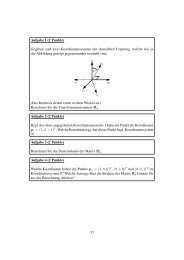
Definition <strong>of</strong> optical flow<br />
Definiton<br />
P ′ (1)<br />
u<br />
Nodal point<br />
P(1) P(2) ∈ R 3<br />
P ′ (2) ∈ R 2<br />
Image<br />
Example<br />
http://www.ezls.fb12.uni-siegen.de/lehre/WebOne/index.htm
<strong>Improvements</strong> <strong>of</strong> <strong>the</strong> <strong>Lucas</strong>-<strong>Kanade</strong> <strong>Optical</strong>-<strong>Flow</strong> <strong>Algorithm</strong><br />
Basics about optical flow<br />
Definition<br />
Image Brightness Constancy Constraint (IBCC)<br />
B:<br />
A:<br />
Image brightness constancy constraint:<br />
A(p + u(p)) = B(p)
<strong>Improvements</strong> <strong>of</strong> <strong>the</strong> <strong>Lucas</strong>-<strong>Kanade</strong> <strong>Optical</strong>-<strong>Flow</strong> <strong>Algorithm</strong><br />
Basics about optical flow<br />
Common problems<br />
Common problems<br />
Aperture problem Correspondence problem<br />
After: B. Jähne, Dig. Img. Proc., 2000
<strong>Improvements</strong> <strong>of</strong> <strong>the</strong> <strong>Lucas</strong>-<strong>Kanade</strong> <strong>Optical</strong>-<strong>Flow</strong> <strong>Algorithm</strong><br />
Standard <strong>Lucas</strong>-<strong>Kanade</strong> method<br />
Basics<br />
Optic flow equation<br />
Image brightness constancy constraint:<br />
Optic flow equation:<br />
A(p + u(p)) = B(p)<br />
First order Taylor approximation (with u = [ux, uy] ⊤ ):<br />
A(p) + Ax(p)ux(p) + Ay(p)uy(p) = B(p)<br />
<br />
A + [Ax, Ay]<br />
<br />
ux<br />
[Ax, Ay]<br />
uy<br />
ux<br />
uy<br />
+ (A − B)<br />
<br />
At<br />
= B<br />
= 0<br />
B. Jähne, Dig. Img. Proc., 2000; B.D. <strong>Lucas</strong> & T. <strong>Kanade</strong>, Proc. Im. Underst. Workshop, 1981
<strong>Improvements</strong> <strong>of</strong> <strong>the</strong> <strong>Lucas</strong>-<strong>Kanade</strong> <strong>Optical</strong>-<strong>Flow</strong> <strong>Algorithm</strong><br />
Standard <strong>Lucas</strong>-<strong>Kanade</strong> method<br />
Derivation<br />
Derivation<br />
Optic flow equation:<br />
<br />
ux<br />
[Ax, Ay] + At = 0<br />
uy<br />
Underdetermined problem (aperture problem)<br />
Approach:<br />
Assuming optical flow to be locally constant<br />
Weighting w.r.t. distance to center pixel p <strong>of</strong> image patch Ω:<br />
e(u) = <br />
w 2 <br />
<br />
ux(x)<br />
(x) [Ax(x), Bx(x)] + At(x)<br />
uy(x)<br />
x∈Ω<br />
2<br />
!<br />
= min<br />
B. Jähne, Dig. Img. Proc., 2000; B.D. <strong>Lucas</strong> & T. <strong>Kanade</strong>, Proc. Im. Underst. Workshop, 1981
<strong>Improvements</strong> <strong>of</strong> <strong>the</strong> <strong>Lucas</strong>-<strong>Kanade</strong> <strong>Optical</strong>-<strong>Flow</strong> <strong>Algorithm</strong><br />
Standard <strong>Lucas</strong>-<strong>Kanade</strong> method<br />
Derivation<br />
Derivation<br />
Weighted least squares approach<br />
e(u) = <br />
w<br />
x∈Ω<br />
2<br />
2 ux<br />
!<br />
[Ax, Ay] + At = min<br />
uy<br />
Partial derivatives:<br />
∂e<br />
= 2<br />
∂ux<br />
<br />
w<br />
x∈Ω<br />
2<br />
<br />
ux<br />
[Ax, Ay] + At Ax<br />
uy<br />
! = min<br />
∂e<br />
= 2<br />
∂uy<br />
<br />
w<br />
x∈Ω<br />
2<br />
<br />
ux<br />
[Ax, Ay] + At Ay<br />
uy<br />
! = min<br />
B. Jähne, Dig. Img. Proc., 2000; B.D. <strong>Lucas</strong> & T. <strong>Kanade</strong>, Proc. Im. Underst. Workshop, 1981
<strong>Improvements</strong> <strong>of</strong> <strong>the</strong> <strong>Lucas</strong>-<strong>Kanade</strong> <strong>Optical</strong>-<strong>Flow</strong> <strong>Algorithm</strong><br />
Standard <strong>Lucas</strong>-<strong>Kanade</strong> method<br />
Derivation<br />
Derivation<br />
Weighted least squares approach:<br />
Sorting:<br />
∂e<br />
= 2<br />
∂ux<br />
<br />
w<br />
x∈Ω<br />
2<br />
<br />
ux<br />
[Ax, Ay] + At Ax<br />
uy<br />
! = min<br />
∂e<br />
= 2<br />
∂uy<br />
<br />
w<br />
x∈Ω<br />
2<br />
<br />
ux<br />
[Ax, Ay] + At Ay<br />
uy<br />
! = min<br />
<br />
<br />
〈AxAx〉 〈AxAy〉 ux 〈AxAt〉<br />
= −<br />
〈AxAy〉 〈AyAy〉 uy 〈AyAt〉<br />
<br />
G<br />
b<br />
〈a〉 = <br />
w 2 (x)a(x)<br />
x∈Ω
<strong>Improvements</strong> <strong>of</strong> <strong>the</strong> <strong>Lucas</strong>-<strong>Kanade</strong> <strong>Optical</strong>-<strong>Flow</strong> <strong>Algorithm</strong><br />
Standard <strong>Lucas</strong>-<strong>Kanade</strong> method<br />
Derivation<br />
Solution<br />
Weighted least squares approach:<br />
Aperture problem<br />
Eigenvalues λ1, λ2 <strong>of</strong> G:<br />
Gu = b<br />
u = G −1 b<br />
λ1, λ2 > 0 λ1 > 0, λ2 ≈ 0 λ1, λ2 ≈ 0<br />
B. Jähne, Dig. Img. Proc., 2000; B.D. <strong>Lucas</strong> & T. <strong>Kanade</strong>, Proc. Im. Underst. Workshop, 1981
<strong>Improvements</strong> <strong>of</strong> <strong>the</strong> <strong>Lucas</strong>-<strong>Kanade</strong> <strong>Optical</strong>-<strong>Flow</strong> <strong>Algorithm</strong><br />
Standard <strong>Lucas</strong>-<strong>Kanade</strong> method<br />
Limitations and restrictions<br />
Limitations and possible improvements<br />
Standard LK<br />
Iterated LK<br />
Multiscale LK<br />
baseline<br />
most efficient<br />
more<br />
accurate<br />
large<br />
displacements<br />
Illumination Tolerance<br />
illumination<br />
changes<br />
LK with flowfield constraints<br />
Global LK<br />
types <strong>of</strong><br />
flowfields<br />
global flow<br />
computation
<strong>Improvements</strong> <strong>of</strong> <strong>the</strong> <strong>Lucas</strong>-<strong>Kanade</strong> <strong>Optical</strong>-<strong>Flow</strong> <strong>Algorithm</strong><br />
<strong>Improvements</strong><br />
Iterated <strong>Lucas</strong>-<strong>Kanade</strong> algorithm<br />
Motivation<br />
Sketch Motivation<br />
Deviations due to first order<br />
approximation<br />
Large displacements within<br />
aperture<br />
Iteratively refine <strong>the</strong> flow vector<br />
Improvement:<br />
More accurate flow estimates<br />
J.Y. Bouguet, Tech. Report, Intel Cooperation, 2000
<strong>Improvements</strong> <strong>of</strong> <strong>the</strong> <strong>Lucas</strong>-<strong>Kanade</strong> <strong>Optical</strong>-<strong>Flow</strong> <strong>Algorithm</strong><br />
<strong>Improvements</strong><br />
Iterated <strong>Lucas</strong>-<strong>Kanade</strong> algorithm<br />
Derivation<br />
Image brightness constancy constraint:<br />
Refined IBCC:<br />
A(p + u(p)) = B(p)<br />
A(p + u (κ−1) (p) + t (κ) (p)) = B(p)<br />
Iterations 1 ≤ κ ≤ k<br />
Recursion: u (κ) from u (κ−1) and t (κ)<br />
Initial estimate: u 0 = 0<br />
Sketch<br />
J.Y. Bouguet, Tech. Report, Intel Cooperation, 2000
<strong>Improvements</strong> <strong>of</strong> <strong>the</strong> <strong>Lucas</strong>-<strong>Kanade</strong> <strong>Optical</strong>-<strong>Flow</strong> <strong>Algorithm</strong><br />
<strong>Improvements</strong><br />
Iterated <strong>Lucas</strong>-<strong>Kanade</strong> algorithm<br />
Derivation<br />
Weighted least squares approach<br />
<br />
(κ)<br />
e t (κ)<br />
= <br />
w<br />
x∈Ω<br />
2 ⎛ ⎛<br />
(x) ⎝A ⎝x + u (κ−1)<br />
+t<br />
<br />
η<br />
(κ)<br />
⎞ ⎞2<br />
⎠ − B(x) ⎠<br />
e(t) = <br />
w 2 (A (η + t) − B) 2<br />
x∈Ω<br />
Taylor-approximation <strong>of</strong> A(η + t) (omitting x):<br />
= <br />
w<br />
x∈Ω<br />
2<br />
⎛<br />
<br />
⎜<br />
tx<br />
⎜<br />
⎝A(η) − B + [Ax(η), Ay(η)]<br />
<br />
ty<br />
At(η)<br />
⎞2<br />
⎟<br />
⎠<br />
!<br />
= 0
<strong>Improvements</strong> <strong>of</strong> <strong>the</strong> <strong>Lucas</strong>-<strong>Kanade</strong> <strong>Optical</strong>-<strong>Flow</strong> <strong>Algorithm</strong><br />
<strong>Improvements</strong><br />
Iterated <strong>Lucas</strong>-<strong>Kanade</strong> algorithm<br />
Derivation<br />
Weighted least squares approach<br />
e(t) = <br />
w<br />
x∈Ω<br />
2<br />
<br />
2 tx<br />
At(η) + [Ax(η), Ay(η)]<br />
ty<br />
Partial derivatives:<br />
<br />
∂e<br />
,<br />
∂tx<br />
∂e<br />
⊤ = 2<br />
∂ty<br />
<br />
w<br />
x∈Ω<br />
2<br />
<br />
<br />
tx Ax(η)<br />
At(η) + [Ax(η), Ay(η)]<br />
ty Ay(η)<br />
Solution (with η = x + u (κ−1) ):<br />
<br />
<br />
<br />
〈Ax(η)Ax(η)〉 〈Ax(η)Ay(η)〉 tx 〈Ax(η)At(η)〉<br />
= −<br />
〈Ax(η)Ay(η)〉 〈Ay(η)Ay(η)〉 ty 〈Ay(η)At(η)〉
<strong>Improvements</strong> <strong>of</strong> <strong>the</strong> <strong>Lucas</strong>-<strong>Kanade</strong> <strong>Optical</strong>-<strong>Flow</strong> <strong>Algorithm</strong><br />
<strong>Improvements</strong><br />
Iterated <strong>Lucas</strong>-<strong>Kanade</strong> algorithm<br />
Simplified solution<br />
Solution<br />
<br />
<br />
<br />
〈Ax(η)Ax(η)〉 〈Ax(η)Ay(η)〉 tx 〈Ax(η)At(η)〉<br />
= −<br />
〈Ax(η)Ay(η)〉 〈Ay(η)Ay(η)〉 ty 〈Ay(η)At(η)〉<br />
<br />
=G(η)<br />
=b(η)<br />
Problem<br />
G depends on η = x + u (κ−1)<br />
⇒ Recomputation <strong>of</strong> G −1 needed for each iteration<br />
A and B contain identical gradient information<br />
Compute Bx and By instead <strong>of</strong> Ax and Ay<br />
J.Y. Bouguet, Tech. Report, Intel Cooperation, 2000
<strong>Improvements</strong> <strong>of</strong> <strong>the</strong> <strong>Lucas</strong>-<strong>Kanade</strong> <strong>Optical</strong>-<strong>Flow</strong> <strong>Algorithm</strong><br />
<strong>Improvements</strong><br />
Iterated <strong>Lucas</strong>-<strong>Kanade</strong> algorithm<br />
Simplified solution<br />
Solution<br />
<br />
<br />
<br />
〈Ax(η)Ax(η)〉 〈Ax(η)Ay(η)〉 tx 〈Ax(η)At(η)〉<br />
= −<br />
〈Ax(η)Ay(η)〉 〈Ay(η)Ay(η)〉 ty 〈Ay(η)At(η)〉<br />
<br />
=G(η)<br />
=b(η)<br />
Simplified solution<br />
<br />
<br />
〈BxBx〉 〈BxBy〉 tx 〈BxAt(η)〉<br />
= −<br />
〈BxBy〉 〈ByBy〉 ty 〈ByAt(η)〉<br />
<br />
=G<br />
=b(η)<br />
J.Y. Bouguet, Tech. Report, Intel Cooperation, 2000
<strong>Improvements</strong> <strong>of</strong> <strong>the</strong> <strong>Lucas</strong>-<strong>Kanade</strong> <strong>Optical</strong>-<strong>Flow</strong> <strong>Algorithm</strong><br />
<strong>Improvements</strong><br />
Iterated <strong>Lucas</strong>-<strong>Kanade</strong> algorithm<br />
Building blocks<br />
Refinement vector<br />
Image mismatch vector<br />
Temporal derivative<br />
Recursion<br />
b (κ) = −<br />
t (κ) = G −1 b (κ)<br />
A (κ)<br />
t = B(p) − A<br />
<br />
〈BxA (κ)<br />
t 〉, 〈ByA (κ)<br />
⊤ t 〉<br />
<br />
p + u (κ−1)<br />
u (κ) = u (κ−1) + t (κ)
<strong>Improvements</strong> <strong>of</strong> <strong>the</strong> <strong>Lucas</strong>-<strong>Kanade</strong> <strong>Optical</strong>-<strong>Flow</strong> <strong>Algorithm</strong><br />
<strong>Improvements</strong><br />
Multiscale <strong>Lucas</strong>-<strong>Kanade</strong> algorithm<br />
Motivation<br />
Sketch Motivation and approach<br />
Improvement<br />
Applicable for large image displacements<br />
IBCC and Taylor only valid for<br />
small movements<br />
Larger displacements are common<br />
Multi-scale approach<br />
Coarse-to-fine propagation<br />
Identical aperture sizes<br />
but shifted center position<br />
J.Y. Bouguet, Tech. Report, Intel Cooperation, 2000
<strong>Improvements</strong> <strong>of</strong> <strong>the</strong> <strong>Lucas</strong>-<strong>Kanade</strong> <strong>Optical</strong>-<strong>Flow</strong> <strong>Algorithm</strong><br />
<strong>Improvements</strong><br />
Multiscale <strong>Lucas</strong>-<strong>Kanade</strong> algorithm<br />
Gaussian image pyramid<br />
Theory<br />
Pyramidal images: I (κ)<br />
Pixel positions: p (κ) = 1<br />
2 κ p<br />
coarse<br />
fine<br />
λ = ℓ − 1<br />
λ = 2<br />
λ = 1<br />
λ = 0
<strong>Improvements</strong> <strong>of</strong> <strong>the</strong> <strong>Lucas</strong>-<strong>Kanade</strong> <strong>Optical</strong>-<strong>Flow</strong> <strong>Algorithm</strong><br />
<strong>Improvements</strong><br />
Multiscale <strong>Lucas</strong>-<strong>Kanade</strong> algorithm<br />
Gaussian image pyramid<br />
Theory<br />
Pyramidal images: I (κ)<br />
Pixel positions: p (κ) = 1<br />
2 κ p<br />
coarse<br />
fine<br />
λ = ℓ − 1<br />
λ = 2<br />
λ = 1<br />
λ = 0<br />
Example<br />
fine ↔ coarse<br />
http://www.prip.tuwien.ac.at/research/research-areas/image-pyramids/
<strong>Improvements</strong> <strong>of</strong> <strong>the</strong> <strong>Lucas</strong>-<strong>Kanade</strong> <strong>Optical</strong>-<strong>Flow</strong> <strong>Algorithm</strong><br />
<strong>Improvements</strong><br />
Multiscale <strong>Lucas</strong>-<strong>Kanade</strong> algorithm<br />
<strong>Algorithm</strong><br />
Input:<br />
Two image pyramides A (λ) and B (λ) , 0 ≤ λ ≤ ℓ − 1<br />
Coarse-to-fine recursion (at level λ)<br />
<strong>Flow</strong> estimate u (λ) is given (initial estimate: u (ℓ−1) = 0)<br />
Compute refinement vector t (λ) :<br />
<br />
e t (λ)<br />
= <br />
x∈Ω<br />
Propagation to finer level λ − 1:<br />
<br />
2<br />
w(x) A x + u (λ) + t (λ)<br />
2 − B(x)<br />
u (λ−1) <br />
= 2 u (λ) + t (λ)<br />
J.Y. Bouguet, Tech. Report, Intel Cooperation, 2000
<strong>Improvements</strong> <strong>of</strong> <strong>the</strong> <strong>Lucas</strong>-<strong>Kanade</strong> <strong>Optical</strong>-<strong>Flow</strong> <strong>Algorithm</strong><br />
<strong>Improvements</strong><br />
Tolerance against illumination changes<br />
Motivation<br />
Sketch<br />
Improvement<br />
Tolerance against<br />
illumination changes<br />
IBCC<br />
Refined IBCC<br />
A(p + u(p)) = B(p)<br />
A(p + u(p)) = α(p)B(p) + β(p)<br />
Brigthness change model<br />
Linear gray value changes<br />
α and β locally constant<br />
Compute t = [ux, uy, α, β] ⊤<br />
S. Negahdaripour, IEEE PAMI, 1998; H.W. Haussecker & D.J. Fleet, Proc. CVPR, 2000;<br />
Y. Altunbasak et.al., IEEE TIP, 2003; Y.H. Kim et.al., Img. Vis. Comp., 2005
<strong>Improvements</strong> <strong>of</strong> <strong>the</strong> <strong>Lucas</strong>-<strong>Kanade</strong> <strong>Optical</strong>-<strong>Flow</strong> <strong>Algorithm</strong><br />
<strong>Improvements</strong><br />
Tolerance against illumination changes<br />
Derivation<br />
Error function (omitting x)<br />
e(t) = <br />
w 2<br />
<br />
[Ax, Ay] ⊤<br />
<br />
x∈Ω<br />
<br />
ux<br />
uy<br />
+ A − αB − β<br />
2<br />
S. Negahdaripour, IEEE PAMI, 1998
<strong>Improvements</strong> <strong>of</strong> <strong>the</strong> <strong>Lucas</strong>-<strong>Kanade</strong> <strong>Optical</strong>-<strong>Flow</strong> <strong>Algorithm</strong><br />
<strong>Improvements</strong><br />
Tolerance against illumination changes<br />
Derivation<br />
Partial derivatives (omitting x)<br />
∂e<br />
= 2<br />
∂ux<br />
<br />
w<br />
x∈Ω<br />
2<br />
<br />
[Ax, Ay] ⊤<br />
<br />
<br />
ux<br />
+ A − αB − β Ax<br />
uy<br />
∂e<br />
= 2<br />
∂uy<br />
<br />
w<br />
x∈Ω<br />
2<br />
<br />
[Ax, Ay] ⊤<br />
<br />
<br />
ux<br />
+ A − αB − β Ay<br />
uy<br />
∂e <br />
= −2 w<br />
∂α<br />
x∈Ω<br />
2<br />
<br />
[Ax, Ay] ⊤<br />
<br />
<br />
ux<br />
+ A − αB − β B<br />
uy<br />
∂e <br />
= −2 w<br />
∂β<br />
x∈Ω<br />
2<br />
<br />
[Ax, Ay] ⊤<br />
<br />
<br />
ux<br />
+ A − αB − β<br />
uy<br />
S. Negahdaripour, IEEE PAMI, 1998
<strong>Improvements</strong> <strong>of</strong> <strong>the</strong> <strong>Lucas</strong>-<strong>Kanade</strong> <strong>Optical</strong>-<strong>Flow</strong> <strong>Algorithm</strong><br />
<strong>Improvements</strong><br />
Tolerance against illumination changes<br />
Solution<br />
Error function (omitting x)<br />
e(t) = <br />
w 2<br />
<br />
[Ax, Ay] ⊤<br />
<br />
Solution<br />
x∈Ω<br />
<br />
ux<br />
uy<br />
+ A − αB − β<br />
t = G −1 b<br />
⎛ ⎞<br />
ux<br />
⎜ ⎟<br />
⎜uy<br />
⎟<br />
⎜ ⎟<br />
⎝ α ⎠<br />
β<br />
=<br />
⎛<br />
〈AxAx〉<br />
⎜ 〈AxAy〉<br />
⎜<br />
⎝〈−AxB〉<br />
〈AxAy〉<br />
〈AyAy〉<br />
〈−AyB〉<br />
〈−AxB〉<br />
〈−AyB〉<br />
〈BB〉<br />
⎞−1<br />
〈−Ax〉<br />
〈−Ay〉<br />
⎟<br />
〈B〉 ⎠<br />
〈−Ax〉 〈−Ay〉 〈B〉 〈−1〉<br />
⎛ ⎞<br />
〈−AxA〉<br />
⎜<br />
⎜〈−AyA〉<br />
⎟<br />
⎜ ⎟<br />
⎝ 〈AB〉 ⎠<br />
〈−A〉<br />
2<br />
S. Negahdaripour, IEEE PAMI, 1998
<strong>Improvements</strong> <strong>of</strong> <strong>the</strong> <strong>Lucas</strong>-<strong>Kanade</strong> <strong>Optical</strong>-<strong>Flow</strong> <strong>Algorithm</strong><br />
<strong>Improvements</strong><br />
Tolerance against illumination changes<br />
Discussion<br />
Properties <strong>of</strong> G<br />
Full rank → invertible<br />
Ill-conditioned<br />
Areas <strong>of</strong> weak/regular texture<br />
Multiple interpretations <strong>of</strong> motion and illuminance<br />
Radiometric cues α and β<br />
Discontinuous at motion boundaries or occlusions<br />
⇒ errouneous estimates<br />
⇒ large residuals<br />
Physical interpretations possible:<br />
e.g. irradiance, surface normals, reflectance<br />
S. Negahdaripour, IEEE PAMI, 1998; H.W. Haussecker & D.J. Fleet, Proc. CVPR, 2000
<strong>Improvements</strong> <strong>of</strong> <strong>the</strong> <strong>Lucas</strong>-<strong>Kanade</strong> <strong>Optical</strong>-<strong>Flow</strong> <strong>Algorithm</strong><br />
<strong>Improvements</strong><br />
Movement constraints<br />
Motivation<br />
Motivation<br />
Known camera motion<br />
Approach<br />
Known object motion<br />
<strong>Flow</strong>field “patterns”<br />
Parameterize <strong>the</strong> flowfields:<br />
Solve for a<br />
u(x) = f(x, a)<br />
<strong>Improvements</strong><br />
More accurate flow fields<br />
Uses available knowledge<br />
about flow fields<br />
Derive motion parameters<br />
<strong>Flow</strong>field segmentation
<strong>Improvements</strong> <strong>of</strong> <strong>the</strong> <strong>Lucas</strong>-<strong>Kanade</strong> <strong>Optical</strong>-<strong>Flow</strong> <strong>Algorithm</strong><br />
<strong>Improvements</strong><br />
Movement constraints<br />
Motivation<br />
Motivation<br />
Known camera motion<br />
Approach<br />
Known object motion<br />
<strong>Flow</strong>field “patterns”<br />
Parameterize <strong>the</strong> flowfields:<br />
Solve for a<br />
u(x) = f(x, a)<br />
Example: motion segmentation<br />
http://www-bcs.mit.edu/people/jyawang/demos/garden-layer/
<strong>Improvements</strong> <strong>of</strong> <strong>the</strong> <strong>Lucas</strong>-<strong>Kanade</strong> <strong>Optical</strong>-<strong>Flow</strong> <strong>Algorithm</strong><br />
<strong>Improvements</strong><br />
Movement constraints<br />
Motion models<br />
Translational model<br />
Affine model<br />
<br />
ux a1<br />
=<br />
uy a2<br />
<br />
<br />
ux a1x + a2y + a3<br />
=<br />
uy a4x + a5y + a6<br />
Y. Altunbasak et.al., IEEE TIP, 2003
<strong>Improvements</strong> <strong>of</strong> <strong>the</strong> <strong>Lucas</strong>-<strong>Kanade</strong> <strong>Optical</strong>-<strong>Flow</strong> <strong>Algorithm</strong><br />
<strong>Improvements</strong><br />
Movement constraints<br />
Solution<br />
Refined image brightness constancy constraint<br />
A(p + f(p, a)) = B(p)<br />
Example: Taylor approximation for affine model<br />
Properties and discussion<br />
A(p) + Ax(p)(a1px + a2py + a3)<br />
No interesting properties mentioned<br />
+Ay(p)(a4px + a5py + a6) = B(p)<br />
Y. Altunbasak et.al., IEEE TIP, 2003
<strong>Improvements</strong> <strong>of</strong> <strong>the</strong> <strong>Lucas</strong>-<strong>Kanade</strong> <strong>Optical</strong>-<strong>Flow</strong> <strong>Algorithm</strong><br />
<strong>Improvements</strong><br />
From local to global optical flow<br />
Local vs. global optical flow<br />
Local optical flow<br />
“<strong>Lucas</strong>-<strong>Kanade</strong>”<br />
Sparse flow fields<br />
Analytical solution<br />
Parsimonious<br />
Robust against noise<br />
Global optical flow<br />
“Horn-Schunck”<br />
Dense flow fields (fill-in)<br />
Iterative solution<br />
Computationally cheap<br />
Less robust<br />
B.D. <strong>Lucas</strong> & T. <strong>Kanade</strong>, Proc. Im. Underst. Workshop, 1981; B.K.P. Horn & B.G. Schunck, AI, 1981;<br />
A. Bruhn et.al., Proc. DAGM, 2002; A. Bruhn et.al., IJCV, 2005
<strong>Improvements</strong> <strong>of</strong> <strong>the</strong> <strong>Lucas</strong>-<strong>Kanade</strong> <strong>Optical</strong>-<strong>Flow</strong> <strong>Algorithm</strong><br />
<strong>Improvements</strong><br />
From local to global optical flow<br />
Horn-Schunck in a nutshell<br />
Global error functional (omitting x)<br />
⎛<br />
e(u) = ⎜<br />
⎝<br />
x∈Γ<br />
(Axux + Ayuy + At) 2<br />
<br />
+ϕ |∇ux|<br />
<br />
IBCC<br />
2 + |∇uy| 2<br />
⎟<br />
⎠<br />
<br />
Divergence<br />
Smoothness weight ϕ > 0, Γ is <strong>the</strong> whole image<br />
Solution<br />
Compute optimal u which minimizes e(u)<br />
1 Euler-Lagrange mechanism ⇒ system <strong>of</strong> equations<br />
2 Numerical solution (Gauss-Seidel, SOR, . . .)<br />
A. Bruhn et.al., Proc. DAGM, 2002; A. Bruhn et.al., IJCV, 2005<br />
⎞
<strong>Improvements</strong> <strong>of</strong> <strong>the</strong> <strong>Lucas</strong>-<strong>Kanade</strong> <strong>Optical</strong>-<strong>Flow</strong> <strong>Algorithm</strong><br />
<strong>Improvements</strong><br />
From local to global optical flow<br />
<strong>Lucas</strong>-<strong>Kanade</strong> meets Horn-Schunck<br />
Horn-Schunck error functional<br />
e(u) = <br />
x∈Γ<br />
Combined error functional<br />
<br />
(Axux + Ayuy + At) 2 <br />
+ ϕ |∇ux| 2 + |∇uy| 2<br />
e(u) = <br />
⎛<br />
⎝<br />
x∈Γ<br />
<br />
x ′ w<br />
∈Ω<br />
2<br />
2 ux<br />
[Ax, Ay] + At + . . .<br />
uy<br />
<br />
ϕ |∇ux| 2 + |∇uy| 2<br />
A. Bruhn et.al., Proc. DAGM, 2002; A. Bruhn et.al., IJCV, 2005
<strong>Improvements</strong> <strong>of</strong> <strong>the</strong> <strong>Lucas</strong>-<strong>Kanade</strong> <strong>Optical</strong>-<strong>Flow</strong> <strong>Algorithm</strong><br />
<strong>Improvements</strong><br />
From local to global optical flow<br />
<strong>Lucas</strong>-<strong>Kanade</strong> meets Horn-Schunck<br />
Combined error functional<br />
Euler-Lagrange solutions<br />
e(u) = eLKHS(u) + ϕeR(u)<br />
0 = ∆ux − 1<br />
ϕ (〈AxAx〉ux + 〈AxAy〉uy + 〈AxAt〉)<br />
0 = ∆uy − 1<br />
ϕ (〈AxAy〉ux + 〈AyAy〉uy + 〈AyAt〉)<br />
Laplaceans ∆ux, ∆uy<br />
Discrete approximation<br />
Standard solvers for sparse sets <strong>of</strong> linear equations (SOR)<br />
A. Bruhn et.al., Proc. DAGM, 2002; A. Bruhn et.al., IJCV, 2005
<strong>Improvements</strong> <strong>of</strong> <strong>the</strong> <strong>Lucas</strong>-<strong>Kanade</strong> <strong>Optical</strong>-<strong>Flow</strong> <strong>Algorithm</strong><br />
Discussion<br />
Summary<br />
Limitations and possible improvements<br />
Standard LK<br />
Iterated LK<br />
Multiscale LK<br />
baseline<br />
most efficient<br />
more<br />
accurate<br />
large<br />
displacements<br />
Illumination Tolerance<br />
illumination<br />
changes<br />
LK with flowfield constraints<br />
Global LK<br />
types <strong>of</strong><br />
flowfields<br />
global flow<br />
computation
<strong>Improvements</strong> <strong>of</strong> <strong>the</strong> <strong>Lucas</strong>-<strong>Kanade</strong> <strong>Optical</strong>-<strong>Flow</strong> <strong>Algorithm</strong><br />
Discussion<br />
Summary<br />
Results?!?<br />
Unifying review<br />
Does not exist<br />
Reviewing myself<br />
Different data sets<br />
Unclear parameters<br />
Missing visualizations for parameters<br />
From some papers only a small subset was presented<br />
Quality <strong>of</strong> figures<br />
Benchmarking myself<br />
Availability <strong>of</strong> implementations<br />
Costs and benefits?
<strong>Improvements</strong> <strong>of</strong> <strong>the</strong> <strong>Lucas</strong>-<strong>Kanade</strong> <strong>Optical</strong>-<strong>Flow</strong> <strong>Algorithm</strong><br />
Discussion<br />
Outlook<br />
Relevance for my work<br />
Standard LK<br />
Iterated LK<br />
Multiscale LK<br />
tested<br />
12 ◦ to 15 ◦<br />
tested<br />
8 ◦ to 11 ◦<br />
tested<br />
5 ◦ to 8 ◦<br />
Illumination Tolerance<br />
TODO<br />
LK with flowfield constraints<br />
Global LK<br />
motion seg.?<br />
parameters?<br />
role <strong>of</strong> fill-in<br />
effects?<br />
A. Vardy & R. Möller, Conn. Sci., 2005; L. Gerstmayr, Tech. Report, Uni Bielefeld, 2007