1 Code Generation Code generator phase ... - VTU e-Learning

Code Generation
Code generator phase generates the target code taking input as intermediate code. The output
of intermediate code generator may be given directly to code generation or may pass through
code optimization before generating code.
Issues in Design of Code generation:
Target code mainly depends on available instruction set and efficient usage of registers. The
main issues in design of code generation are
• Intermediate representation: Linear representation like postfix and three address
code or quadruples and graphical representation like Syntax tree or DAG. Assume
type checking is done and input in free of errors. This chapter deals only with
intermediate representation as three address code.
• Target Code: The target code may be absolute code, re-locatable machine code or
assembly language code. Absolute code can be executed immediately as the
addresses are fixed. But in case of re-locatable it requires linker and loader to place
the code in appropriate location and map (link) the required library functions. If it
generates assembly level code then assemblers are needed to convert it into machine
level code before execution. Re-locatable code provides great deal of flexibilities as
the functions can be compiled separately before generation of object code.
• Address mapping: Address mapping defines the mapping between intermediate
representations to address in the target code. These addresses are based on the
runtime environment used like static, stack or heap. The identifiers are stored in
symbol table during declaration of variables or functions, along with type. Each
identifier can be accessed in symbol table based on width of each identifier and offset.
The address of the specific instruction (in three address code) can be generated using
back patching
• Instruction Set: The instruction set should be complete in the sense that all
operations can be implemented. Some times a single operation may be implemented
using many instruction (many set of instructions). The code generator should choose
the most appropriate instruction. The instruction should be chosen in such a way that
speed is of execution is minimum or other machine related resource utilization should
be minimum.
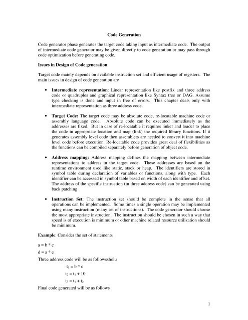
Example: Consider the set of statements
a = b * c
d = a * e
Three address code will be as followssholu
t1 = b * c
t2 = t1 + 10
t3 = t1 + t2
Final code generated will be as follows
1

MOV b, R0 / load b to register Ro,
MUL C, R0
MOV.R0, a Mov a to Ro and moving Ro to a can be eliminated
MOV a, R0
MUL e, R0
MOV R0, d
Redundant instruction should be eliminated.
Replace n instruction by single instruction
x = x + 1
MOV x, R0
ADD 1, R0 ⇒ INC x
MOV R0. x
Register allocation: If the operands are in register the execution is faster hence the set of
variables whose values are required at a point in the program are to be retained in the
registers.
Familiarities with the target machine and its instruction set are a pre-requisite for designing a
good code generator.
Target Machine: Consider a hypothetical byte addressable machine as target machine. It
has n general purpose register R1, R2 ------- Rn. The machine instructions are two address
instructions of the form
op-code source address destination address
Example:
MOV R0, R1
ADD R1, R2
Target Machine supports for the following addressing modes
a. Absolute addressing mode
Example: MOV R0, M where M is the address of memory location of one of the
operands. MOV R0, M moves the contents of register R0 to memory location M.
b. Register addressing mode where both the operands are in register.
Example: ADD R0, R1
c. Immediate addressing mode – The operand value appears in the instruction.
Example: ADD # 1, R0
2

d. Index addressing mode- this is of the form C(R) where the address of operand is at the
location C +Contents(R)
Example: MOV 4(R0), M the operand is located at address = contents
(4+contents(R0))
Cost of instruction is defined as cost of execution plus the number of memory access.
Example:
MOV R0, R1, the cost = 1 as there are no memory access.
Where as MOV R0, M cost = 2.
Register and address descriptor
Register descriptor gives the details of which values are stored in which registers and the list
of registers which are free.
Address descriptor gives the location of the current value can be in register, memory location
or stack based on runtime environment.
Code generation algorithm
Consider the simple three address code for which the target code to be generated.
Example: a = b op c
i.Consult the address descriptor for ‘b’ to find out whether b is in register or memory
location. If b is in memory location, generate code.
a. MOV b, Ri where Ri is one of the free register as per register descriptors.
Update address descriptor of b and register descriptor for free registers.
ii.Generate code for OP C, where C can be in memory location or in register.
iii.Store result ‘a’ in location L. L can be memory location M or register R, based on
availability of free register and further usage of ‘a’. Update register descriptor and
address descriptor for ‘a’ accordingly.
Example: x = y + z
Check for location of y,
Case 1: If y is in register R0 and z may be in register or memory. The instructions will be
ADD z, R0
MOV R0, x
In this case the result x has to be stored in memory location x.
Case2: If y is in memory, fetch y to register, update address and register descriptor
3

MOV y, R0
ADD z, R0
MOV R0, x
Example:
P = (x – y) + ( x – z) + ( x – z)
t1 = x – y
t2 = x – z
t3 = t1 + t2
t4 = t3 + t2
Three address code
3 addr M/c Code Cost Reg desc Addr desc
t1 = x – y MOV x , R0 2 R0 has t1 t1 in R0
SUB y , R0 = 2
t2 = x – z MOV x , R1 2 R0 has t1 T in R0
SUB z, 12 2 R1 has t2 U in R1
t3 = t1 + t2 ADD R1 , R0 1 R0 has t3
t4 = t3 + t2
ADD R1, R0
MOV R0, t4
1
2
R1 has t2
Example: Generate code for instruction x = y[i] and x [i]=y
t2 in R1
t3 in R0
R0 has t4 t4 in R0 and
memory
Stmt i in reg Ri i in Memory i in Stack
Code Cost Code Cost Code Cost
x = y [i] MOV y (Ri), R 2 MOV M, R 4 MOV Si (x), R 4
MOV b (R1, R2) MOV y (R), R
x [i] = y MOV y, x (Ri) 3 MOV M, R 5 MOV Si(x),x
MOV y, x (R)
5
Code generation for function call
Code generation for function code is base on the runtime storage. The runtime storage can by
static allocation or stack allocation. In case of static allocation the position of activation
record in memory is fixed at the compile time. To recollect about activation record,
whenever a function is called, activation records are generated, these records store the
parameters to be passed to functions, local data, temporaries, results & some machine status
information along with the return address. In case of stack allocation, every time a function
is called, the new activation record in generated & is pushed onto stack, once the function
completes, the activation record is popped from stack. The three address code for function
call consists of following statements
4

1. Call.
2. Return
3. end
4. action
Call statement is used for function Call, it has to mail the control to the function along with
saving the status of current function.
Return statement is used to give the control back to called function. Action defines other
operations or instructions for assignment or flow control statements. End indicates the
completion of operations of called function.
Static allocation: This section describes the final code generation for function calls, where
static allocation is used as runtime environment.
• Call statement : The code generated for call stmt is as follows.
MOV # current + 20, function.static_area
GOTO function.code_area
# current + 20 indicates the address of next instruction to which the return of function, i.e, the
instruction of called function which has to be executed after the called function completes
execution. 20 defines the size of goto statement following call stmt.
Function.static_area defines the address of activation record of function. Function.code_area
defines the address of 1 st instruction of called function.
• Return Statement: Code generated for return stmt is
goto * function.static_area.
This allows the control back to the called function.
Example:
/* code for main */
action 1
call fun
action 2
end
/* code for fun */
action 3
5

eturn
Three address code that will be generated for the above set of statements is as follows.
10: action 1
20: MOV # 40, 200 /* Save return address 40 at location 200 */
30: GOTO 100
40: Action 2
50: end
/* code for function */
100: action 3
100: GOTO * 200
200: 40(return address)
Stack allocation: Whenever the function is called the activation record of called fun c is
stored on Stack, once the function returns, it is removed from Stack. Final code that will be
generated for stack area for initialize the Stack is
MOV # Stack.begin, SP /* initialize the Stack Pointer */
SP denotes Stack Pointer.
Code for Call statement is as follows
Add # main.record size, SP /*main.recordsize referes to
record size of caller function*/
MOV # current +16, *SP /*Save return address*/
GOTO function.code_area
Return statement has the following target code.
GOTO *0(SP)
SUB # main.recordsize, SP
Example: For the below three address code
/* code for a */
action1
call c
action 2
end
6

* code for b */
action 3
return
/* code for c */
action 4
call b
action 5
call c
action 6
call c
return
The final code generated will be as follows:
/* code for a * /
100: MOV # 600, SP // initialize stack
110: action 1
120: ADD # a.size, SP
130: MOV # 150, * SP
140: GOTO 300
150: SUB # a_size, SP
160: action 2
170: end
/* code for b */
200: action 3
210: GOTO * 0(SP)
/* code for c */
300: action 4
310: ADD # c_size, SP
7

320: MOV #340, *SP
330: GOTO 200
340: SUB # c_size, SP
350: action 5
360: ADD # C_Size_SP
370: MOV # 390, * SP
380: GOTO 300
390: SUB # C_Size_SP
400: Action 6
410: ADD # C_Size_SP
420: MOV # 440, * SP
430: GOTO 300
440: SUB # C_Size_SP
450: GOTO *0(SP)
600: Stack Starts here
Code Optimization
Code Optimization phase in mainly use to optimize the code for better utilization of memory and
reduce the time taken for execution. Code optimization takes input from intermediate code generator
and performs machine independent optimization. Code optimizer may also take input from code
generator and perform machine dependent code optimization. Compilers that use code optimization
transformations are called as optimizing compilers. Code optimization does not consider target
machine properties for optimization (like register allocation and memory management) if input is
from intermediate code generator.
Code optimization tries to optimize that part of the code which are executed more number of times,
like statements within flow control block of for statement and while statement. This is because the
most programs always spend maximum execution time on executing only few statements Code
optimization analysis programs in two levels control flow analysis and data flow analysis. In control
flow analysis code optimization concentrates more on improving the code of inner loops than outer
statements, as inner loops are executed more number of times than outer ones. A detailed data flow
analysis is required for debugging the optimized code. Data flow analysis collects the information of
statistics about statements being executed more number of times. This information is used in the
process if optimization. Code optimization should be such that best results crop up with minimum
effort.
8

Code Optimization has to mainly achieve two goals
1. Preserve the meaning of code – The output generated before (without) Code Optimization
should be same as the code after optimization.
2. Optimization should reduce the cost of execution considerably. The effort spent on code
optimization should be worth it.
It implies that amount of time taken for optimization should be very less when compared to the
reduction of overall execution time. Generally, a fast non optimizing compilers are preferred for
debugging programs
Code improvement always need not be in code optimization phase. It can be incorporated in source
program or in intermediate code or on target code. In source program say, for sorting program, user
can choose different algorithm based on the cost function like minimum space or minimum time.
Each algorithm can be efficient it its own way or other, like quick sort is very fast on unsorted/random
array where as other sorting like bubble sort is efficient on partially sorted array. Intermediate code
can be improved by improving loops and efficient address calculation may give better results. In final
code generation phase, optimized code can be efficiently generated by selecting appropriate
instruction, use registers efficiently and some instruction transformations. Example: Keeping most
used variables in registers which avoids frequent fetching and storing in memory location. This
chapter deals with optimization of intermediate code represented as three address code. Intermediate
code is relatively independent at target machine so optimization is machine independent.
Programs are represented as flow graphs to study control flow and temporary variables are used to
store intermediate results help in data flow analysis. It is seen that compilation speed is proportional to
the size at program being compiled hence amount of time taken for code optimization should be
relatively less.
Principal of code optimizations
This sections deals with identifying that part of the program where optimization is required. By using
the concept of proper register allocation, elimination of dead code and finding the cost of instruction,
it is possible to improve the efficiency of program statements.
Unnecessary Operation
In a program there may be some part of code which never executes. It would be waste to generate
code for these statements. It may also happen that some of the values of temporary variables may
never be used. These are called as dead codes, it has to be removed. There can be some subexpression
whose value is computed many times. This can be optimized by calculating the value of
sub-expression only once and other statements can just use this value.
Example:
x = 1
while (x != 1)
{ …}
Statements of while never executed hence do not generate code for statements within while statement.
Example:
9

x = y + z
a = x + 10
p = y + z
b = p + 20
Both x and p computes same sub-expression hence generate code for x only once and p uses value of
x instead of re-computing from x & y.
After intermediate code generation it may so happen that there can be a jump statement whose target
statement is next statement itself. In this case jump statement should be avoided, which reduces code
generating time.
Constant Folding : If the assignment statement consists of only constants to the right hand side of
assignment statement. Then the value of the expression can be pre-computed.
Example: y = 2 * 5 + 6
The value of y can be computed as 16 and stored. Then the three address code generated would by
y=16 instead of
t1 = 2 * 5
t2 = t1 + 6
y = t2
This helps in constant propagation i.e, from the above example if y is used in any other expression,
instead of substituting y = 2 * 5+6 it can be substituted with y = 16.
Example:
y = 2 * 5 + 16
x = y + z
without optimization
x = 2 * 5 + 6 + z
with optimization
y = 16
x = 16 + z
Some of the operations like procedure call are very expensive, especially recursive procedure calls. In
order to reduce this, recursive procedures may be converted to iterative by providing lables. Issues
regarding procedure call it that before transferring the control to procedure. The status of procedure
has to be stored in registers. It has to be restored after procedure returns. Hence increases load and
store instructions.
Predicting program behavior
10

In order to generate more optimized code, Code optimization phase has to find out number of
variables used, their value set, those expressions which are used many times. It should also perform
some statistical analysis like-part of the code never reached, part of code which will executed many
times, procedures likely to be called. This information helps in adjusting loop structure and procedure
code to minimize execution speed.
Other Methods of Optimizations
Some of the optimization techniques are used to improve the loop statements. These are code motion
and reduction in strength of expression.
Code Motion:
Optimization is done for those statements which are executed frequently. Hence the statements whose
values do not change with respect to loop invariants should be removed from the loop.
Example:
a = 1;
while (a! = 10)
{
}
b = x + 100;
a = a + 1 ;
printf(“%d”,a);
In the above example, variable b with in while loop, is independent of loop invariant a and the value
of x do not change inside loop, hence b = x + 100 can be executed before while loop or after while
loop.
b = x + 100;
a = 1;
while (a ! = 0 )
{ a = a + 1;
}
printf (“%d”,a);
Reduce the strength of expression: If the intermediate code consists of multiplication or division, it
can be replaced by addition or subtraction, this reduces the strength of expression.
Example:
while ( i > 10)
{ i = i + 1;
11

}
t1 = 4 * i;
The statement with in while loop, will be executed until ‘i’ greater than 10. Initially if i = 0, for the
first iteration i = 1 and t1 = 4, for the 2 nd instruction i = 2 and t1 = 4 * 2 = 8
or t1 = 4 * (i + 1)
t1 = 4 * i + 4 (∴ t1 = 4 * i )
t1 = t1 + 4
As the expression for evaluating t1 which requires multiplication is reduced to addition, its execution
is faster.
Local, Global & Inter-Procedural Optimization:
In case of local optimization straight line codes with in basic block are optimized. The basic block
consists of only assignment statements with no jumps or loops. Some of the optimization techniques
that can be used for local optimization are constant folding, constant propagations and algebraic
transformations.
Optimization considering many basic blocks of single procedure is called global optimization. They
use optimization techniques like code motion, elimination of induction variables and reduction in
strength of expression. Global optimization requires data flow analysis to detect jump boundaries
before optimization.
Inter-procedural optimization deals with optimization of entire program as a whole. This is very
difficult to achieve as it has to take care of different parameters passing mechanization and non local
variable access. The advantage of inter procedural optimization is that each procedure can be
optimized independently and linked together at the end with the help of linker which performs
optimization later on.
Machine dependent optimization
Some of the optimizations are machine independent, like register allocation and cost of instruction.
Register Allocation:
Number of times variable in each block of program may vary, but there are fixed number at register in
the system. Hence these registers are to be efficiently used. As far as possible the temporary variable
or intermediate values should be present in register this reduces the load and store to memory.
Example:
x = y + z
a = x + 10
b = x + 20
As the value of x is used after it has been assigned a value. Retain the value of x in the register, to
avoid storing and reloading from memory.
Cost of Instructions:
12

Each instruction takes some machine cycles to perform the operation. The optimization strategies
should be such that it should reduce the number of machine cycles or in other words the strength of
instruction should be reduced to have better optimization.
Example:
x 2 can be replaced by expression x * x.
Expressions like adding 0 or multiplying by 1 can be removed, as these do not change the value of
variable.
Example:
1) x = x + 0
2) a = a * 1
These instructions can be eliminated as they do not change the value of x and a.
This is called algebraic transformation.
Data Structure:
Syntax trees can be used for some of the optimization techniques like constant folding, constant
propagation etc., but for optimization like eliminating loop invariant, or dead code elimination, it is
not very efficient, Specially for global optimization syntax tree is not efficient as it requires the study
for control flow. Hence flow graphs are used. Flow graphs consist of basic blocks as nodes and edges
connecting basic blocks indicate the control flow. The sequence of three address statement is
converted to flow graph using following steps.
1. Construct basic block
2. Generate flow graph
1. Construction of Basic Blocks
a) Determine set of header statements. Header statements are the first statement of each basic
block.
b) First statement is a header statement
c) Any statement which is target of conditional or unconditional jump is a header statement.
d) Any statement following conditional or unconditional jump is a header statement.
2. Construct flow graph
Construct graph with B1 as the stating node where B1 is basic block which has first statement of the
program. Generate edge from Bi to Bj if control flows from block Bi to Bj. Entry for any block Bk
will be from the first statement of Bk and exit from Bk will be from last statement only. No
intermediate jump or return can happen in the basic block.
Example: Consider the following C statement
for i = 1 to n do
13

for i =1 to n do
C[i, j] = 0;
Three address code generated will be as follows
1) i = 0
2) if i < n go to 4
3) go to 15
4) j = 1
5) if j < n go to 7
6) go to 13
7) t1 = i * 10
8) t2 = t1 + j
9) t3 = 4 * t2
10) C[t3] = 0
11) j = j + 1
12) go to 5
13) i = i + 1
14) go to 2
15)
Basic blocks will be as follows
Stmt no Header Three address code Block no
1 H i = 0 B1
2 H if i < n go to 4 B2
3 H go to 15 B3
4 H j = 1 B4
5 H if j < n go to 7 B5
14

6 H go to 13 B6
7
8
9
10
11
12
13
14
15
H t1 = i * 10
t2 = t1 + j
t3 = 4 * t2
C[t3] = 0
j = j + 1
go to 5
H i = i + 1
go to L6
Flow graph for the basic blocks is as follows in Fig 9.1
B6
B8
Directed Acyclic Graph
B4
B5
B7
B1
B2
B3
B7
B8
Fig 9.1 Flow graph for the basic blocks
15

Flow graphs are mainly used for global optimization. These are not very efficient for local
optimizations on basic blocks. Hence Directed A cyclic Graphs (DAG) is used. Leaves of DAG are
used to represent variable names or constants. Interiors nodes and root of DAG is used to represent
operator symbol. Nodes have label which denotes the most recent value for the variables.
For any statement a = b op C the DAG is in Fig 9.2
b c
Fig 9.2 DAG for the expression a = b op c
b,c the leaves represents variables. Interior node OP represents operator OP and a is the label for OP
which gives the value of b OP c.
For exp like x = y no node is created for x. Only the label y will be added to the node which had label
x.
Example: Consider the following code
t1 = a + b
t2 = t1
Fig 9.3 DAG for the three address code
DAG for the three address code is represented in Fig 9.3. For 2 nd expression no new node is created,
but it will use the same node +. Initially t1 will be the label of + after 2 nd statement t2 is also added as
label of ⊕
Example: Consider the following statements
a = b + c
b = a – d
t2, t1
*
a b
a
OP
b1
Ө
a0 ⊕ d0
b0 c0
16

Fig 9.4 DAG for the three address code
Fig 9.4 shows the DAG for the above three address code
Example: Consider the following statements
c = c + d
e = b + c
Fig 9.5 shows the DAG for the above three address code
Fig 9.5 DAG for the three address code
Example: Consider the following expression
a = -b * c + d
The three address code will be
t1 = –b
t2 = t1 * c
t3 = t2 + d
a = t3
b
⊕ e
c1 ⊕ b
c0 d0
a, t3 ⊕
t2 * d
t1Ө c
17

Fig 9.6 DAG for the three address code
Fig 9.6 shows the DAG for the expression a = -b * c + d represented as three address code
Example: Consider the following expression
a = b * d + b * d + c
The three address code will be
t1 = b * d
b2 = b * d
t3 = t1 + t2
t4 = t3 + c
a = t4
Fig 9.7 DAG for the three address code
Fig 9.7 shows the DAG for the expression a = b * d + b * d + c represented as three address code.
From the above DAG it is found that node * has 2 labels t1 & t2. Hence there is no necessary to
generate code twice for the same expression. Final code can be generated from DAG by topological
sorting. Topological sorting is the traversal of tree from leaf to root in which children are visited
before their parents. As there can be multiple topological sorts. There can be many code sequences for
single DAG.
Example:
Consider intermediate code
t1 = a + b
a = t1
t2 = b – 1
b = t2
t3 = b + 5
t1, t2 *
b d
t4 , a ⊕
t3 ⊕ c
⊕ t3
a1 t2 ⊕ Ө t2 , b1 5
a0 b 1
18

After topological sorting
t2 = b – 1
t1 = a + b
a = t1
t3 = b + 5
b = t2
Fig 9.8 DAG for the intermediate code
Reordering of code helps in eliminating unnecessary use of temporaries. Hence the code would be as
follows.
a = a + b
b = b – 1
t3 = b + 5
DAG gives the information of how many references exists for node. This helps in good register
allocation. If a value has many references then it can be retained in registers for long time. If the
value has no reference it can be removed from the register.
19