Quanto Adjustments in the Presence of Stochastic Volatility

More documents

Recommendations

Info

underlying S at time T converted with a fixed FX rate of one into to the currency Y. Thus, the quanto forward is given as the expected value of S(T ) under the measure Q Y : F q (t, T ) = E QY [S(T )] = S(t)e (rX −d)(T −t) × E QY � e −ρS,F � T � 1 T X σF X ν(s)ds− t 2 t ν(s)2 � T ds+ρS,ν t = S(t)e (rX −d)(T −t) E Q Y QY ν(s)dWν (s)+ √ 1−ρ2 � � T S,ν ν(s)dW (s) t � e −ρS,F � T 1 X σF X ν(s)ds− t 2 ρ2 � T S,ν t ν(s)2 � T ds+ρS,ν t where we expressed the Brownian motion W QY S as W QY S (t) = ρS,νW QY � ν (t) + 1 − ρ2 S,νW (t) � QY ν(s)dWν (s) with W being a QY-Brownian motion independent of W QY ν and used the tower property. According to (4) and Itô’s Lemma we have dν(t) 2 � 2 δ = 2κ 2κ + ˆ θν(t) − ν(t) 2 � dt + 2δν(t)dW QY ν (t) and � T t ν(s)dW QY ν (s) = 1 � ν(T ) 2δ 2 − ν(t) 2 − δ 2 (T − t) − 2κˆ � T � T θ ν(s)ds + 2κ ν(s) t t 2 � ds . (5) Using the last equation we obtain for the quanto forward: F q (t, T ) = S(t)e (rX −d)(T −t)− ρS,ν 2δ (ν(t) 2 +δ 2 � Y (T −t)) Q E e −s1 � T t ν(s)2 � T ds−s2 ν(s)ds+s3ν(T )2� t and applying Lemma 1 of the appendix finally yields with F q (t, T ) = S(t)e (rX −d)(T −t)− ρ S,ν 2δ (ν(t) 2 +δ 2 (T −t)) D (t, T, ν(t), s1, s2, s3) (6) s1 = − 1 � 2κρS,ν 2 δ − ρ2 � S,ν , s2 = κˆ θρS,ν δ + ρS,F XσF X, s3 = ρS,ν 2δ . The function D is given in Lemma 1. Since quanto forwards are often liquidly traded, the closed-form solution (6) allows us to calibrate the model quickly to market quotes for quanto forwards. 3 Quanto options The purpose of this section is to derive closed-form solutions for standard quanto options within the model framework described in the previous section. Let C q (t, T, K) denote the price of a quanto call option with strike K and maturity T. Then we have C q (t, T, K) = e −rY � Y (T −t) Q E (S(T ) − K) +� with Q Y 1 defined by the Radon-Nikodym derivative Thus, the quanto call option price can be written as = e −rY (T −t) F q (t, T )Q Y 1 [S(T ) > K] − e −rY (T −t) KQ Y [S(T ) > K] dQY 1 S(T ) = dQY F q (t, T ) . C q (t, T, K) = e −rY (T −t) F q (t, T )P1 − e −rY (T −t) KP2 4 (7)
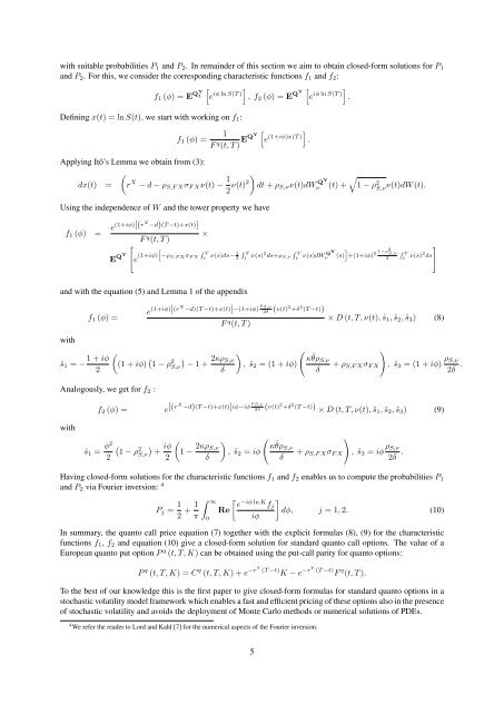
with suitable probabilities P1 and P2. In remainder of this section we aim to obtain closed-form solutions for P1 and P2. For this, we consider the corresponding characteristic functions f1 and f2: f1 (φ) = E QY � � 1 iφ ln S(T e )� QY iφ ln S(T , f2 (φ) = E e )� . Defining x(t) = ln S(t), we start with working on f1: f1 (φ) = 1 F q � (1+iφ)x(T EQY e )� . (t, T ) Applying Itô’s Lemma we obtain from (3): dx(t) = � r X − d − ρS,F XσF Xν(t) − 1 2 ν(t)2 � dt + ρS,νν(t)dW QY � ν (t) + 1 − ρ2 S,νν(t)dW (t). Using the independence of W and the tower property we have f1 (φ) = e(1+iφ)[(rX −d)(T −t)+x(t)] E QY � F q (t, T ) e (1+iφ) � −ρS,F X σF X and with the equation (5) and Lemma 1 of the appendix f1 (φ) = × � T t � 1 T ν(s)ds− 2 t ν(s)2 � T ds+ρS,ν t e (1+iφ)[(rX −d)(T −t)+x(t)]−(1+iφ) ρ S,ν 2δ (ν(t) 2 +δ 2 (T −t)) F q (t, T ) � QY ν(s)dWν (s) +(1+iφ) 2 1−ρ2 S,ν � T 2 t ν(s)2 � ds × D (t, T, ν(t), ˆs1, ˆs2, ˆs3) (8) with � 1 + iφ ˆs1 = − (1 + iφ) 2 � 1 − ρ 2 � � � 2κρS,ν κ S,ν − 1 + , ˆs2 = (1 + iφ) δ ˆ θρS,ν δ + ρS,F � XσF X , ˆs3 = (1 + iφ) ρS,ν 2δ . Analogously, we get for f2 : with f2 (φ) = e [(rX −d)(T −t)+x(t)]iφ−iφ ρ S,ν 2δ (ν(t) 2 +δ 2 (T −t)) × D (t, T, ν(t), ˜s1, ˜s2, ˜s3) (9) ˜s1 = φ2 2 � � � 2 iφ 1 − ρS,ν + 1 − 2 2κρS,ν � � κ , ˜s2 = iφ δ ˆ θρS,ν δ + ρS,F � XσF X , ˜s3 = iφ ρS,ν 2δ . Having closed-form solutions for the characteristic functions f1 and f2 enables us to compute the probabilities P1 and P2 via Fourier inversion: 4 Pj = 1 1 + 2 π � ∞ Re 0 � e −iφ ln K fj iφ � dφ, j = 1, 2. (10) In summary, the quanto call price equation (7) together with the explicit formulas (8), (9) for the characteristic functions f1, f2 and equation (10) give a closed-form solution for standard quanto call options. The value of a European quanto put option P q (t, T, K) can be obtained using the put-call parity for quanto options: P q (t, T, K) = C q (t, T, K) + e −rY (T −t) K − e −r Y (T −t) F q (t, T ). To the best of our knowledge this is the first paper to give closed-form formulas for standard quanto options in a stochastic volatility model framework which enables a fast and efficient pricing of these options also in the presence of stochastic volatility and avoids the deployment of Monte Carlo methods or numerical solutions of PDEs. 4 We refer the reader to Lord and Kahl [7] for the numerical aspects of the Fourier inversion. 5
Page 1 and 2: Quanto Adjustments in the Presence
Page 3: Furthermore, we assume an investor
Page 7 and 8: Table 1: Model Parameters ν0 κ θ
Page 9 and 10: Table 3: Model Parameters for Doubl
Page 11: A Appendix Lemma 1. Let ν be a mea

Quanto Adjustments in the Presence of Stochastic Volatility

You also want an ePaper? Increase the reach of your titles

Delete template?

Save as template?