Multidimensional data modeling for location-based services

The VLDB Journal (2004) 13: 1–21 / Digital Object Identifier (DOI) 10.1007/s00778-003-0091-3
Multidimensional data modeling for location-based services
Christian S. Jensen, Augustas Kligys, Torben Bach Pedersen, Igor Timko
Aalborg University, Department of Computer Science, Fredrik Bajers Vej 7E, 9220 Aalborg Øst, Denmark;
e-mail: {csj,augustas,tbp,timko}@cs.auc.dk
Edited by J. Veijalainen. Received: 28 September 2002 / Accepted: 5 April 2003
Published online: August 12, 2003 – c○ Springer-Verlag 2003
Abstract. With the recent and continuing advances in areas
such as wireless communications and positioning technologies,
mobile, location-based services are becoming possible.
Such services deliver location-dependent content to their
users. More specifically, these services may capture the movements
and requests of their users in multidimensional databases,
i.e., data warehouses, and content delivery may be based
on the results of complex queries on these data warehouses.
Such queries aggregate detailed data in order to find useful
patterns, e.g., in the interaction of a particular user with the
services.
The application of multidimensional technology in this
context poses a range of new challenges. The specific challenge
addressed here concerns the provision of an appropriate
multidimensional data model. In particular, the paper extends
an existing multidimensional data model and algebraic query
language to accommodate spatial values that exhibit partial
containment relationships instead of the total containment relationships
normally assumed in multidimensional data models.
Partial containment introduces imprecision in aggregation
paths. The paper proposes a method for evaluating the imprecision
of such paths. The paper also offers transformations of
dimension hierarchies with partial containment relationships
to simple hierarchies, to which existing precomputation techniques
are applicable.
Keywords: Location-based services – Multidimensional data
– Data modeling – Partial containment
1 Introduction
Several trends in hardware technologies combine to enable the
deployment of mobile, location-based e-services. These trends
include continued advances in the miniaturization of electronics
technologies, in display devices, and in wireless communications.
Other trends include the improved performance of
general computing technologies and the general improvement
in the performance/price ratio of electronics. Perhaps most importantly,
geopositioning is becoming increasingly available
and accurate.
Correspondence to: I. Timko
It is expected that the coming years will witness very
large quantities of wirelessly Internet-worked objects that are
location-enabled and capable of movement to varying degrees.
Examples of objects of interest here include consumers using
Internet-enabled mobile-phone terminals and personal digital
assistants, tourists carrying online and position-aware “cameras”
and “wrist watches,” vehicles with computing and navigation
equipment, etc.
These developments pave the way to a range of qualitatively
new types of Internet-based services [12]. These types
of services—which either make little sense or are of limited
interest in the traditional context of fixed-location, desktop
computing—include the following: traffic coordination, management,
and way-finding, location-aware advertising, integrated
information services, e.g., tourist services, safety-related
services, and location-based games that merge virtual
and physical spaces.
A single generic scenario may be envisioned for these
location-based services. Moving service users disclose their
positional information to services, which in turn use this and
other information to provide specific content and functionality.
The services capture the requests they receive, including their
geographical origins, in a multidimensional database, i.e., a
data warehouse. We note that the privacy of service users is
a concern and that legislation is available that regulates this
aspect (e.g., [8]). We are aware that some service providers
require each customer to enter into an explicit agreement with
the provider that covers the provider’s possible use of the customer’s
location data.
Querying the resulting data warehouse enables the services
to analyze their interactions with the users, thus allowing
the services to customize their interactions with the users. As
a result, each user receives a service customized to the user’s
specific preferences and needs and current situation. For example,
the query “show the number of requests per district for
user X” provides valuable information about the geographical
behavior of user X. In addition, the accumulated data are
used by the service providers for delayed modification of the
services provided and for longer-term strategic decision making.
For example, the query “show the number of requests per

2 C.S. Jensen et al.: Multidimensional data modeling for location-based services
city per quarter for the last year" gives information about the
changes in service use for different cities over time.
A data warehouse [1,15,25] is a large repository that organizes
data specifically for analytical purposes by employing
a multidimensional view of data. Multidimensional models
view a central data element for the given domain, e.g., a service
request, as a fact (also termed a cell), which is uniquely
defined by a combination of dimension values, each of which
stems from one of a number of hierarchically organized dimensions.
Typical dimensions are the location from which the
request originates, the profile of the user that has issued the
request, and the time of the request. Dimensions are organized
as hierarchies of levels, also termed categories. For example,
the time dimension may have Day, Week, Month, Quarter, and
Year levels.
The multidimensional view is particularly well suited for
complex data analyses, which include data aggregation [25],
i.e., the counting of facts that are characterized by specific
values from the dimensions. Typical operations on multidimensional
data warehouses use the dimension hierarchies to
dynamically change the level of detail in order to gain an understanding
of a particular phenomenon.
If more detail is desired, e.g., to understand why the number
of requests dropped sharply in Q4 2002, a “drill down” is
performed, where numbers of requests per month are used in
place of numbers of requests per quarter. If the opposite is true,
i.e., less detail is desired in order to get a better overview, a
“roll up” is performed. This means that it is crucial for multidimensional
data warehouses to have well-designed dimension
hierarchies that capture the useful levels of detail. We assume
this kind of data analysis in our scenario.
The scenario is realistic. For example, the Danish company
Euman A/S [7] has developed and deployed a service
delivery system capable of providing location-based services.
Although the current object-relational database underlying
the system is not optimized for complex data analyses, the
database contains data, e.g., data on geo-referenced transportation
infrastructure, that can be used to implement a multidimensional
data warehouse. This in turn enables complex multidimensional
analyses of the interactions among the services
delivered by the system and the users.
The scenario entails the capture of spatial data in a multidimensional
data warehouse. This poses new challenges. For
example, an appropriate data model should support irregular,
so-called nonnormalized, dimension hierarchies [26] where
the hierarchies are not balanced trees. Next, while dimension
values in conventional multidimensional data models either
are disjoint or exhibit total containment relationships, partial
containment is prevalent in spatial data. For example, a roadway
that extends from a city into a rural area is only partially
contained in the city. Thus, partial containments between dimension
values, i.e., location values such as roadways and
cities, must be supported by the data model. The inclusion
of advanced modeling facilities in a data model should not
preclude the provision of an efficient implementation of the
data model. In a multidimensional context, this implies that
conventional preaggregation techniques [32] should remain
applicable.
This paper first analyzes the mobile e-service application
domain, formulating requirements to a data model. It then
presents a new multidimensional data model with an accompanying
algebraic query language that arguably meets the requirements.
Notably, the model supports nonnormalized hierarchies
and partial containment. Partial containment, together
with its transitivity property, is the key new aspect of the
model, and the paper treats this topic in detail.
Partial containment introduces additional imprecision in
aggregation paths. Because it is important to be able to evaluate
the imprecision of a path (e.g., for choosing the most
precise one), the paper offers a path imprecision evaluation
method. Practical preaggregation, i.e., precomputation of select
aggregate results that can be reused to obtain other aggregates,
is a technique that is essential for efficiently implementing
any multidimensional data model, including the
one proposed here. We thus propose algorithms for making its
dimension hierarchies onto, covering, and aggregation strict.
This enables the application of standard preaggregation techniques
in an implementation of the model.
This paper is a revised and substantially extended version
of an earlier conference paper [13]. In particular, the contents
of Sects. 4.7, 5, 6, 7, and the appendix are entirely new.
The remainder of the paper is structured as follows. Section
2 discusses related work. Section 3 describes key requirements
of a multidimensional data model for location-based
services, and Sect. 4 then presents a data model that aims to
satisfy those requirements. Section 5 completes the description
of the model by defining its algebraic query language.
Section 6 presents the method for evaluating the imprecision
of an aggregation path. Section 7 provides an overview of the
algorithms for normalizing dimension hierarchies. Section 8
concludes and points to future work. The appendix provides
the details of the normalization algorithms. The paper can be
read and understood without reading the appendix.
2 Related work
In the domain of spatial data modeling, most related scientific
and industrial work is dedicated to object-relational extensions
of SQL. In particular, Egenhofer [6] proposed a spatial
model and query language that compared favorably to several
related languages. A spatiotemporal model and a query language
were formally defined by Güting et al. [10]. Dedicated
designs of spatial relational algebras with formal semantics
were also proposed by Scholl and Voisard [31] and Gorgano
et al. [2]. As for industrial standards, the Open GIS Consortium
[20] adopted a specification [19] for implementation of
a spatial SQL extension, and Oracle Spatial [17] conforms to
this specification.
In essence, these works develop means of analyzing spatial
data, given, among other things, varying relationships between
spatial objects, e.g., overlapping, containment, etc. However,
we believe that the object-relational view of data does not
fully support complex data aggregation. In part, this is due to
the lack of hierarchies. We therefore develop a multidimensional
data model and algebra that are capable of capturing
an advanced kind of relationship between spatial objects, i.e.,
partial containment relationships.
Multidimensional data warehouses [1,15,25] are generally
accepted as the most powerful platform for data analysis in
terms of expressive power and performance. Expressive power
is achieved mainly by using the multidimensional concepts of

C.S. Jensen et al.: Multidimensional data modeling for location-based services 3
dimensions and hierarchies. Good performance is achieved
primarily by using preaggregation, i.e., storing precomputed
results of aggregate queries and using these to answer new
queries more efficiently. However, current multidimensional
database technology does not support the complex structures
needed to handle complex spatial information.
To the authors’ knowledge, no other existing multidimensional
data model offers built-in support for partial containment
hierarchies. This deficiency is also suggested by surveys
of multidimensional data models [26, 33]. However, rather
than proposing an entirely new multidimensional data model
and query language, the proposed model and query language
extend a previously proposed multidimensional model and algebra
[23,26]. The model that we extend was chosen because
it is formally defined and because it compares favorably to
14 related data models [26]. The paper’s algorithms for the
normalization of partial containment dimension hierarchies
extend algorithms presented by Pedersen et al. [22,24] for use
with the model being extended.
Pedersen and Tryfona [27] propose a slightly different approach
to the multidimensional modeling of spatial data. They
ignore partial containment relationships among hierarchy values
and instead consider spatial facts, i.e., values characterized
by hierarchy values, that are two-dimensional regions.
Their focus is on how to support practical preaggregation with
such overlapping facts. The conceptual model underlying their
work is the model being extended here.
Ferri et al. [9] propose a method to couple a multidimensional
data model with a Geographical Information System
(GIS) to combine the strengths of these technologies. Modern
GISs such as ArcInfo [14] and MapInfo [3] provide some
support for complex geostatistical and spatial analysis. Currently,
the systems neither directly support multidimensional
data modeling nor use preaggregation. Incorporation of these
features into the systems would enable complex data aggregation
queries and consequently enhance analytical capabilities
of the systems. As a result, it would be possible to use the systems
in our scenario of customizing location-based services
to users’ needs.
The area of “imperfect” data has received a great deal of attention
in general as well as specialized database contexts [5].
Within multidimensional databases, work has been done on irregular
multidimensional data [4,15,26,29] and the associated
summarizability problems [16,26,28]. However, none of these
works consider partial containment dimension hierarchies.
In the industrial domain, linear referencing [30] has been
used quite widely for the positioning of business data, e.g.,
user locations and other points of interest, located along linear
elements (e.g., roadways) in transportation infrastructures.
For example, Oracle Spatial [17] offers support for linear referencing.
In addition, a generic data model [18] has been recommended
for the capture of different aspects of entire transportation
infrastructures and related business data. By applying the
multidimensional view on linearly referenced data, we would
enable complex aggregation queries on this kind of business
data. In order to achieve this, it is necessary that a multidimensional
model provide support for nonnormalized partial
containment hierarchies. For this reason, we believe that our
model, which supports hierarchies of this type, could serve as
a basis for complex analysis of linearly referenced data.
Finally, the World Wide Web Consortium [35] has recently
published a draft specification [34] of an XML-based language
for describing location information. In our scenario, that language
could facilitate data exchange.
3 Usage scenario and requirements
We introduce a prototypical usage scenario for a multidimensional
database in the context of location-based services, and
we use this scenario to illustrate important requirements to a
multidimensional data model. The scenario is also used for
exemplification throughout the paper.
3.1 Usage scenario
In our prototypical usage scenario, a user issues a service request
that is characterized by a combination of values including
values that capture the time and date of the request, the
profile of the user, and the location from which the request
originates.
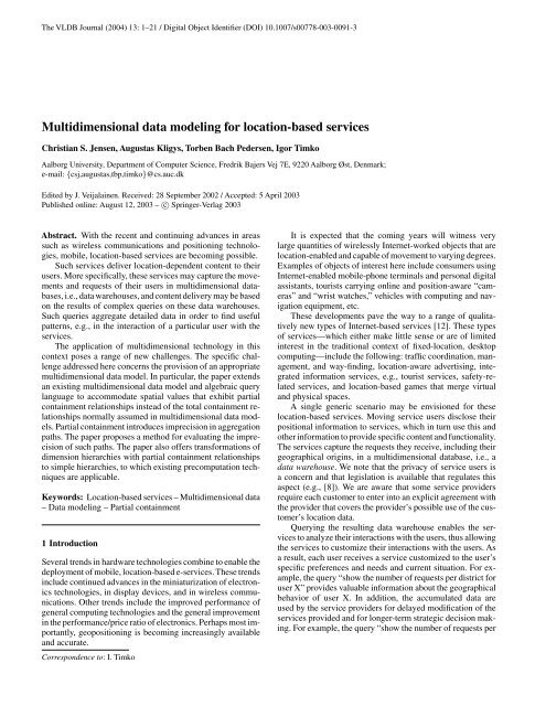
The ER diagram in Fig. 1 describes location values that
may be used for capturing the origins of service requests as
well as location values that may prove useful in analyses of
service requests that involve the origins of the requests. The
meanings of most of the entity types found in the diagram
follow from the names of the types, though there are some exceptions,
namely, the entity type IP Address represents fixed
IP addresses, e.g., those of office or home desktop computers,
the type Cell represents wireless network cells, the type District
represents city districts, and the type Roadway represents
all types of roads.
The schema is meant to illustrate certain problematic properties
of locations, such as partial containment hierarchies,
while still maintaining simplicity. The schema is not meant
to capture all aspects of locations. For example, generic international
locations or locations in oceans are not handled. For
information on how to model international locations, we refer
to the literature [15].
The diagram uses its naming convention to distinguish between
two different types of binary relationships between entities,
namely, full and partial containment relationships among
the spatial extents of the related entities. In the diagram, an
“F” in a relationship name indicates a total, or full, containment
relationship type, and a “P” indicates that only partial
containment may be assumed.
For example, consider the relationship type co-F-ro between
entity types Coordinate and Roadway, and consider ro-
P-di, which relates Roadway and District. The meaning is that
a coordinate is either fully contained or not contained in a roadway,
which, in turn, may be fully or (only) partially contained
in a district.
Note that all the relationship types in the diagram are stored
relationship types. For example, with the relationship types co-
F-ro and ro-P-di present in the diagram, the relationship type
co-F-di may seem redundant. However, this third relationship
type captures nonredundant information. For example, some
coordinates are not contained in any roadways, but are still
contained in districts.

4 C.S. Jensen et al.: Multidimensional data modeling for location-based services
All locations
(1,n)
co-F-al
IP address
(1,1)
Country
(1,n)
(0,1)
(0,1)
(1,n)
co-F-ip
ip-F-ci
ip-F-pr
pr-F-co
(0,n)
(1,n)
(1,n)
(1,1)
Province
(1,n)
(1,n)
(1,n)
ci-F-pr
di-F-pr
co-F-pr
(1,1)
(1,1)
(1,1)
City
(0,n)
(1,n)
ce-P-pr
(1,n)
(1,n)
(1,n)
di-P-ci
(1,n)
(1,n)
(0,n)
ce-P-ci
ro-P-co
(1,n)
ro-P-pr
(1,n)
ro-P-ci
(1,n)
(1,n)
District
(1,n)
co-F-ci
(0,1)
(0,n)
ro-P-di
Cell
(0,n)
(1,n)
(1,n)
co-F-ce
(0,1)
(0,n)
ce-P-di
(0,n)
Roadway
(1,n)
co-F-ro
(0,1)
Coordinate
co-F-di
(0,1)
Fig. 1. Location ER diagram
The existence of a partial containment relationship type
between two entity types in the case study also implies the existence
of a full containment relationship type between these
two entity types, as full containment is a special case of partial
containment. The intuition is that if objects of one type may
be partially contained in objects of another type, then some
objects of the former type may also be fully contained in objects
of the latter type, although fewer objects will satisfy this
relationship.
In a multidimensional schema, user requests will be modeled
as facts and the values that characterize the user requests
are organized into dimensions. For our scenario, we will have
three dimensions. The TIME dimension captures the time of
the user requests and has categories (levels) such as Second,
Minute, and Hour. The USER dimension captures aspects of
the users issuing the requests. It has categories such as Spoken
Language, Personal Interest, Actual Age, and Main Occupation.
The LOCATION dimension captures the (possibly
changing) locations of the users when the users issue requests.
Entity types in the Location ER diagram are then represented
as categories in the hierarchy of categories that makes up the
LOCATION dimension, and relationship types in the Location
ER diagram may be represented as relationships among
categories in the LOCATION dimension. It is normal practice
in multidimensional modeling to include only some of
the relationships found in the source data, the primary driver
being to obtain hierarchies useful for roll-up/drill-down operations
[15].
In Sect. 4, we illustrate how the Location ER diagram is
mapped to the LOCATION dimension. In particular, the issues
involved in deciding how the LOCATION dimension should
be modeled are discussed in detail in Sect. 4.7.
As noted above, the presented usage scenario is based on
a real-world location-based service delivery system [7]. The
database of this system contains the data necessary for implementing
a multidimensional data warehouse. For example, the
available data on geo-referenced transportation infrastructure
can be used to build a LOCATION dimension. Although the
available data do not directly capture containment relationships
between spatial entities, they can be inferred from the
data.
3.2 Data model requirements
Next we discuss the requirements for a multidimensional data
model that contends with our usage scenario. While the requirements
are all highly relevant to our context, most of them
are more general and were formulated earlier. We describe the
requirements only briefly and refer to the literature for further
detail [26]. Other requirements are given elsewhere [11].

C.S. Jensen et al.: Multidimensional data modeling for location-based services 5
1. Explicit and multiple hierarchies in dimensions Dimension
values are partitioned into categories of values, and
categories are related via containment relationships. For
example, coordinates belong to a Coordinate category, and
Coordinate is contained in Country, meaning that coordinates
are contained in countries. Explicit hierarchies are
highly useful in data analysis as they are used for aggregating
data to the right level of detail in exploratory analyses
that use roll-up/drill-down operations [25]. Support for
multiple hierarchies means that multiple aggregation paths
are possible. These are important for a number of reasons.
The key reason is that multiple hierarchies exist naturally
in much data. Another reason is that these enable better
handling of the imprecision in queries caused by partial
containment in dimension structures. For example, in the
LOCATION dimension, we obtain a more precise result if
roadways are rolled up to countries directly than if roadways
are rolled up to countries through districts, cities, and
provinces.
2. Partial containment We have seen that two spatial values
may be not only either disjoint or have one contained in the
other; they may overlap. A multidimensional data model
should provide built-in support for dimensions with partial
containment relationships. This will increase the modeling
power of the model and enable new kinds of queries.
Specifically, we will be able to perform aggregation of data
along hierarchies with partial containment (e.g., districts
would, though approximately, roll up to cities).
3. Nonnormalized hierarchies Situations occur naturally
where a hierarchy value has more than one parent, a value
has no relationship to any value in the category immediately
above it in the dimension hierarchy, or a value has
no relationship to any value in any category below it. For
example, a roadway value may be related to several district
parent values, and a city value may have no cell child
values.
4. Different levels of granularity In our scenario, user requests
are characterized by values drawn from the dimensions.
Support for different levels of granularity enables a
request to refer to other values than those in the category
at the lowest level of a dimension hierarchy. For example,
the position of the user may be known at the level of a
coordinate (precise) or at the level of a mobile phone cell
(imprecise).
5. Many-to-many relationships between facts and dimensions
This requirement implies that a fact may be related
to more than one value in a dimension. For example, this
is useful in a situation where a request is related to more
than one service user.
6. Handling of imprecision When facts are characterized
by dimension values from different levels, imprecision in
the data occurs. In addition, partial containment introduces
imprecision. Both types of imprecision may lead to imprecise
aggregate query results. In the first case, a result may
be imprecise because data for a query is missing. In the
second case, the transitive relationships between members
of aggregation paths may become imprecise (see Sect. 6
for details), rendering the results of queries imprecise. This
calls for means of handling imprecision.
We base our proposal for a new model on an existing data
model that satisfies Requirements 1, 3, 4, and 5. Moreover,
Requirement 6 is partially satisfied by the algebra associated
with the preexisting model. However, Requirement 2 (partial
containment) is not met by this or any other existing model.
4 Data model
This section extends the existing multidimensional data model
[26] to support partial containment. The section also presents
properties of the new model, considers its fulfillment of the
requirements, and discusses how to use it when designing dimensions.
4.1 Data model definition: dimension schemas
An n-dimensional fact schema is a two-tuple S =(F, D),
where F is a fact type and D = {T i ,i = 1,...,n} is a
set of dimension types. A dimension type T is a four-tuple
(C T , ⊏ T ,⊤ T , ⊥ T ), where C T = {C j ,j =1,...,k} are category
types of the dimension type T , and ⊏ T is a partial order
on the set C T . Next, ⊤ T is the top element of the order, meaning
that ∀C ∈ C T \{⊤ T } (C ⊏ T ⊤ T ). Symbol ⊥ T is the
bottom element; the precise meaning of this will be described
shortly. A function Anc : C T ↣ 2 C T
is defined that returns
the set of immediate ancestors of a category type C j . Function
Desc : C T ↣ 2 C T
returns the set of immediate descendants
of C j . The relation ⊏ T captures the full containment relationships
between category types.
We extend the definition of a dimension type by introducing
an additional relation ⊏ P T ⊆ C T ×C T . This new relation
captures the partial containment relationships between category
types. The properties of the new relation, which are
properties of a partial order, are as follows:
1. ∀C ∈ C T (C ̸⊏ P T C) (antireflexivity)
2. ∀(C i , C j ) ∈C T ×C T
((C i ⊏ P T C j) ⇒ (C j ̸⊏ P T C i)) (antisymmetry)
3. ∀(C i , C j , C k ) ∈C T ×C T ×C T
(((C i ⊏ P T C j) ∧ (C j ⊏ P T C k)) ⇒ (C i ⊏ P T C k)) (P-to-P
transitivity)
Relations ⊏ T and ⊏ P T are related as follows:
∀(C i , C j , C k ) ∈C T ×C T ×C T
1. ((C i ⊏ P T C j) ∧ (C j ⊏ T C k )) ⇒ (C i ⊏ P T C k)) (P-to-F
transitivity)
2. ((C i ⊏ T C j ) ∧ (C j ⊏ P T C k)) ⇒ (C i ⊏ P T C k)) (F-to-P
transitivity)
After the extension, a dimension type T is a five-tuple:
(C T , ⊏ T , ⊏ P T , ⊤ T , ⊥ T )
We use the notation ⊏ (P )
T
to indicate the union of the
two orders ⊏ T and ⊏ P T . With this notation in place we
can define the meaning of ⊥ T being the bottom element:
∀C ∈ C T \{⊥ T } (⊥ T ⊏ (P )
T
C). The functions Anc P and
Desc P provide ancestors and descendants based on the ⊏ P T
relation, and functions Anc (P ) and Desc (P ) provide ancestors
and descendants based on both relations.

6 C.S. Jensen et al.: Multidimensional data modeling for location-based services
All
All
Year
Language
group
Interests
group
Age group
Country
group
Occupation
group
Week
Quarter
Spoken
language
Personal
interest
Actual
age
Sex
Home
country
Main
occupation
Month
ID
Day
Hour
Full
containment
only
We use a fact schema to define the structure of a multidimensional
data warehouse. The schema is generally capable
of capturing some subset of the structure of some domain (in
our scenario, the domain of a mobile e-service) at some level
of abstraction. The fact schema defines facts as entities of a
particular type (in our scenario, all the facts are service requests).
Heterogeneous entities that characterize facts (cities,
age groups, roadways, years, IP addresses, personal interests,
coordinates, minutes, job categories, etc.) are organized into
multiple dimensions, e.g., LOCATION and TIME dimensions.
In a dimension, each type of entity has a corresponding category
type (e.g., Coordinate, City, etc.). The types are organized
into multiple partial and full containment hierarchies, along
which the facts will be aggregated.
While these hierarchies reflect some containment hierarchies
of the domain (e.g., Coordinate < Cell < Province <
Country < ⊤ and Coordinate < IP address < Province <
Country < ⊤), application requirements also impact the design
of dimensions.With the new model fully defined, Sect. 4.7
covers dimensional database design based on the model. In
essence, if we eventually wish to aggregate facts characterized
by entities of type C i (in our model, by dimension values,
as defined later) with respect to entities of type C k , then we relate
these two types. Specifically, if entities of types C i and C k
exhibit full (partial) containment relationships, we introduce
the relationship C i ⊏ T C k (C i ⊏ P T C k).
The use of relations ⊏ P T and ⊏ T for building hierarchies
of category types is the motivation behind defining them as
partial orders. This ensures that the resulting data warehouse
schema supports data aggregation. First, for a pair of category
types (C i , C j ), the antisymmetry properties ensure that either
C i is placed higher in the hierarchy than C j , or vice versa—
both variants are not allowed at the same time. This uniquely
indicates the direction of aggregation from bottom (category
type ⊥ T ) to top (category type ⊤ T ). Second, the transitivity
enables “comparison” of category types, i.e., if C i is lower
than C j and C j is lower than C k , then C i is lower than C k . This
defines possible aggregation paths.
Example 1. In Figs. 2 and 3, we present the result of applying
the model to our domain. The figures depict the USER, TIME,
IP address
Minute
Second
All
Country
Province
City
District
Roadway
Coordinate
Fig. 3. LOCATION dimension
Fig. 2. USER and TIME
dimensions
Full containment only
Partial and full
containment
Cell
and LOCATION dimensions. Nodes denote category types
and links between nodes imply relationships between category
types.
Since Sect. 3 identifies three dimensions, we have a
three-dimensional fact schema S case = (F case , D case ),
where F case = Request and the set of dimension types
is D case = {T loc , T user , T time }. The dimension type
of the LOCATION dimension is T loc = {C loc, ⊏ Tloc,
⊏ P T loc
,C all , C coordinate }. As a rule, the relations on set C loc =
{C coordinate , C roadway ,C district , C city , C province , C country ,
C ipaddress , C cell , C all } are given as follows: if there exists

C.S. Jensen et al.: Multidimensional data modeling for location-based services 7
a relationship type of the full (partial) containment variety
between entity types, the corresponding category types are
related by ⊏ Tloc (⊏ P T loc
) (e.g., C roadway ⊏ P T loc
C district and
C coordinate ⊏ Tloc C province ). However, as noted, application
requirements, e.g., support for certain roll-up and drill-down
operations, also influence the design of dimensions. Thus, the
LOCATION dimension models only selected aspects of the
miniworld captured in the ER diagram in Fig. 1 (see Sect. 4.7
for details).
We term a relationship between category types C i ⊏ (P)
T
C j
direct if it is given directly in the relation ⊏ (P )
T
(without using
transitivity); otherwise, the relationship is indirect. For example,
the relationship Roadway ⊏ (P )
T
District is direct, and
if also District ⊏ (P )
T
City then Roadway ⊏ (P )
T
City is an
indirect relationship.
4.2 Data model definition: dimension instances
After defining the schema level for dimensions in the data
model, we proceed to define dimension instances, starting
again from the prototypical data model.
Given a fact schema S,adimension of type T ∈ Disatwotuple
D =(C D , ⊏), where C D = {C j ,j =1,...,k} is a set
of categories. Each category C j has a unique corresponding
type C j (a function Type : C D ↣ ⋃ i C T i
is defined and we
write Type(C j )=C j ). A category C j is a set of dimension
values of type C j .
The relation ⊏ is a partial order on ⋃ j C j (we henceforth
simply write Dim instead of ⋃ j C j). The definition of the partial
order is as follows. Given a pair of values (e i ,e j ) ∈ C i ×C j
such that Type(C i ) ⊏ T Type(C j ), e i ⊏ e j means that e i is
fully contained in e j . Dimension values of the category of
type ⊥ T , i.e., the “lowest” dimension values, are contained in
values of other categories but do not contain anything themselves.
The category of type ⊤ T has exactly one value, i.e.,
the “highest” value, denoted ⊤, containing all values in the
dimension. Note that the partial order on category types and
the functions Anc and Desc imply a corresponding order and
corresponding functions on categories.
We extend the definition of a dimension by generalizing the
existing partial order ⊏ on dimension values, which is capable
only of expressing full containment hierarchies. Specifically,
we replace ⊏ by a relation P ⊆ Dim × Dim × [0; 1]. Ina
triple (e i ,e j ,d) ∈ P , we refer to the value d as the degree of
containment. With this extension, a dimension is a two-tuple
D =(C D ,P).
Example 2. Our LOCATION dimension is given by
D loc =(C loc ,P loc ), where C loc = {Coordinate, Roadway,
District,City, Province, Country, IPAddress, Cell, ⊤}
(one category for each node in Fig. 3).
As reflected in the name of the new relation (P stands for
“partial”), triples in the relation P define partial containment
relationships between dimension values. The definition of the
relation is as follows. Given a pair of values (e i ,e j ) ∈ C i ×C j
such that Type(C i ) ⊏ (P )
T
Type(C j ), we define (e i ,e j ,d) ∈
P , or simply e i ⊏ d e j , to mean that dimension value e i is
contained in dimension value e j so that the size of the part of
e i contained in e j is larger than or equal to d times the size of
e i .
Intuitively, we expect that in most cases when we record
a relationship in our warehouse, 0

8 C.S. Jensen et al.: Multidimensional data modeling for location-based services
All
Country
City
District
Roadway
0.5
District1
City1
1 1
Country1
District2
City2
1 0.3 0.7 1
1 0
District3
0.5 1
1 0.4
0.6
Roadway1 Roadway2 Roadway3 Roadway4
a
b
Fig. 4a,b. Schema a and instance b of a simplified LOCATION dimension
In the explanation of how we construct a dimension hierarchy,
we term a relationship between dimension values
e i ⊏ d e j direct if it is given explicitly in the relation P (without
using transitivity); otherwise, the relationship is indirect.
In short, direct relationships are used to support data aggregation
from one category to any category immediately above it.
In turn, indirect relationships support data aggregation from
one category to any higher category.
In order to exemplify the process of building dimension
hierarchies, we introduce a dimension D
loc ′ =(C D loc ′ ,P′ loc ),
which is a simplified version of the LOCATION dimension
D loc . Figure 4a depicts the schema of this dimension.
Based on our scenario, we assume that we have the following
dimension values: coordinates Coord1 and Coord2,
roadways Roadway1 and Roadway2, cities City1 and City2,
district District1, province Province1, etc. Each of the values
belongs to precisely one category (e.g., Roadway1 belongs to
the Roadway category), and they are related to other values
via a dimension hierarchy given by partial order P
loc ′ .
Figure 4b then depicts an (incomplete) instance that corresponds
to this schema. More specifically, the solid links between
dimension values represent relationships that would be
captured explicitly in relation P
loc ′ , i.e., direct relationships.
The numbers next to the links denote containment degrees.
The dotted and dashed links represent indirect, inferred relationships
between dimension values.
We now explain how to build a relation P while exemplifying
the process by building relation P ′ . First, we populate
P
loc ′
with special direct relationships between dimension values
that hold for every domain. Specifically, for each dimension
value, e.g., Roadway1, weaddRoadway1 ⊏ 1 ⊤ to the
relation.
Second, we add other direct relationships, but now
domain-specific. For example, if we know that District1 lies
fully within City1 and that 50% of Roadway1 is in District1,
then we add District1 ⊏ 1 City1 and Roadway1 ⊏ 0.5
Disctrict1 to the relation. We do not introduce zero-degree
containments in this step because we assume that all relationships
that exist are known to us. If we were uncertain about
1
loc
0
0
some relationships, direct zero-degree containment relationships
could result.
Third, by applying transitivity to the relationships that we
have so far, we infer new, indirect relationships. While transitivity
is initially applied to the direct relationships, it is applied
repeatedly until no new relationships may be inferred. We proceed
to consider some examples.
Using f-to-f transitivity, if Roadway2 ⊏ 1 District1 and
District1 ⊏ 1 City1, we infer Roadway2 ⊏ 1 City1. Thus, if
we know that Roadway2 is fully contained in District1 and
that District1 is fully contained in City1, then we infer that
Roadway2 is fully contained in City1.
If Roadway1 ⊏ 0.5 District1 and District1 ⊏ 1 City1,
we may use p-to-f transitivity to infer Roadway1 ⊏ 0.5 City1.
So if we know that 50% of Roadway1 is in District1 and that
District1 lies fully within City1, we infer that 50% of the
roadway Roadway1 is in City1. The result can be imprecise,
but we acknowledge that some part of Roadway1 lies in City1
and indicate the guaranteed percentage.
As an example of using f-to-p transitivity, if Roadway3 ⊏ 1
District2 and District2 ⊏ 0.7 City2, we infer Roadway3 ⊏ 0
City2. This means that if we know that the roadway
Roadway3 is in District2 and also that 70% of District2
is contained in City2, we can only infer that Roadway3 may
be contained in City2.
We may also use p-to-p transitivity: if Roadway2 ⊏ 0.6
District2 and District2 ⊏ 0.3 City1, we infer Roadway2 ⊏ 0
City1. In other words, we can only infer that Roadway2 may
be contained in City1.
To summarize, in our model, we relate two values according
to full, or partial with nonzero-degree, containment if it is
given that the domain entities they represent exhibit the specific
relationship. We relate two values according to partial
containment with zero degree if we can infer that the entities
they represent may be related according to partial containment.
If it is given that two entities are unrelated or if we cannot infer
their relation, we do not relate the corresponding values.
We note that if there are no partial containment relationships
in a domain, we could still use the extended model.
For category types, we then just use notation C i ⊏ T C j and
C i ̸⊏ T C j (full and no containment, respectively) and never
use notation C i ⊏ P T C j (partial containment). For dimension
values, we just use notation e i ⊏ 1 e j and e i ̸⊏ e j (full and no
containment, respectively) and do not use notation e i ⊏ d e j ,
where d ∈ [0; 1) (partial containment).
4.4 Data model definition: facts
For the formal definition of facts, we define e i ⊑ 1 e j ≡ (e i ⊏ 1
e j ) ∨ (e i = e j ) and C i ⊑ T C j ≡ (C i ⊏ T C j ) ∨ (C i = C j ).
Consider a set of facts F of type F and a dimension D =
(C D ,P).Afact-dimension relation R is defined as R ⊆ F ×
Dim. In the prototypical model, a fact f ∈ F is said to be
characterized by dimension value e k , written f e k ,if∃e i ∈
Dim ((f,e i ) ∈ R ∧ e i ⊑ e k ). It is required that ∀f ∈ F (∃e ∈
Dim ((f,e) ∈ R)).
We extend this definition in only one respect: as a consequence
of introducing partial containment, we need to use p-
characterization. We say that a fact f ∈ F is 0-characterized
by dimension value e k , written f 0 e k ,if∃e i ∈ Dim

C.S. Jensen et al.: Multidimensional data modeling for location-based services 9
All
Country
City
District
1
Country1
1 1 C
City1
City2
0
1 0.3 0.7 1
E
District1 1 District2 District3
Finally, a multidimensional object (MO) is a four-tuple
M =(S,F,D M ,R M ), where S =(F, D = {T i ,i=1,...,
n}) is a fact schema, F is a set of facts of type F, D M =
{D i ,i =1,...,n} is a set of dimensions, where dimension
D i is of type T i , and where R M = {R i ,i =1,...,n} is a
set of fact-dimension relations such that ∀i ((f,e) ∈ R i ⇒
((f ∈ F ) ∧∃C ∈ C Di (e ∈ C))). A multidimensional object
brings the different parts of the domain model together and
completes the definition of the model.
Example 5. In our case, we can define the multidimensional
object M case =(S case ,F request ,D case ,R case ).
Roadway
Roadway1
A
0.5 1
0.6
B
1 0.4
Roadway2 Roadway3 Roadway4
a
b
Fig. 5a,b. Relationships between facts and a simplified LOCATION
dimension
(((f,e i ) ∈ R) ∧ (e i ⊏ d e k ) ∧ (d

10 C.S. Jensen et al.: Multidimensional data modeling for location-based services
Example 8. The mapping from IP Address to Province is strict
because an address uniquely identifies a province. But the
mapping from Cell to Province is nonstrict because a cell may
be shared by provinces. Thus, the hierarchy of the dimension
D loc is nonstrict. The hierarchy of the dimension D time is
strict.
Definition 4. We say that a dimension hierarchy is aggregation
strict if it is strict or the following holds: if C j ∈
Anc (P ) (C i ) and a mapping from C i to C j exists that is nonstrict
then Anc (P ) (C j )=∅; otherwise, it is aggregation nonstrict.
Example 9. Consider the categories Cell and Province.
As the mapping from Cell to Province is nonstrict and
Anc (P ) (P rovince) ≠ ∅, the hierarchy of the dimension D loc
is aggregation nonstrict. The hierarchy of dimension D time is
aggregation strict because it is strict.
Definition 5. We say that a dimension hierarchy is normalized
if it is onto, covering, and aggregation strict; otherwise,
it is nonnormalized. We say that a multidimensional object
is normalized if all its dimensions D i are normalized and
∀R i ∈ R M (((f,e) ∈ R i ) ⇒ (e ∈⊥ Di )); otherwise, it is
nonnormalized.
Example 10. The hierarchy of the dimension D time is normalized
because it is onto, covering, and strict. But the hierarchy
of the dimension D loc is nonnormalized because it is
non-onto, noncovering, and aggregation nonstrict. Therefore,
the multidimensional object M case is nonnormalized.
4.6 Meeting the requirements
We now examine whether the requirements stated in Sect. 3.2
have been met. Explicit and multiple hierarchies are supported
with the help of the partially ordered dimension types. Partial
containment is supported with the help of special relations
on category types and dimension values. The relation on dimension
values supports nonnormalized hierarchies. Nonstrict
hierarchies are captured by allowing a dimension value in a
category to be related to several values in an ancestor category.
Non-onto hierarchies may be built: a dimension value
in a category is allowed to have no children in a descendant
category. Noncovering hierarchies are also supported because
a value is not required to be related to another value in an immediate
parent category, i.e., a link between dimension values
may “skip” one or more levels.
Many-to-many relationships between facts and dimensions
can be implemented by relating a fact to several dimension
values in a dimension and relating a dimension value
to several facts. This is allowed by the definition of factdimensional
relationships. Different levels of granularity are
handled: facts may map to dimension values from different
categories. The combination of support in the data model for
different levels of granularity of facts and partial containment
of dimension values provides a basis for supporting imprecision
in the data [26].
4.7 Designing dimension schemas
We turn our attention to the design decisions that go into the
creation of multidimensional dimension schemas. We initially
consider the design context, then offer five guidelines for dimension
schema design.
4.7.1 Design context
The design of a multidimensional schema typically begins
with the analysis of a single business process, e.g., users requesting
services, and then determines the relevant facts and
dimensions for this process.
It is important that the dimensions be rich on contextual
information that can be used for characterizing the facts. Rich
dimensions enable multiple aggregations of facts and enable
roll-up and drill-down operations. Supplying this rich context
typically requires data from several data sources.
Only information relevant to the analysis of the particular
business process is captured in the multidimensional schema;
much other information is omitted. For example, a multidimensional
schema based on our scenario will leave out some
of the relationships present in Fig. 1. We do not try to capture
every aspect of the miniworld in one-multidimensional
schema. A multidimensional model is not a replacement for
the ER model or UML.
It is beyond the scope of this paper to describe a full data
warehouse design process in detail; for this, we refer to the
literature [15]. Rather, we consider the design issues that are
particular to the data occuring in location-based services, most
notably spatial data hierarchies with partial containment relationships.
We summarize the discussions into a set of general
guidelines for the design of dimension schemas with such
data. The insights and guidelines presented here are thus part
of some complete methodology for multidimensional database
design, e.g., the one described by Kimball et al. [15].
4.7.2 Dimension design guidelines
Because the data model presented here allows partial containment
relationships in dimensions, it generalizes existing
models and offers new means of modeling dimensions. Below
we explore pertinent implications of using the model for
the design of dimensions.
Section 3.1 describes a prototypical usage scenario for
a multidimensional database in the context of a locationbased
service. In particular, Fig. 1 depicts an ER diagram that
presents various location values of relevance to location-based
services. We proceed to consider the process of mapping the
ER diagram to the LOCATION dimension shown in Fig. 3.
The ER diagram captures information about containment
relationships among various location entity types. Transitive
relationships are not shown, and there are no explicit descriptions
of hierarchies. We must build explicit hierarchies based
on this diagram that enable the capture of data and the relevant
analyses.
For example, as a reflection of the relationship types ro-Pdi
and di-P-ci in the ER diagram—and because a roadway is

C.S. Jensen et al.: Multidimensional data modeling for location-based services 11
typically contained in one city, so that we find it most informative
to aggregate requests per roadway into requests per city—
we will have a category Roadway that is below a category City
in our dimension hierarchy. We identify the Coordinate category
as the lowest category because its corresponding entity
type is only contained in other types.
The highest category has a single value, denoted ⊤, that
contains all other values. This value is very useful in analyses
as we can easily express aggregation over a whole dimension.
In our case, the ER diagram happens to have a corresponding
entity type, but in many cases the ⊤ category is implicit and
must be created specially for the multidimensional schema.
We summarize this into the guideline “(1) build explicit hierarchies
with top and bottom categories.”
When building the LOCATION dimension, we obtain multiple
hierarchies. The use of these is caused in part by the support
for partial containment, so we explore this aspect in some
detail. An obvious reason for introducing multiple hierarchies
is that mutually exclusive hierarchies exist in the scenario. For
example, the groupings of the coordinates of service requests
by mobile cells and by an administrative unit such as roadways
are exclusive, as one category cannot meaningfully be
said to be contained in another. Therefore, the Cell category
does not fit anywhere in the (main) hierarchy, Coordinate <
Roadway < District < City < Province < Country < ⊤.Itis
instead part of separate hierarchies, e.g., Coordinate < Cell
< Province < Country < ⊤, which skip the Roadway category.
In general, building these kinds of hierarchies translates
into inserting categories and corresponding relationships in the
LOCATION dimension. We summarize this into the guideline
“(2) introduce an additional hierarchy if a category does not
fit into the existing hierarchies.” The other cases where it is
necessary to build additional hierarchies are discussed next.
An additional relationship may be inserted to “mend” a
noncovering hierarchy. To illustrate, recall from Example 7
that it is possible for a coordinate to not lie on any roadway,
while it does lie in some district. The consequence is that we
cannot map all coordinates to their corresponding districts via
the Roadway entity type in Fig. 1 or the Roadway category
in Fig. 3. As we consider this mapping important for data
analyses, we include a direct relationship from Coordinate to
District in the LOCATION dimension. This relationship then
creates a new path, or hierarchy, from Coordinate to ⊤. We
summarize this as follows: “(3) insert direct relationships to
capture noncovering hierarchies.”
Next, note that there are some relationship types from the
ER diagram that do not have corresponding relationships in the
dimension. For example, the ro-P-co relationship type would
yield a direct relationship between the Roadway and Country
categories, which is absent from the dimension. The following
reasoning went into this design decision.
First, in the real world, each roadway goes through a province
that is part of some country, meaning that the relationship
between Province and Country is covering with respect to
Roadway. We are thus able to relate roadways to corresponding
countries through values from the Province category – we
do not depend on a direct relationship between the Roadway
and the Country categories. Second, transitive partial containment
relationships between dimension values are generally
less precise than direct ones. However, in some situations,
such as the one we are considering, maintaining a high precision
of the degrees of containment in relationships between
values of two categories may not be important. For example,
a single roadway typically contributes only very little to the
aggregate for a whole country, so the imprecision caused by
rolling up through provinces is negligible and is preferred over
creating a more complex schema.
If high-precision partial containment relationships are important,
we insert direct relationships. For example, had it been
important that roadways roll up to countries as precisely as
possible, we would add a direct relationship between Roadway
and Country. This illustrates a trade-off: if one wants high
precision, this comes at the cost of increasing the size and
complexity of a dimension. The higher precision we want,
the more direct relationships are needed. We summarize as
follows: “(4) start with the relevant immediate parent-child
relationships and insert direct, nonimmediate relationships if
and only if high precision is desired.”
Another aspect of dimension design is how to determine
which category should be below which other category. While
this may not be obvious in the general case, it is most often easy
to decide how to relate two dimension categories. This is the
case when values from one category are inherently “smaller”
than those of another category. For example, since provinces
are parts of countries, there is a full containment relationship
from Province to Country, not the other way around.
To illustrate that relationships between categories are not
always obvious, consider the relationship between the District
and City categories. In reality, districts exist that are contained
in cities – they are termed city districts. The LOCATION dimension
assumes this district type. However, there are also
districts that contain cities, e.g., church districts may include
several small “cities.” In addition, dimension values from two
different categories can be of the same size, e.g., cities and districts
are not related by containment relationships but simply
overlap.
One approach to addressing this problem is to divide the
common District category into several categories, one for each
district type, thus introducing, e.g., Church District and City
District categories. The category City District is then placed
below the City category, and Church District is placed above
City. This approach does not contend well with large cities
and city districts that contain church districts.
Another approach is to allow districts of all types to belong
to the unique District category, with a pair of symmetric direct
relationships between the City and District categories, i.e.,
City ⊏ (P )
T loc
District and District ⊏ (P )
T loc
City. These relationships
enable us to capture the desired relationships between
district and city dimension values. For example, if city City1
and church district District1 overlap, we may include two relationships
with the appropriate degrees of containment, e.g.,
City1 ⊏ 0.6 District1 and District1 ⊏ 0.2 City1.
However, the antisymmetry property of the order on categories
does not allow symmetric, direct relationships. This
restriction aims to avoid inappropriate transitive relationships
between dimension values. For example, without antisymmetry,
in our case, by p-to-p transitivity it may be inferred
that District1 ⊏ 0 District1, which is undefined. Also, performing
this kind of roll up makes little sense.
We summarize this last discussion into the last guideline:
“(5) choose the hierarchical relationship between two cate-

12 C.S. Jensen et al.: Multidimensional data modeling for location-based services
All
Country
1
Country1
1
Country1
1 1
C
1 1
C
City
E
City1
1
0.3 0.7 1
City2
City1
0.5
0.8
City2
0.9
D
District
District1
District2
District3
District1 District2 District3
B
0.5 1 0.6
1 0.4
0.6 1
0.7
Roadway
Roadway1 Roadway2 Roadway3 Roadway4
Roadway1
Roadway2
Roadway5
A
A
a b c
Fig. 6a–c. Schema a and LOCATION dimensions of b Mcase 1 and c Mcase
2
gories based on the most common case and such that aggregation
makes the most sense.”
5 The algebra
In this section, we present an algebra for the extended data
model. It is based on the algebra for the prototypical model.
We redefine the operators (selection, union, and aggregate formation)
that need to be extended in order to support partial
containment. The operators that can be taken directly from
the prototypical algebra without modification include projection,
rename, difference, and identity-based join, as well as
derived operators such as value-based join, duplicate removal,
SQL-like aggregation, star join, drill down, and roll up.
For unary operators, we assume a single n-dimensional
MO M = {S,F,D M ,R M }, where D M = {D i ,i =1,...,
n} and R M = {R i ,i =1,...,n}. For binary operators we
assume two n-dimensional MO’s M 1 =(S 1 ,F 1 ,D M1 ,R M1 )
and M 2 = (S 2 ,F 2 ,D M2 ,R M2 ), where D M1 = {Di 1 ,
i = 1 ,...,n}, D M2 = {Di 2,i = 1,...,n}, R M 1
=
{Ri 1,i =1,...,n}, and R M 2
= {Ri 2 ,i =1,...,n}. Given
a dimension D i with the set of categories C Di = {C j ,j =
1,...,k}, we use the notation Dim i for ⋃ j C j.
Example 11. In order to illustrate the workings of the operators,
we construct two example MOs denoted by Mcase 1 and
Mcase 2 . Figure 6a depicts the schema of the LOCATION dimension
of the MOs, which is a simplified version of that of
M case . In Figs. 6b and 6c, the structure of the LOCATION dimensions
of Mcase 1 and Mcase, 2 respectively, is presented, with
numbers near the links denoting the degrees of containment.
The arrows in Figs. 6b and 6c represent the fact-dimension relationships
in the LOCATION dimensions. Note that facts may
map directly to dimension values in nonbottom categories. The
TIME and USER dimensions of the MOs are identical to the
corresponding dimensions of M case .
5.1 Selection operator
The selection operator is used to select a subset of the facts
in an MO based on a predicate. We first restate the definition
from [26]. Given a predicate q : Dim 1 × ... × Dim n ↣
{true, false}, the selection operator for the prototypical model,
σ, is defined as: σ[q](M) =M ′ =(S ′ ,F ′ ,D M ′ ′
,R M ′ ′
),
where S ′ = S,
F ′ = {f ∈ F |∃(e 1 ,...,e n ) ∈ Dim 1 × ...× Dim n ;
((q(e 1 ,...,e n )) ∧ (f e 1 ) ∧ ...∧ (f e n ))},
D M ′ = D ′ M ,
R M ′ = ′ {R′ i ,i=1,...,n},
and R i ′ = {(f ′ ,e) ∈ R i | f ′ ∈ F ′ }.
The selection operator for the extended model, σ ext , uses
the new 2n-ary predicate q ext : Dim 1 × ... × Dim n ×
[0; 1] × ... × [0; 1] ↣ {true, false}. The resulting set of
facts is F ′ = {f ∈ F | ∃(e 1 ,...,e n ) ∈ Dim 1 × ... ×
Dim n (∃(d 1 ,...,d n ) ∈ [0; 1] × ...× [0; 1] ((q ext (e 1 ,...,
e n ,d 1 ,...,d n )) ∧ (f d1 e 1 ) ∧ ...∧ (f dn e n )))}.
We thus restrict the set of facts to those that are characterized
by dimension values where q ext evaluates to true. In
addition, we restrict the fact-dimension relations accordingly,
while the dimensions and the fact schema stay the same. The
operator supports partial containment by letting the value of
the predicate depend on degrees of containment. This allows
us to formulate queries that select either facts that are surely
characterized by a dimension value, or facts that may be characterized
by a value, or both.
Example 12. Suppose we want to select requests from Mcase
1
that were surely issued from District2. In addition, the time
of the requests we are interested in is July 14, 2001, and
the users associated with the requests must be 21–30 years
old. The predicate for the query is: (e loc = District2) ∧
((e userage ∈ [21; 30]) ∧ (e time =[07 \14 \2001 ]) ∧ (d loc =
1) ∧ (d userage = 1) ∧ (d time = 1). Notice that B 1
District2, so request B will be in the result.

C.S. Jensen et al.: Multidimensional data modeling for location-based services 13
Example 13. Suppose we want to select requests from M 2 case
that may have been issued from City1. Moreover, we take
only nighttime requests (i.e., from 10 p.m. to 6 a.m.) into
consideration. The predicate for this query may be given as
follows: (e loc = City1) ∧ (e time ∈{10 p.m.,...,12 p.m.,
...,1 a.m.,...,6 a.m.}) ∧ (d loc =0)∧ (d time =1). Notice
that A 0 City1, so the request A will be in the result.
5.2 Union operator
The union operator is used to take the union of two MOs. Consider
two dimensions D 1 =(C D1 , ⊏ D1 ) and D 2 =(C D2 ,
⊏ D2 ) of the same type T , where C D1 = {Cj 1,j =
1,...,m} and C D2 = {Cj 2 ,j =1,...,m}. The union operator
on dimensions for the prototypical model, ⋃D ,isdefined
as follows: D ′ ⋃ D
= D 1 D 2 = (C D ′, ⊏ D ′), where
C D ′ = {Cj 1 ⋃ C
2
j ,j =1,...,m} and ∀(e 1 ,e 2 ) ∈ (Dim 1 ∪
Dim 2 ) × (Dim 1 ∪ Dim 2 ) ((e 1 ⊏ D ′ e 2 ) ⇔ ((e 1 ⊏ D1
e 2 ) ∨ (e 1 ⊏ D2 e 2 ))). In what follows, we use notation C j
′
for Cj 1 ⋃ C
2
j .
Consider two n-dimensional MOs with S 1 = S 2 . The
union operator on MOs for the prototypical model, ⋃ ,isde-
′), where
fined as: M ′ ⋃
= M 1 M2 = (S ′ ,F ′ ,D M ′ ′,R′ M
S ′ = S 1 , F ′ ⋃
= F 1 F2 , D M ′ = ⋃ D ′ {D1 i Di 2,i =
1,...,n}, R M ′ = ⋃ ′ {R1 i R
2
i ,i=1,...,n}.
We proceed to first define an extended dimension union
operator (denoted ⋃ D
ext ). Consider two dimensions D 1 =
(C D1 ,P D1 ) and D 2 =(C D2 ,P D2 ) of the same type T .We
modify the condition for the partial order in the resulting dimension.
Specifically, we require the following.
1. ∀(e 1 ,e 2 ) ∈ (Dim 1 ∪ Dim 2 ) × (Dim 1 ∪ Dim 2 )
((∃d ∈ [0; 1]((e 1 ,e 2 ,d) ∈ P D ′) ⇔
(∃(d 1 ,d 2 ) ∈ [0; 1] × [0; 1]
(((e 1 ,e 2 ,d 1 ) ∈ P D1 ) ∨ ((e 1 ,e 2 ,d 2 ) ∈ P D2 ))))
2. ∀(e 1 ,e 2 ,d) ∈ P D ′
(((e 1 ,e 2 ) ∈ C i ′ × C′ j ) ∧ (C′ j ∈ Anc(P ) (C i ′))) ⇒
(∃(d 1 ,d 2 ) ∈ [0; 1] × [0; 1]
(((e 1 ,e 2 ,d 1 ) ∈ P D1 ) ∨ ((e 1 ,e 2 ,d 2 ) ∈ P D2 )) ∧ (d =
max(d 1 ,d 2 ))))
Only the degrees of containment for the direct relationships
are found using these rules. The indirect relationships
between values in the resulting dimension are inferred using
our transitivity rules.
Stated less formally, given two MOs with common fact
schemas, the union operator for the extended model takes the
set union of facts and the fact-dimension relations. Dimensions
are combined with the help of the ⋃ D
ext
operator. Specifically,
given two dimensions of the same type, we perform set
union on corresponding categories and build a new relation
on dimension values: there exists a relationship between two
dimension values if there exists a relationship between the
values in the first dimension, in the second dimension, or in
both. The degree of containment for a resulting relationship is
determined in a natural way, namely, if two values are directly
related in one of the two dimensions only, then their degree is
transferred unchanged into the resulting dimension. However,
if the values are directly related in both dimensions with two
Roadway1
A
E
City1
District1
1
0.6 1
0.6
1 1
District2
City2
District3
Roadway2 Roadway3 Roadway4
Fig. 7. Union of M 1 case and M 2 case
B
C
0.3 0.8 1
1
1
Country1
0.4
D
0.7
Roadway5
different degrees, then without breaking the principle of the
safe approach we can return the maximum of the two as the
new degree.
Example 14. The LOCATION dimension of an MO obtained
by uniting M 1 case and M 2 case is depicted in Fig. 7. Note that
some degrees of containment for the indirect relationships,
e.g., Roadway1 ⊏ 0.6 City1, are not found in any of the original
MOs and can only be inferred using the transitivity rules.
5.3 Aggregate formation operator
The aggregate formation operator is used when applying aggregate
functions to an MO. We first restate the definition
from the prototypical model. We assume a family of aggregation
functions G that “look up” the required data for the facts
in the relevant fact-dimension relation, e.g., COUNT i finds
its data in the fact-dimension relation R i and counts them.
In addition, the operator Group : Dim 1 × ...× Dim n ↣
2 F is defined. The operator groups the facts characterized by
the same dimension values, i.e., Group(e 1 ,...,e n )={f |
(f ∈ F ) ∧ (f e 1 ) ∧ ...∧ (f e n )}.
Given a new (result) dimension D n+1 of a new (result)
type T n+1 , an aggregation function g :2 F ↣ Dim n+1 and
a set of grouping categories {C i ∈ D i ,i = 1,...n}, the
aggregate formation operator for the prototypical model, α,
is defined as follows: M ′ = α[D n+1 ,g,C 1 ,...,C n ](M) =
(S ′ ,F ′ ,D M ′ ′,R′ M ′), where
S ′ =(F ′ , D ′ )
F ′ =2 F ,
D ′ = {T i ′,i=1,...,n}
⋃ {T n+1 }
T i ′ =(C′ i , ⊏′ T i
, ⊥ ′ T i
, ⊤ ′ T i
)
C i ′ = {C ij ∈T i | Type(C i ) ⊑ Ti C ij }
⊏ ′ T i
=⊏ Ti| C ′
,
i
⊥ ′ T i
= Type(C i ),
⊤ ′ T i
= ⊤ Ti
F ′ = {Group(e 1 ,...,e n ) | ((e 1 ,...,e n ) ∈ C 1 × ... ×

14 C.S. Jensen et al.: Multidimensional data modeling for location-based services
C n ) ∧ (Group(e 1 ,...,e n ) ≠ ∅)}
D ′ = {D i ′,i=1,...,n} ⋃ {D n+1 },
D i ′ =(C′ D
, ⊏ ′ i
′ D i), ′
C
D ′ = {C ′ i ′ ij ∈ D i | Type(C ij ′ ) ∈C′ i }
⊏ ′ D
=⊏
i
′ Di| D ′
i
R M ′ = ′ {R′ i ,i=1,...,n} ⋃ {R n+1}
′
R i ′ = {(f ′ ,e ′ i ) | ∃(e 1,...,e n ) ∈ C 1 × ... × C n ((f ′ =
Group(e 1 ,...,e n )) ∧ (f ′ ∈ F ′ ) ∧ (e i = e ′ i )}
and
⋃
(e 1,...,e n)∈C 1×...×C n
{(Group(e 1 ,...,e n ),
R n+1 ′ =
g(Group(e 1 ,...,e n ))) | Group(e 1 ,...,e n ) ≠ ∅}
Thus, for every combination of dimension values (e 1 ,...,e n )
in the given grouping categories, the aggregation function g
is applied to the set of facts characterized by (e 1 ,...,e n ),
and the result is placed in the new dimension. The new facts
are of type sets of the argument fact type, and the argument
dimension types are restricted to the category types that are
greater than or equal to the types of the grouping categories.
The dimension type for the result is added to the set of
dimension types.
The new set of facts consists of sets of the original facts,
where original facts in a set share a combination of characterizing
dimension values. The argument dimensions are restricted
to the remaining category types, and the result dimension is
added. The fact-dimension relations for the argument dimensions
now link sets of facts directly to their corresponding
combination of dimension values, and the fact-dimension relation
for the result dimension links sets of facts to the function
results for these sets.
Example 15. Consider the MO M 1 case in Fig. 6b. Suppose we
want to count the number of requests issued from different
districts regardless of issue time and user information. The
aggregate formation operator for the query would look as follows:
α[RESULT , COUNT , District, ⊤, ⊤](M 1 case).
In the extended model, we have introduced p-characterization
of facts, which allows us to capture imprecision in the
data. This sort of imprecision must be accommodated by the
aggregate formation operator. Specifically, this imprecision in
data may be handled by grouping facts in different ways, i.e.,
by using alternative grouping operators. There are three ways
of handling this, namely, by means of conservative, liberal,
and weighted fact groupings.
In the conservative grouping, we include only those facts
in a group that are known for sure to belong to that group.
We define the corresponding operator, Group c , as follows:
Group c (e 1 ,...,e n )={f | (f ∈ F ) ∧ (f 1 e 1 ) ∧ ...∧
(f 1 e n )}. Since only precise data will be used in calculations
and the remaining data discarded, this kind of grouping is
useful for computing a “lower bound” for a query result, in the
sense that the query result contains as little data as possible.
Example 16. Assume the aggregation query from Example
15. The requests B and E are guaranteed to have been issued
from certain districts, while for the request A we only know
that it may have been issued from the district District1. This
means that the conservative grouping of the requests by districts
would yield the fact groups {E} and {B} mapped to the
values District1 and District2 in the LOCATION dimension,
respectively, as depicted in Fig. 8a. In this case, the count for
both groups of requests would be 1, which can be seen from
the result dimension in Fig. 8c.
In the liberal grouping, a group is formed from the facts
that are known to belong to the group as well as from those
facts that might belong to that group.We define the corresponding
operator, Group l , as: Group l (e 1 ,...,e n )={f | (f ∈
F )∧(f d1 e 1 )∧...∧(f dn e n )∧(∀i ∈{1,...,n}((d i =
1) ∨ (d i = 0)))}. Liberal grouping can be used for computing
an “upper bound” for a query result, in the sense that the query
result contains as much data as possible, because all the data,
both precise and imprecise, are taken into consideration.
Example 17. Assume the aggregation query from Example
15. The liberal grouping of the requests by districts would
include the request A in a group, i.e., we would get the fact
groups {A, E} and {B} mapped to the values District1 and
District2 as depicted in Fig. 8b. In this case, the count for
the groups would be 2 and 1, respectively, which is shown in
Fig. 8d.
Finally, in the weighted grouping, we gather both kinds
of facts but apply a weight of membership to each fact in a
group. For this kind of grouping we use the liberal grouping
operator, i.e., Group w = Group l . We determine the weight
of membership for a fact with the help of a function Weight :
Dim 1 ×...×Dim n ×F ↣ R by combining the fact’s degrees
of containment.
For example, the simplest way to combine the degrees is
to take their product, namely, if f ∈ Group w (e 1 ,...,e n )
and f d1 e 1 ,...,f dn e n , then Weight simp (e 1 ,...,e n ,
f) = ∏ n
i=1 d i.
Since weighted data will be used in calculations, with this
kind of grouping an “average” for a query result could be
computed. However, the choice of weighting function is crucial;
an inadequate function may introduce additional imprecision
into the query result. For example, Weight simp may
sometimes be inadequate because it applies zero weights even
for data that are imprecise with respect to just one dimension,
i.e., ∀f ∈ Group w (e 1 ,...,e n )((∃e i ∈ {e 1 ,...,e n }
(f 0 e i )) ⇒ (Weight simp (e 1 ,...,e n ,f) = 0)).
Example 18. Assume the aggregation query from Example
15 and the corresponding liberal grouping of the
facts from Example 17. The function Weight simp would
apply weights of membership to our facts as follows:
Weight simp (District1, ⊤, ⊤,A)=0× 1 × 1=0,
Weight simp (District1, ⊤, ⊤,E) = 1 × 1 × 1 = 1,
Weight simp (District2, ⊤, ⊤,B)=1× 1 × 1=1. Thus,
the weighted grouping will, unlike the liberal grouping, show
that E is certain to be in District1 while A only may be in
District1. This can then be exploited by the aggregation function,
e.g., by counting the facts with their expected degree of
membership in the group, which is 1 for E and 0.5 for A,
resulting in a count for District1 of 1.5.
6 Imprecision in aggregation paths
With partial containment in the model and transitivity of partial
containment defined, we face the problem of how to choose the

C.S. Jensen et al.: Multidimensional data modeling for location-based services 15
1 1
1 1
City1
City2
City1
City2
{E}
District1
1
0.3 0.7 1
District2
District3
District1
1
0.3 0.7 1
District2
District3
1
1
1
1
1
2
{B}
{A, E}
{B}
{B}
{E} {B}
{A, E}
a b c d
Fig. 8a–d. LOCATION and RESULT dimensions after the query α a and c describe conservative grouping. b and d describe liberal grouping
The algorithm distinguishes among three cases. First, if
first dM
most precise data aggregation path while processing a query,
(9) e last ) ∈ M do IL γ ← IL γ + d M choose the path with the highest speed (if we are interested in
or more generally how to evaluate the level of imprecision of
a path. We address these aspects next.
Given a dimension D =(C D ,P), anaggregation path
of D is a sequence of distinct categories such that for any
element of the sequence C i and its successor C j , the following
the link between two values exists in both paths (lines 6–7),
the difference between the containment degrees is added to the
running imprecision level total. Second, if the link exists only
in the alternative path (line 8), the alternative containment degree
is added. Third, for the remaining links, i.e., links existing
holds: C j ∈ Anc (P ) (C i ). In our case, we could define the only in the original paths, the original containment degrees are
aggregation path α = {Roadway,District, City, Province}. added. Note that if there is more than one link between two
Two aggregation paths α i and α j are alternative aggregation
paths if Cfirst i = Cj first and Ci last = Cj last , where e Ci first ⊏ p2 e last , then the link with the maximum degree, i.e.,
values in a given aggregation path, e.g., e first ⊏ p1 e last and
first
and C j first are their first elements and Ci last and e first ⊏ max(p1,p 2) e last , appears in the algorithm.
Cj last
are their The algorithm gives a high imprecision-level value if there
last elements. So, α and α alt = {Roadway, Province} are alternative
aggregation paths. An aggregation path is direct if it original and those in the alternative path. Note that the algo-
is a large difference between the degrees of containment in the
consists of just two elements. Thus, α alt is a direct aggregation rithm is meant only for choosing the best path among several
path.
alternatives, i.e., the algorithm does not provide an absolute estimate
of the imprecision. This definition of imprecision level
Recall that we term a relationship between dimension values
e i ⊏ d e j direct if it is given directly in the relation P conforms to the intuitive understanding of imprecision, i.e.,
(without using transitivity); otherwise, the relationship is indirect.
more imprecise results from aggregating data along the path
the greater the value of the imprecision level of a path, the
Given an aggregation path β, e i ∈ C i , and e j ∈ C j ,wesay become.
that a direct relationship e i ⊏ d e j is in the path β if C j is the The method does not take noncovering mappings into consideration.
Specifically, it ignores direct relationships that exist
successor of C i in β (in our case, Roadway1 ⊏ 0.2 District1
is a direct relationship in path α).
to accommodate noncovering hierarchies, e.g., relationships
Consider an aggregation path γ = {C first ,...,C last } between dimension values in the Coordinate and District categories.
In this case, we introduce additional imprecision, and
and its alternative direct aggregation path γ alt . We build two
sets M and M alt for γ and γ alt , respectively. Both sets contain
relationships e first ⊏ d e last , where e first ∈ C first and candidate for the most precise aggregation path. Thus, we must
the result of the algorithm could lead to the choice of a wrong
e last ∈ C last . Set M contains indirect relationships that are use the ignored relationships. However, it is not reasonable to
deduced using the transitivity property on the relationships in use as an alternative direct aggregation path the one that is included
to accommodate noncovering hierarchies because this
the path γ. Set M alt contains relationships in the path γ alt .
We proceed to compare the aggregation paths, for which introduces excessive imprecision in the structure. For example,
if not every coordinate is directly related to a province,
purpose we introduce the concept of imprecision level of an
aggregation path γ (denoted IL γ ). The imprecision level IL γ δ alt = {Coordinate, Province} must not be used.
is evaluated by the following algorithm:
The proposed method is helpful in choosing aggregation
paths while managing the trade-off between the speed of aggregation
(1) procedure EvaluateImprecision
and the amount of preaggregation applied to the
(2) IL γ ← 0
warehouse. Without preaggregation, there is no difference in
(3) for each (e first ⊏ dMalt e last ) ∈ M alt
speed between aggregation along a path and the alternative
(4) where e first ∈ C first ∧ e last ∈ C last do
direct path. However, with preaggregation we can speed up
(5) if (e first ⊏ dM e last ) ∈ M
aggregation along a given path considerably by precomputing
(6) then M ← M \{(e first ⊏ dM e last )}
some steps in it. Thus, having evaluated the imprecision level
(7) IL γ ← IL γ + |d Malt − d M |
and aggregation speed (possibly with different preaggregation
(8) else IL γ ← IL γ + d Malt
for each (e ⊏
variants) of several alternative aggregation paths, we could

16 C.S. Jensen et al.: Multidimensional data modeling for location-based services
speed), the path with the lowest imprecision level (if we are
interested in precision), or a path that balances aggregation
speed and imprecision.
The applicability of the method is limited by the fact that
in many cases we do not have an alternative direct aggregation
path. In this situation, we can split the path according
to the available paths and evaluate the level of imprecision
of its subpaths. For example, in our case, we cannot use the
method directly for the path ɛ = {Coordinate, Roadway,
District, City, Province, Country, ⊤} because the path
ɛ alt = {Coordinate, ⊤} is absent. Instead, we could split
ɛ into two subpaths, ɛ 1 = {Coordinate, Roadway, District,
City, Province} and ɛ 2 = {Province, Country, ⊤}. Then
ɛ 1 could be compared to ɛ 1 alt
(supposing every coordinate is
directly related to a province) to get the imprecision level of
the subpath.
7 Hierarchy transformations
Using the data model described in Sect. 4, we are able to
specify nonnormalized dimension hierarchies. However, such
hierarchies pose problems to practical preaggregation, as will
be explained shortly. In this section, we briefly present algorithms
that normalize hierarchies (the algorithms are described
in detail elsewhere [22,24]) and extend the algorithms to accommodate
partial containment. Due to space constraints, the
details are deferred to the appendix.
If a hierarchy is noncovering, then some links between dimension
values skip one or more levels. Thus, at a “skipped”
level some data are missing, and we cannot use aggregation results
at a “skipped” level for computing aggregates at higher
levels. For example, suppose a coordinate Coord1 does not
lie on any roadway, but in district District1. The mapping
from category Roadway to category District is then noncovering
with respect to the category Coordinate, and the level of
Roadway is “skipped.” Thus, we cannot use aggregates at the
Roadway level to calculate aggregate results at the District
level.
If a dimension hierarchy is non-onto, we are not able to
reach some dimension values moving from bottom to top.
Again, this means that we cannot reuse aggregates at the lowest
level to compute aggregate results for the levels with “unreachable”
values. For example, suppose there are no computers
(IP addresses) in city City1 . The mapping from category
IPAddress to category City is non-onto and City1, the dimension
value of City category, is “unreachable.” Thus, we are
unable to use aggregates at the Coordinate level to calculate
aggregate results at the City level.
Finally, if a hierarchy is nonstrict, some dimension values
have multiple parents. Thus, moving from a child level
to a parent level, we may count the same data several times.
This means that we are unable to use aggregation results at
the parent level to compute aggregates at the grandparent
level. For example, suppose a roadway Roadway1 crosses
districts District1 and District2, so that Roadway1 has two
parent dimension values, District1 and District2, in category
District. Moving from the level of Roadway to the level
of District, we count aggregates for Roadway1 twice. Thus,
we cannot use aggregates at the level of District to calculate
aggregate results at the level of City.
A suite of hierarchy transformation algorithms remove
these problems and thus enable correct use of preaggregation
for nonnormalized hierarchies transparently to the user. The
algorithms normalize dimension hierarchies in three steps: hierarchies
are first made covering, then onto, and finally aggregation
strict.
Hierarchies are made covering by introducing intermediate
“placeholder” values in the levels that are skipped by the
original links between dimension values and by linking these
values appropriately to the relevant existing dimension values
(which may be placeholder values). Similarly, a hierarchy is
made onto by “padding” the hierarchy downwards by inserting
“dummy” child values for dimension values with no children.
Aggregation strictness is achieved by “fusing” the set of parent
values of a lower-level dimension value into one fused value
and linking this new value to the appropriate child, parent, and
grandparent values before continuing the process upwards in
the hierarchy.
The transformations include the rearranging of relationships
between dimension values, but they do not take the partial
containment relationships and their degrees of containment
into account in the process.
When extending the transformations, we must assign the
proper degrees of containment with the relationships created
during the transformations. We pose two requirements to the
extended algorithms. First, full containment relationships between
dimension values must be preserved. The reason is that
if we guarantee that a dimension value is fully contained in
another one, then this is the best we can get for the values. It
would be unreasonable to eliminate or degrade such relationships.
Second, as we follow the safe approach to the transitivity
of containment, a new degree must be less than or equal to the
corresponding old one.
Example 19. The workings of the algorithms is best illustrated
by an example. For the PMakeCovering algorithm, consider
the transformation in Fig. 9a. Here the direct link between
e k (using the example of a noncovering hierarchy in the beginning
of this section, e k may correspond to District1) and e i2
(corresponding to Coord1) is transformed by inserting a new
placeholder value Ce k (in our example, CDistrict1) inthe
intermediate category. This new value is then linked to e k and
e i2 . The degree of containment of the first link is naturally 1,
while the degree of the second link is inherited from the original
direct link. For the PMakeOnto algorithm, consider the
transformation in Fig. 9b. Here a new dummy value Le j2 (or
LCity1 in our example of a non-onto hierarchy) is inserted
below e j2 (City1) with a natural containment degree of 1.
For the PMakeStrict algorithm, consider the transformation in
Fig. 10. Here the multiple parents of value e i (corresponding to
Roadway1 in our example introducing a nonstrict hierarchy)
are fused into one new value e = {e j1 ,...,e jm } (in our example,
m =2and the fused value is {District1, District2}),
which is then linked to e i and the parents e j1 ,...,e jm (i.e.,
District1 and District2). To keep the figure simple, we have
not shown additional values in the e i category. The degree of
containment is computed to provide the highest possible degree
that can still be guaranteed. See the appendix for details.
The transformation algorithms described in the above example
enable the use of practical preaggregation while still
preserving the information about partial containment.

C.S. Jensen et al.: Multidimensional data modeling for location-based services 17
e
k
d e ,e j k
d e ,e
i 2
e
j
e
j
d e
i ,e
j 1
e i1
e i 2
k
d
e k
e ,e
j
e i1
k
d e
i ,e
j 1
d Ce ,e k
=1
k
Ce
k
d e
i ,Ce =d
2 k e
i ,e
2
k
e i
2
e
k
d
e k
d e ,e
j k 2
d
d
e
j ,e e
j ,e e
1 k j ,e
k
1 k
2
e j1 e j2
e j1 e j2
d e ,e d i j 1
e
i ,e d
j =1
1 Le
j ,e
2
j 2
e i e i Le j 2
a
b
Fig. 9a,b. Transformations by the a PMakeCovering and b PMakeOnto algorithms
e k1
e k2
e k3
e kn
e
...
k1
e k2 e
...
kn
d
d d e j1
d e
j ,e k
1
1
e ,e
j
1
k 2
e j2
d e
j ,e k
d
2 3 e d
j ,e
m k
e,e
n
k 1
...
e jm
e,e k 2
e,e k n
d e,e j 1
e j2
d e,e j 2
...
d
e,e
j m
e jm
d e
i ,e
j
1
d e ,e i j 2
d e ,e i j m
e j1
e i
d
{e ,e ,...,e }=e
j 1
j 2
j
m
e i
e ,e
i
Fig. 10. Transformations by the
PMakeStrict algorithm
8 Conclusions and research directions
Mobile, location-based e-services promise to become a significant
application domain for multidimensional modeling
of spatial data. We envision that such services will store data
about their interaction with the users in multidimensional data
warehouses, which will be subsequently used to analyze the
data in order to improve the services. This paper aims to provide
better support for this application domain in multidimensional
data warehouses, the focus being on data modeling and
aggregation. This domain poses a number of interesting requirements
to a multidimensional data model. One of them,
partial containment among dimension values, is not supported
by existing data models. This paper extends an existing, socalled
prototypical, model that already satisfies other important
requirements to also support partial containment.
A key problem faced is to define transitivity of partial
containment. The essence of the problem is which degree
of containment to assign to an inferred relationship: if
((e i ⊏ di e j ) ∧ (e j ⊏ dj e k )) ⇒ (e i ⊏ d e k ), what is the value
of d? We have provided a “safe” definition of partial containment,
meaning that we deduce only those relationships that
must hold. But at the same time, we try to maximize the containment
degrees in inferred relationships. We feel that this is
the most basic and useful approach.
The paper also defines an algebra – with extended selection,
union, and aggregate formation operators – that we
believe serves well as a formal basis for an end-user query
language for our model. Several elements of the algebraic operators
reflect the support for partial containment. Specifically,
the predicate for selection depends on degrees of containment
as well as on dimension values. In addition, the union operator
on dimension assigns proper degrees of containment to
resulting dimension values. Finally, the aggregate formation
operator uses different grouping strategies.
The presence of partial containment introduces imprecision
in dimension hierarchies. In particular, one aggregation
path from one level in a hierarchy to a higher level may be more
precise than an alternative path. In order to make informed decisions
on which path to choose among several alternatives,
the paper provides a means of evaluating the imprecisions of
paths. This allows the selection of paths based on their precisions
and associated speeds of aggregation.
Enabling practical preaggregation requires that dimension
hierarchies be onto, covering, and aggregation strict. The paper
extends existing hierarchy transformations to support partial
containment. This extension satisfies the requirements that full
containment relationships between dimension values be preserved
and that the degrees of containment in partial containment
relationships be as close to the original degrees as possible,
but not higher (safe approach). It is relatively straightforward
to provide transformations for making hierarchies onto
and covering and at the same time retain old degrees. Incorporating
support for partial containment into the transformation
that makes hierarchies aggregation strict is a more complex
task. We preserve full containment at the expense of degrees
for partial containment relationships (some degrees reduce to
“zero”).
It would be of interest to study several aspects of the proposed
data model further. The paper adopts a “safe” approach
to inferring partial containment relationships among dimension
values. Other approaches could be explored where “probable”
partial relationships are inferred. Such approaches could
be used together with the safe approach. In addition, it is possible
to use more information when safely inferring partial
containment relationships.

18 C.S. Jensen et al.: Multidimensional data modeling for location-based services
Next, with the partial containment, summarizability [27]
is generally not guaranteed, even if a multidimensional object
is normalized. It is of interest to determine which conditions
are sufficient for summarizability with partial containment.
Moreover, the extended aggregate formation operator does
not handle the imprecision introduced by mapping of facts to
dimension values of different granularities. It seems that the
approach suggested in the literature [26] to handling this sort
of imprecision can be extended to also contend with partial
containment.
Furthermore, it is very relevant to devise a prototype implementation
of the model using an existing OLAP system [32].
Data models of existing systems do not meet all the formulated
requirements. Therefore, they do not provide direct support
for all the elements of our model. This raises issues related to
model-to-model transformations.
Finally, it is important to evaluate the applicability of the
model. This could be achieved by populating a data warehouse
that implements the model with the real-world spatial data and
then performing experiments with the warehouse. Appropriate
data on geo-referenced transportation infrastructures are
currently available from a database of a location-based service
delivery system developed and deployed by the Danish
company Euman A/S [7].
Acknowledgements. This research was supported in part by grants
from the Danish National Centre for IT Research, the Nordic
Academy for Advanced Study, and the Nykredit Corporation.
We are thankful to the anonymous reviewers and the associate
editor for comments that helped improve the presentation.
A Hierarchy transformation algorithms
The appendix describes the hierarchy transformation approach
in detail.
A.1 Preaggregation and nonnormalized hierarchies
To preaggregate data means to store results of aggregate
queries. It is done in order to decrease the query response
time of a data warehouse system. However, the results of full
preaggregation, when all combinations of aggregates are precomputed,
may require too much storage space, making full
preaggregation impractical. Modern data warehouse systems
instead use practical preaggregation, which means that only
select combinations of aggregates are stored and reused later
for computing other aggregates.
Furthermore, it is important that we can preaggregate values
at any combination of dimension levels and reuse the
preaggregated values to compute higher level aggregate results.
If this requirement is met, we say that our data is summarizable.
In [27], it is mentioned that data captured by the
model that we present in Sect. 4 (though without our extension
for handling partial containment) is summarizable, if the
multidimensional object for the data is normalized. So the
problems with practical preaggregation occur if, in a multidimensional
object, facts map to dimension values at different
levels or dimension hierarchies are either non-onto, noncovering,
or nonstrict.
Generally, preaggregation at the lowest level of a dimension
does not take into consideration fact-dimension relationships
at higher levels. So if all facts do not map to dimension
values at the lowest level, some data are missing. This means
that we cannot reuse aggregates at the lowest level to compute
higher-level aggregate results. For example, suppose a
user has issued a request from the roadway Roadway1. The
corresponding fact is then mapped to the value Roadway1,
which belongs to the category Roadway, not the lowest one.
Data for the request are missing at the lowest level. We are
thus unable to use aggregates at the level of the lowest category
Coordinate to calculate aggregate results at the level of
Roadway.
With the extension for capturing partial containment introduced
into the model, generally data in a normalized multidimensional
object may become nonsummarizable. The proposed
transitivity property infers only guaranteed (conservative)
relationships between dimension levels, which means
that real-world relationships exist that will be missed. In spite
of this, normalization of dimension hierarchies is a first step
toward achieving summarizability.
A.2 Hierarchy transformation algorithms
We present pseudocode for the algorithms. The input to each
algorithm is a set of tables R Ci,C j,X that specifies the relationships
between dimension values in categories C i and C j
(C j ∈ Anc (P ) (C i )). Column X in the table captures degrees
of containment. In Figs. 9a, 9b, and 10, we illustrate the effects
of the algorithms that make hierarchies covering, onto,
and aggregation strict. On the left, a fragment of a dimension
hierarchy is depicted, while on the right, the same fragment
after the transformation is presented. When analyzing the algorithms,
we do not cover in detail how the mappings are
transformed (this is done elsewhere [22,23]). Instead, we explain
the extension and how the transformed hierarchies meet
the formulated requirements.
A.3 Making hierarchies covering
In Fig. 9a, we assume that e i1 ∈ C i , e i2 ∈ C i , e j ∈ C j , Ce k ∈
C j , and e k ∈ C k . We also assume that C k ∈ Anc (P ) (C j ),
C k ∈ Anc (P ) (C i ), and C j ∈ Anc (P ) (C i ).
Before the transformation we have: e i2 ⊏ dei2 ,e k
e k .We
may retain the same relationship between the values after the
transformation, if for the new degrees of partial containment
we let d ei2 ,Ce k
= d ei2 ,e k
and d Cek ,e k
=1. By using f-to-f or
p-to-f transitivity (depending on the values of the degrees),
we get: ((e i2 ⊏ dei2 ,Ce k
Ce k ) ∧ (Ce k ⊏ dCek ,e k
e k )) ⇒
(e i2 ⊏ dei2 ,e k
e k ). Thus, the relationship e i2 ⊏ dei2 ,e k
e k
is retained by the algorithm.
Obviously, the first requirement is met: if before the transformation
d ei2 ,e k
=1, this also holds after the transformation.
The second requirement is also met: the degree d ei2 ,e k
never
increases after the transformation (in fact, it remains the same).

C.S. Jensen et al.: Multidimensional data modeling for location-based services 19
Notice that after the transformation, altering the relationships
between C i , C j , and C k may be required. That
is, we state that Type(C i ) ⊏ P T Type(C j) if Type(C i ) ⊏ P T
Type(C k ), and Type(C i ) ⊏ T Type(C j ) if Type(C i ) ⊏ T
Type(C k ). By doing this we allow an arbitrary value of
d ei2 ,Ce k
. In addition, we must add the relationship
Type(C j ) ⊏ T Type(C k ), if it was not present before
the transformation, to allow d Cek ,e k
=1.
(1) procedure PMakeCovering(C)
(2) for each P ∈ Anc (P ) (C) do
(3) begin
(4) for each H ∈ Anc (P ) (C) where
Type(P ) ⊏ (P )
T
Type(H) do
(5) begin
(6) L ← Π C,H(R C,H,X) \ Π C,H(Π C,P (R C,P,X)
⊲⊳ Π P,H(R P,H,X))
(7) N ← Π H(L)
(8) P ← P ∪{Mark(h) | h ∈ N}
(9) R P,H,X ← R P,H,X ∪{(Mark(h),h,1) | h ∈ N}
(10) R C,P,X ← R C,P,X ∪{(c, Mark(h),d c,h ) | (c, h) ∈ L
∧ (c, h, d c,h ) ∈ R C,H,X}
(11) end
(12) PMakeCovering(P )
(13) end
A.4 Making hierarchies onto
In Fig. 9b, we assume that e i ∈ C i , Le j2 ∈ C i , e j1 ∈ C j , e j2 ∈
C j , and e k ∈ C k . We also assume that C k ∈ Anc (P ) (C j ) and
C j ∈ Anc (P ) (C i ).
The transformation does not require altering the present
degrees of containment. We let the completely new degree
d Lej2 ,e j2
=1(it conforms to the logic that a “placeholder”
Le j2 for a value e j2 is fully contained in that value). Since
no degrees are altered, the first and second requirements are
met. Finally, we add the needed relationship between the
categories C i and C j , i.e., Type(C i ) ⊏ T Type(C j ).
(1) procedure PMakeOnto(P )
(2) for each C ∈ Desc (P ) (P ) do
(3) begin
(4) N ← P \ Π P (R C,P,X)
(5) C ← C ∪{Mark(n) | n ∈ N}
(6) R C,P,X ← R C,P,X ∪{(Mark(n),n,1) | n ∈ N}
(7) PMakeOnto(C)
(8) end
A.5 Making hierarchies aggregation strict
In Fig. 10, we assume that e i ∈ C i , ∀l ∈{1,...,m}(e jl ∈
C j ), ∀l ∈ {1,...,n}(e kl ∈ C k ) and e = {e j1 ,e j2 ,...,
e jm }∈C f j (a category containing “fused” dimension values
of C j ). We also assume that before the transformation
C k ∈ Anc (P ) (C j ) and C j ∈ Anc (P ) (C i ), but after the
transformation C k ∈ Anc (P ) (C f j ), C j ∈ Anc (P ) (C f j ), and
C f j ∈ Anc(P ) (C i ).
Before the transformation we have the set of relationships
L = {e i ⊏ dei ,e jl
e jl ,l =1,...,m}. We would like to have
these relationships between the values with the same degrees
after the transformation. But notice that in the transformed
hierarchy, the relationships can be inferred only with the help
of transitivity: ∀l ∈{1,...,m}(((e i ⊏ dei ,e
e) ∧ (e ⊏ de,ejl
e jl )) ⇒ (e i ⊏ dei ,e jl
e jl )). The common initial condition for
each relationship in set L is: e i ⊏ dei ,e
e.
In general, the common condition does not allow us to
retain all the old degrees of containment in the set. We deal
with the situation as follows: if set L has any full containment
relationships, we retain them (using f-to-f transitivity, the first
step of which is to let d ei,e =1); otherwise, we perform an
approximation, which conforms to the “safe” approach, and
retain the minimal degree in the set (using p-to-f transitivity,
the first step of which is to let d ei,e = min({d ei,e jl
,l =
1,...,m}). After having assigned a value to d ei,e, we perform
further assignments. If we retain the full containment
then for completion, we infer relationships as follows: ∀l ∈
{1,...,m}(((d ei,e jl
=1)⇒ (d e,ejl = 1)) ∧ ((d ei,e jl
≠
1) ⇒ (d e,ejl = 0))). If we retain the minimal degree in
the set then for completion, we must let ∀l ∈ {1,...,m}
(d e,ejl =1). By p-to-f transitivity we then get the required
result: ∀l ∈{1,...,m}(e i ⊏ min({dei ,e jl ,l=1,...,m}) e jl ). Notice
that in the former case, for some relationships we get
e i ⊏ 1 e jl (by f-to-f transitivity), but for some relationships
we cannot avoid using f-to-p transitivity, meaning that we get
e i ⊏ 0 e jl . This means that we do preserve full containment
but miss the guaranteed degrees that were less than 1.
We also need to contend with the set of relationships N =
{e i ⊏ dei ,e kl
e kl ,l =1,...,n} (defined for the hierarchy prior
to the transformation). In doing so, we take into consideration
that actions for set L have already been performed. Again,
we would like for the transformation to retain these relationships
with the same degrees. And again the relationships in
the transformed hierarchy can be inferred only by transitivity
(∀l ∈{1,...,n}(((e i ⊏ dei ,e
e) ∧ (e ⊏ de,ekl e kl )) ⇒
(e i ⊏ dei ,e kl
e kl ))).
Notice that the common initial condition for each relationship
in set N is already given after we have dealt with the set
L. Although this of course limits our capabilities, we follow
the same logic that was applied in the case of set L:ifsetN has
any full containment relationships, we retain them; otherwise,
we apply a conservative approximation.
We can preserve full containment because any full containment
relationships in set N have degree d ei,e equal to 1 in the
first condition. In this case, we partition set N into N 1 and N p
such that elements of set N 1 are full containment relationships,
while elements of set N p are partial containment relationships.
We infer relationships as follows: ∀l ∈{1,...,n}(((e kl ∈
N 1 ) ⇒ (d e,ekl = 1)) ∧ ((e kl ∈ N p ) ⇒ (d e,ekl = 0))).
By doing so, we retain full containment where it is present but
miss guaranteed degrees that are less than 1 (analogously with
the case of set L).
If d ei,e is not equal to 1, the set N does not have any
full containment relationships. We then perform approxi-

20 C.S. Jensen et al.: Multidimensional data modeling for location-based services
mation as follows: ∀l ∈ {1,...,n}((∃e jl ′ (e jl ′ ⊏ dejl
′ ,e k l
e kl )) ∧ ((d ejl
′ ,e k l
=1)⇒ (d e,ekl = 1)) ∧ (d ejl
′ ,e k l
≠1)⇒
(d e,ekl = 0)). Thus, for some relationships in the set N, by
p-to-p transitivity we get e i ⊏ 0 e kl (this is true before the
transformation as well) and for some relationships in L by p-
to-f transitivity we get e i ⊏ dei ,e kl
e kl (the degree is less than
that before the transformation, but still greater than zero).
We see that the first and the second requirements to the procedure
of inferring new degrees of containment are met. The
drawback of the algorithm is that in some cases it substitutes
zero degrees for nonzero ones. For example, if n = l =2,
then there are 4 degrees to work with and 16 variants for the
set of degree values (each degree is allowed to be one or nonone).
Therefore, there are 64 relationships. Twelve of them
turn their degree from nonzero to zero.
In the transformed dimension, we modify the relationships
between category types as needed. If we need partial
containment for the algorithm to work, we introduce such
relationships. Otherwise, we only allow full containment.
Specifically, we perform the modification of the relationships
between category types according to the rules presented in the
list below. We assume that Type(C i )=C i , Type(C j )=C j ,
Type(C k )=C k , and Type(C f j )=Cf j .
1. (C i ⊏ T C j ⊏ T C k ) ⇒ ((C i ⊏ T C f j ) ∧ (Cf j ⊏ T C j ) ∧
∧(C f j ⊏ T C k ))
2. (C i ⊏ P T C j ⊏ T C k ) ⇒ ((C i ⊏ P T Cf j ) ∧ (Cf j ⊏ P T C j) ∧
∧(C f j ⊏ T C k ))
3. (C i ⊏ T C j ⊏ P T C k) ⇒ ((C i ⊏ T C f j ) ∧ (Cf j ⊏ T C j ) ∧
∧(C f j ⊏P T C k))
4. (C i ⊏ P T C j ⊏ P T C k) ⇒ ((C i ⊏ P T Cf j ) ∧ (Cf j ⊏ P T C j) ∧
∧(C f j ⊏P T C k))
Notice that the pseudocode contains a new (compared
to the variant in [22] and [23]) function
onPath :[0 ; 1 ] ↣ [0 ; 1 ]. The function works as follows: if
((e i ⊏ di e j ) ∧ (e j ⊏ dj e k ) then onPath(d j )=d i .
(1) procedure PMakeStrict(C)
(2) for each P ∈ Anc (P ) (C) do
(3) begin
(4) if (∃e 1 ∈ C(∃e 2,e 3 ∈ P (∃d 1,2,d 1,3(e 1 ⊏ d1,2 e 2
∧ e 1 ⊏ d1,3 e 3 ∧ e 2 ≠ e 3)))) ∧ Anc (P ) (P ) ≠ ∅
(5) then begin
(6) N ← CreateCategory(2 P )
(7) if ∃d 1,2 (d 1,2 =1) ∧ (e 1,e 2,d 1,2) ∈ R C,P,X
(8) then R C,N,X ←{(e 1, F use({e 2|
(e 1,e 2,d 1,2) ∈ R C,P,X}), 1)}
(9) else R C,N,X ←{(e 1, F use({e 2 | (e 1,e 2,d 1,2) ∈ R C,P,X}),
min({d 1,2 | (e 1,e 2,d 1,2) ∈ R C,P,X}))}
(10) N ← Π N (R C,N,X)
(11) R N,P,X ←{(e 0,e 2, ∅) | e 0 ∈ N ∧ e 2 ∈ Unfuse(e 0)}
(12) for each e 2 ∈ Unfuse(e 0) where e 0 ∈ N do
(13) begin
(14) if d 1,0 =1 ∧ d 1,2 ≠1 ∧ (e 1,e 0,d 1,0) ∈ R C,N,X
∧ (e 1,e 2,d 1,2) ∈ R C,P,X
(15) then R N,P,X ← R N,P,X ∪{(e 0,e 2, 0)} \{(e 0,e 2, ∅)}
(16) else R N,P,X ← R N,P,X ∪{(e 0,e 2, 1)} \{(e 0,e 2, ∅)}
(17) end
(18) Anc (P ) (C) ← Anc (P ) (C) ∪{N}\{P }
(19) Anc (P ) (N) ←{P }
(20) for each G ∈ Anc (P ) (P ) do
(21) begin
(22) L ← Π G(Π N,P (R N,P,X) ⊲⊳ Π P,G(R P,G,X))
(23) R N,G,X ←{(e 0,e 3, ∅) | e 0 ∈ N ∧ e 3 ∈ L}
(24) for each e 3 ∈ L do
(25) begin
(26) if d 1,0 =1 ∧ (e 1,e 0,d 1,0) ∈ R C,N,X ∧ e 0 ∈ N
(27) then
(28) if d 2,3 =1∧d 1,2 =1∧d 1,2 ∈ onP ath(d 2,3)∧e 2 ∈ P
(29) then R N,G,X ←R N,G,X ∪{(e 0,e 3, 1)}\{(e 0,e 3, ∅)}
(30) else R N,G,X ←R N,G,X ∪{(e 0,e 3, 0)}\{(e 0,e 3, ∅)}
(31) else if d 2,3 =1 ∧ e 2 ∈ P
(32) then R N,G,X ← R N,G,X∪{(e 0,e 3, 1)}\{(e 0,e 3, ∅)}
(33) else R N,G,X ← R N,G,X ∪{(e 0,e 3, 0)}\{(e 0,e 3, ∅)}
(34) end
(35) Anc (P ) (N) ← Anc (P ) (N) ∪{G}
(36) Anc (P ) (P ) ← Anc (P ) (P ) \{G}
(37) end
(38) PMakeStrict(N)
(39) end
(40) else PMakeStrict(P )
(41) end

C.S. Jensen et al.: Multidimensional data modeling for location-based services 21
References
1. Blaha M (ed) (2001) Special section: data warehouses. IEEE
Comput Mag 34(12):38–79
2. Gargano M, Nardelli E, Talamo M (1991) Abstract data types
for the logical modeling of complex objects. Inform Sys
16(6):565–583
3. Daniel L, Loree P, Whitener A (2001) Inside MapInfo Professional.
OnWord Press, Santa Fe
4. Dyreson CE (1996) Information retrieval from an incomplete
data cube. In: Proc. 22nd international conference on very large
databases, Bombay, 3–6 September 1996, pp 532–543
5. Dyreson CE (1997) A bibliography on uncertainty management
in information systems. In: MotroA, Smets P (eds) Uncertainty
management in information systems: from needs to solutions.
Kluwer, Amsterdam, pp 413–458
6. Egenhofer MJ (1994) Spatial SQL: a query and presentation
language. IEEE Transactions on knowledge and data engineering,
6(1):86–95
7. Euman (2003) http://www.euman.com. Current as of March
14, 2003
8. European Parliament and Council of the European
Union (2002) Directive 2002/58/EC—Directive on Privacy
and Electronic Communications. Available at:
http://europa.eu.int/information society/topics/telecoms/regu
latory/new rf/documents/l 20120020731en00370047.pdf.
Current as of March 31, 2003
9. Ferri F, Pourabbas E, Rafanelli M, Ricci FL (2000) Extending
geographic databases for a query language to support queries
involving statistical data. In: Proc. 12th international conference
on scientific and statistical database management, 26–28
July 2000, Berlin, pp 220–230
10. Güting RH, Böhlen MH, Erwig M, Jensen CS, Lorentzos NA,
Schneider M, Vazirgiannis M (2000) A foundation for representing
and querying moving objects. ACM Transactions on
database systems, 25(1):1–42
11. Jensen CS, Pedersen TB (2001) Mobile e-services and their
challenges to data warehousing. Datenbank Rundbrief 27:8–
16
12. Jensen CS (2002) Research challenges in location-enabled m-
services. In: Proc. 3rd international conference on mobile data
management, 8–11 January 2002, Singapore, pp 3–7
13. Jensen CS, Kligys A, Pedersen TB, Timko I (2002) Multidimensional
data modeling for location-based services. In: Proc.
10th ACM international symposium on advances in geographic
information systems, 8–9 November 2002, McLean,VA, pp 55–
61
14. Johnston K,Ver Hoef JM, Krivoruchko K (2001) UsingArcGIS
Geostatistical Analyst. ESRI Press, Redlands, CA
15. Kimball R, Reeves L, Ross M, Thornthwaite W (1998) The
data warehouse lifecycle toolkit. Wiley, New York
16. Lenz H, Shoshani A (1997) Summarizability in OLAP and
statistical databases. In: Proc. 9th international conference on
scientific and statistical database management, 11–13 August
1997, Olympia, WA, pp 39–48
17. Murray C (2002) Oracle spatial user guide and reference, Release
9.2. Oracle Corporation
18. National Cooperative Highway Research Program (1997) A
generic data model for linear referencing systems. Transportation
Research Board
19. Open GIS Consortium (1999) Open GIS simple features
specification for SQL (Revision 1.1). Available at:
http://www.opengis.org/techno/specs/99-049.pdf. Current as
of March 31, 2003
20. Open GIS Consortium (2003) http://www.opengis.org. Current
as of March 14, 2003
21. Open Mobile Alliance (2003)
http://www.openmobilealliance.org. Current as of March 14,
2003
22. Pedersen TB, Jensen CS, Dyreson CE (1999) Extending practical
pre-aggregation in on-line analytical processing. In: Proc.
25th international conference on very large databases, 7–10
September 1999, Edinburgh, pp 663–674
23. Pedersen TB (2000) Aspects of data modeling and query processing
for complex multidimensional data. Ph.D. Thesis, Aalborg
University, Aalborg Øst, Denmark
24. Pedersen TB, Jensen CS, Dyreson CE (2000) The TreeScape
System: reuse of pre-computed aggregates over irregular OLAP
hierarchies. In: Proc. 26th international conference on very
large databases, Cairo, 10–14 September 2000, pp 595–598
25. Pedersen TB, Jensen CS (2001) Multidimensional database
technology. IEEE Comput 34(12):40–46
26. Pedersen TB, Jensen CS, Dyreson CE (2001) A foundation for
capturing and querying complex multidimensional data. Inform
Sys 26(5):383–423
27. Pedersen TB, Tryfona N (2001) Pre-aggregation in spatial data
warehouses. In: Proc. 7th international symposium on advances
in spatial and temporal databases, Redondo Beach, CA, 12–15
July 2001, pp 460-478
28. Rafanelli M, Shoshani A (1990) STORM: a statistical object
representation model. In: Proc. 5th conference on statistical
and scientific database management, Charlotte, NC, 3–5 April
1990, pp 14–29
29. Rafanelli M (ed) (2002) Multidimensional databases: problems
and solutions. Idea Group Publishing, Hershey, PA
30. Scarponcini P (2002) Generalized model for linear referencing
in transportation. GeoInformatica 6(1):35–55
31. Scholl M, Voisard A (1989) Thematic Map Modeling. In: Abstracts
of the 1st symposium on design and implementation
of large spatial databases, Santa Barbara, 17–18 July 1989,
pp 167–190
32. Thomsen E, Spofford G, Chase D (1999) Microsoft OLAP
solutions. Wiley, New York
33. Vassiliadis P, Sellis TK (1999) A survey of logical models for
OLAP databases. SIGMOD Record 28(4):64–69
34. World Wide Web Consortium (1999) POIX: Point Of
Interest eXchange language specification. Available at:
http://www.w3.org/TR/poix/. Current as of 31 March 2003
35. World Wide Web Consortium (2003) http://www.w3.org. Current
as of 14 March 2003