Degenerate parabolic stochastic partial differential equations

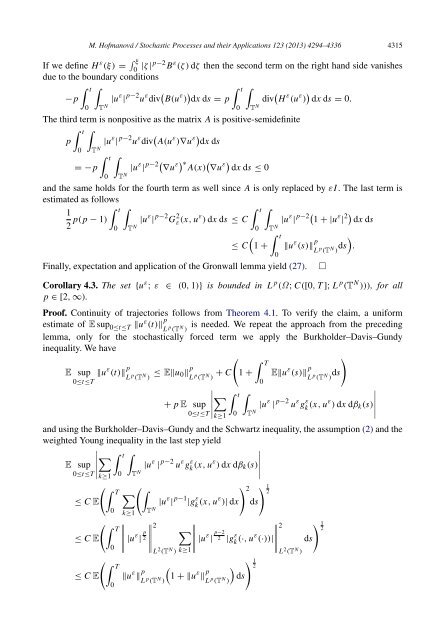
M. Hofmanová / Stochastic Processes and their Applications 123 (2013) 4294–4336 4315
If we define H ε (ξ) = ξ
0 |ζ |p−2 B ε (ζ ) dζ then the second term on the right hand side vanishes
due to the boundary conditions
t
−p |u ε | p−2 u ε div B(u ε ) t
dx ds = p div H ε (u ε ) dx ds = 0.
0 T N 0 T N
The third term is nonpositive as the matrix A is positive-semidefinite
t
p |u ε | p−2 u ε div A(u ε )∇u ε dx ds
0 T N t
= −p |u ε | p−2 ∇u ε ∗
A(x) ∇u
ε dx ds ≤ 0
0 T N
and the same holds for the fourth term as well since A is only replaced by εI . The last term is
estimated as follows
1
t
t
2 p(p − 1) |u ε | p−2 G 2
0 T N ε (x, uε ) dx ds ≤ C |u ε | p−2 1 + |u ε | 2 dx ds
0 T N
t
≤ C 1 + ∥u ε (s)∥
.
p L p (T N ) ds
Finally, expectation and application of the Gronwall lemma yield (27).
Corollary 4.3. The set {u ε ; ε ∈ (0, 1)} is bounded in L p (Ω; C([0, T ]; L p (T N ))), for all
p ∈ [2, ∞).
Proof. Continuity of trajectories follows from Theorem 4.1. To verify the claim, a uniform
estimate of E sup 0≤t≤T ∥u ε (t)∥ p is needed. We repeat the approach from the preceding
L p (T N )
lemma, only for the stochastically forced term we apply the Burkholder–Davis–Gundy
inequality. We have
T
E sup ∥u ε (t)∥ p L
0≤t≤T
p (T N ) ≤ E∥u 0∥
1 p L p (T N ) + C + E∥u ε (s)∥ p L
0
p (T N ) ds
t
+ p E sup
|u ε | p−2 u ε g ε
0 T N k (x, uε ) dx dβ k (s)
0≤t≤T
k≥1
and using the Burkholder–Davis–Gundy and the Schwartz inequality, the assumption (2) and the
weighted Young inequality in the last step yield
t
E sup
|u ε | p−2 u ε g ε
0≤t≤T
k≥1 0 T N k (x, uε ) dx dβ k (s)
T 2 1
2
≤ C E
|u ε | p−1 |g ε
T N k (x, uε )| dx ds
0
k≥1
T
≤ C E
|uε | p 2
0
2
L 2 (T N ) k≥1
|uε | p−2
2 |g
ε
k (·, u ε (·))|
T
≤ C E ∥u ε ∥ p 1 + ∥u ε ∥ p ds
L p (T N )
L p (T N )
0
1
2
0
2
L 2 (T N )
ds
□
1
2